How accurate are the longer-term projections of overall survival for cancer immunotherapy for standard versus more flexible parametric extrapolation methods?

Abstract

Aims

To assess the accuracy of standard parametric survival models, spline models, and mixture cure models (MCMs) fitted to overall survival (OS) data available at the time of submission in the NICE HTA process compared with data subsequently made available.

Methods

Standard parametric distributions, spline models, and MCMs were fitted to OS data presented in single technology appraisals (TAs) for immune-checkpoint inhibitors (ICIs) in cancer. For each TA, the estimated survival from the fitted models was compared with Kaplan–Meier (KM) data that were made available following the HTA submission using differences between point estimates and restricted area under the curve (AUC) at both the midpoint and the end of additional follow-up. Differences in interval AUC values (calculated for each 6-month period) were also assessed.

Results

Standard parametric survival models and spline models were more likely to underestimate longer-term survival, irrespective of the measure used to assess model accuracy. MCMs were more likely to overestimate survival; however, this was improved in some cases by applying an additional hazard of mortality for “statistically cured” patients.

Limitations

The accuracy of the models was assessed based on much shorter OS data than the period for which extrapolation is needed, which may impact conclusions regarding the most accurate models. The most recent TAs for ICIs have not been captured.

Conclusions

There are no definitive findings that unquestionably support the use of one specific extrapolation technique. Rather, each has the potential to provide accurate or inaccurate extrapolation to longer-term data in certain circumstances, but the added flexibility of more complex models can be justified for treatments, like ICIs, that have extended survival for patients across disease areas. The use of mortality adjustments for “statistically cured” patients allows decision-makers to explore more conservative scenarios in the face of high decision uncertainty.

Keywords:

• Immunotherapy
• overall survival
• NICE
• extrapolation
• spline
• mixture cure

JEL Classification Codes:

• C00
• C
• C10
• C1
• C52
• C5

Introduction

Uncertainty around lifetime survival projections based on short-term regulatory trial data are often, if not always, central to decision uncertainty in health technology assessment (HTA). The time between the initiation of new clinical trials, regulatory approval, and subsequent HTA submissions is becoming shorter. To accelerate patient access to innovative medicines identified as having promising benefits, regulatory approvals, and submissions are often based on less mature data and surrogate outcomes or proxies for overall survival (OS) such as progression-free survival¹. However, this leads to a reduction in the extent of long-term clinical trial evidence available to support HTA decisions. As explored by Quinn et al.¹ the issue is further exacerbated for novel treatment options including immune-checkpoint inhibitors (ICIs), a type of immuno-oncology therapy. The mechanism of action for these therapies can lead to a delayed, but lasting, clinical response due to the timing of the immune system response and thus an expectation of marked improvement in clinical outcomes². ICIs have been demonstrated to provide substantial improvements in the long-term survival of patients (the extent of which varies by technology and indication); however, these improvements are often not captured well when the available clinical trial data are less mature^3,4.

Despite these data limitations, long-term estimates of time-to-event outcomes (including OS) are still required to support HTA decisions, given the request of HTA agencies such as the UK National Institute for Health and Care Excellence (NICE) to capture the full benefits (and costs) experienced by patients over their lifetimes⁵. Thus, it is necessary to use methods that allow extrapolation beyond the trial period. The most common methods for extrapolating time-to-event outcomes are standard parametric survival models, the use of which is well documented⁶. However, these models often do not provide sufficient flexibility to reflect the long-term outcomes anticipated for ICIs. This issue has more recently led to the increased consideration in technology appraisals (TAs) of more flexible methods for long-term extrapolation including spline and mixture cure modeling methods and, subsequently, the production of new guidance covering more flexible extrapolation methods⁷. Nevertheless, the most appropriate approaches for accurate long-term extrapolation remain unclear.

Bullement et al.⁸ assessed the accuracy of the extrapolation methods preferred by manufacturers, evidence review groups, and NICE committees for a set of NICE single technology appraisals in oncology when considering subsequent trial data cuts becoming available after the original submission. The review targeted TAs for immunotherapies in cancer indications. Using the TAs identified as part of this prior review and the associated evidence base, we assessed the ability of standard parametric survival models, mixture cure models, and spline models to accurately capture longer-term survival outcomes. For this, we fitted the models to the data used within each HTA submission and compared the generated outcomes with those observed in the longer follow-up survival data. Our aim was to identify any features that may a priori suggest whether some of these methods would be more appropriate for long-term extrapolation under specific circumstances.

Methods

The analyses presented in this paper are based on the systematic search of the NICE website conducted by Bullement et al.⁸ to identify relevant TAs for immunotherapies⁹. This review focused on NICE as the most transparent source of HTA submission evidence and the extensive information that NICE shares publicly. The details of this review have been presented in full previously, but in summary: the search was limited to completed single TAs published between 1 March 2000 and 31 December 2017. The US National Cancer Institute (NCI) definition of an ICI was used to identify all licensed¹⁰ technologies by the European Medicines Agency (EMA) and US Food and Drug Administration (FDA) at the time. This resulted in the following list of cancer ICIs: ipilimumab, pembrolizumab, nivolumab, atezolizumab, durvalumab, and avelumab. To identify available OS data from more recent data cuts than reported in the TA materials, Bullement et al.⁸ conducted a targeted literature search for the relevant pivotal trials associated with each TA. At least one later data cut was required for the inclusion of each TA to allow the accuracy of extrapolations to be assessed; otherwise, the TA was excluded. In addition, if the clinical trial associated with a TA had multiple published data cuts since the TA, the most recent one was used, to provide the most relevant long-term data (as applied by Bullement et al.).

For each TA, OS Kaplan–Meier (KM) plots were digitized for the ICI treatment arms (using digitization software GetData Graph Digitizer)¹¹ to create pseudo-patient-level data using the algorithm of Guyot¹². Pseudo-patient-level OS data were generated from the data cut of the pivotal trial that was presented during the NICE submission, and from the most recent data cut reporting OS KM data. Given changes in follow-up, new events observed and changes in censor times, the end of the earlier KM curve in particular can appear quite different to the shape of the later KM curve. Parametric survival analysis methods that allowed for extrapolation beyond the trial period were then applied to pseudo-patient-level data from the earlier data cut for each TA. Standard parametric models that have been generally recommended until recently were compared with two more flexible analysis methods, which are commonly used in cases where the data and clinical rationale suggest that long-term survival is plausible for a cohort of patients. The three analysis methods included:

• Standard parametric survival models. These models are documented in detail in the NICE Decision Support Unit (DSU) Technical Support Document (TSD) 14 and are among the most common survival models used in NICE submissions⁶. Fitted distributions included the exponential, Weibull, Gompertz, log-logistic, log-normal, and generalized gamma, as well as the generalized F distribution, which allows additional flexibility with the inclusion of a fourth parameter. All standard parametric models were fitted in R using the flexsurv package¹³.

• Spline models¹⁴. These models reflect complex underlying hazards (and thus survival) within the follow-up period through the use of piecewise polynomials, such that the trajectory of the survival curve can change between selected time intervals, determined by the placement of knots. Spline models are considered an extension of a true piecewise model, where the changes between time intervals are smoothed. This flexibility can be used to better reflect changes in hazards that are not always possible to capture within standard parametric distributions¹⁴. However, the use of spline models in economic evaluations is limited, most likely due to the increased difficulty in interpreting these models and, importantly, in providing a clinical justification for their use^15,16. Three spline-based models were considered: the proportional hazards, proportional odds, and the probit models. Each of these models a different transformation of the survival function. Splines were limited to a maximum of three (internal) knots to limit the risk of overfitting, particularly as it is considered unlikely that there is clinical justification to support high numbers of knots, and there seems to be a minimal gain from using more than three internal knots¹⁴. To remove any subjectivity of knot placement, knots were placed at equally spaced quantiles of the log uncensored survival time of the KM curve for each TA. In addition, the placement of knots is not considered a key driver of model fit¹⁴. All splines in our study were fitted in R using the flexsurv package¹³.

• Mixture cure models (MCMs). In general, mixture models are structured to reflect the assumption that there are two (or more) cohorts of patients in the population with differing survival outcomes, and the overall population contains a mixture of these two groups⁷. MCMs are a specific type of mixture model with two groups: one that is considered to reflect those who do not respond well to treatment and have poor outcomes (“uncured”) and one that reflects the outcomes of patients that are anticipated to experience long-term survival (“statistically cured”)^7,17,18. The mixture of patient groups is captured via the estimation of a “cure” fraction, reflecting the proportion of patients who experience long-term survival (“statistically cured”) versus those who do not. The fitted MCM estimates the proportion of patients who do experience long-term survival, as well as a survival model for short-term survivors. For short-term survivors, survival is modeled using the standard parametric survival models listed previously. The survival for long-term survivors is primarily modeled based on age- and gender-matched general population mortality applied from the time of entering into a study and throughout their lifetime¹⁹. In our study, all MCMs were fitted to absolute survival in R using the flexsurvcure package, guided by the approach presented by Grant et al.²⁰, with further details provided in Appendix 3.

Because it was considered optimistic to assume that the survival of long-term survivors follows that of the general population, the application of excess mortality to long-term survivors was also considered when fitting MCM. Published American Joint Committee on Cancer (AJCC) registry data were used to identify long-term, cancer-type-specific survival, where available and appropriate, to estimate the increased risk above general population mortality²¹. In each case, the most appropriate long-term survival curve(s) presented by the AJCC were selected to align most closely with the patient population of the primary trial evidence associated with each TA. Where the trial includes patients at multiple disease stages, the separate survival curves by stage presented by the AJCC were digitized and combined. The increased hazard of mortality for long-term survivors was estimated by comparing age- and gender-matched general population survival estimated for each specific TA with the observed survival of long-term survivors in the indication. US mortality estimates²² were used for general population survival estimates to align with the AJCC data that were collected in the US. The increased hazard for long-term survivors was estimated by first rebasing the estimated general population survival and the registry data survival curve from the approximated point of inflection in the registry data, which suggests only long-term survivors remain alive at that time. Further details on the relevant AJCC data source selected for each TA and the estimated additional hazards of mortality are presented in the Appendix (Table 5).

Following the application of the survival extrapolation approaches to the recreated pseudo-patient-level data from the initial data cut presented in the NICE submission, the Akaike information criterion (AIC) and the Bayesian information criterion (BIC) statistics were calculated. These goodness-of-fit statistics are commonly used in HTA submissions to support the identification of suitable model fits and were recommended for consideration in the NICE DSU TSD 14⁶. However, AIC and BIC only capture the goodness-of-fit to the observed data, and the more recent NICE DSU TSD 21 cautions against the over-interpretation of these values when extrapolating beyond the study follow-up⁷. The new guidance states that model choice should take into consideration the statistical appropriateness and clinical plausibility of survival estimates beyond the observed data for the fitted models. We assessed whether models with good statistical fit to the earlier data cut were aligned with models that provided the most accurate estimates for the longer-term data to understand how reliable goodness-of fit statistics are when used to support model choice. An overall understanding of model fit was explored using plots that compared the models fitted to the initial KM curve and the initial and later KM curves.

Multiple summary measures have been used to further quantify the accuracy of the model projections based on the earlier data cuts when compared with the observed OS KM curves from the later data cuts, including:

• Comparison of the point estimates for survival between the model projection with later OS KM data, summarized based on the difference in the point estimates (dPE; Figure 1).

• Comparison of the estimated restricted area under the curve based on the fitted survival model with the later KM curve, summarized based on the difference between the restricted area under the curve (dRAUC; Figure 1).

Figure 1. Estimation of dPE, dRAUC and dIAUC. Abbreviations. dIAUC, difference between the interval area under the curve; dPE, difference in the point estimates; dRAUC, difference between the restricted area under the curve; FoU, follow-up; KM, Kaplan-Meier.

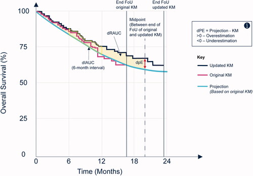
Both quantities were calculated at the midpoint between the end of follow-up of the original data and the end of follow-up of the more mature data. The use of the midpoint follows the rationale presented by Bullement et al.⁸ for a pragmatic trade-off between robustness of the most mature KM data (sufficient patient numbers and increased follow-up time) and the relevance of addressing the research question (i.e. how accurately do the fitted models capture longer-term survival outcomes?). Comparisons of the model projections with the KM curves were also made at the maximum follow-up time of the later KM curve in scenario analyses. This approach used the maximum follow-up information available for each TA and closely aligned with the objectives of this investigation. However, this approach is likely to be more uncertain due to the low numbers at risk generally available at the end of a KM curve.

All differences were calculated based on the estimate from the fitted model minus the estimate from the observed KM curve, such that a positive difference would suggest that the model overestimated the observed KM survival when compared with later data and vice versa (Figure 1). Given the quantity of data, the differences in point estimates and AUC were ranked from the smallest to largest absolute values and the models that were ranked one of the three highest (i.e. the three smallest values) were used to identify the most accurate model types for each TA.

In addition, comparison of the area under the curve with the fitted survival model and the later KM curve for each 6-month interval was explored and summarized as the difference in 6-month interval AUC (dIAUC; Figure 1). Interval estimates are used to explore where deviations between the fitted model and the observed later KM curve occurred (i.e. whether the AUC was consistently over- or underestimated in each 6-month interval of the follow-up period).

Results

The systematic search conducted by Bullement et al.⁸ identified 11 relevant TAs for ICIs (details of this are published elsewhere). Of the 11 TAs identified, 10 were suitable for use in this investigation. One of the TAs (TA400) did not provide an original KM curve, and thus the accuracy of fitted models could not be assessed in this case²³.

The sample sizes, follow-up times for the initial KM curves, and the overall proportion of models that underestimate survival were summarized by TA for the dPE and dRAUC measures at both the midpoint and end of follow-up (Table 1; further detail of dPE and dRAUC values is included in the Appendix [Tables 3 and 4]). Additionally, to reflect model accuracy, the proportion of models within two standard errors of the KM estimate at both the midpoint and end of follow-up were also summarized for dPE.

Table 1. Model fit summary.

Summary		TA319	TA357	TA366	TA384	TA417	TA428	TA447	TA483	TA484	TA490
n		250	180	277	210	410	344	154	135	292	240
Initial follow-up time (months)		47.4	16.6	17.2	16.5	30.5	22.2	18.7	22.7	25.3	16.6
Later follow-up time (months)		72.0	35.1	26.1	27.7	53.8	35.0	33.0	51.8	51.9	24.4
Model fit summary
Survival point estimates (dPE)
Proportion of models that underestimate survival point estimate at midpoint (%)	Std. PSM	100	100	100	57	86	86	50	43	71	29
	Spline	100	100	67	44	100	89	11	0	78	0
	MCM (general population)	100	71	43	0	71	33	0	0	71	0
Proportion of models that underestimate survival point estimate at the end of follow-up (%)	Std. PSM	100	100	100	71	86	71	33	86	100	29
	Spline	100	100	100	67	100	67	0	33	89	0
	MCM (general population)	100	57	43	14	71	17	0	0	100	0
Proportion of models within two standard errors of the Kaplan-Meier estimate at the midpoint (%)	Std. PSM	0	57	71	100	43	71	100	71	57	71
	Spline	67	78	89	100	22	56	100	100	67	78
	MCM (general population)	100	86	100	86	57	57	71	29	71	0
Proportion of models within two standard errors of the Kaplan-Meier estimate at the end of follow-up (%)	Std. PSM	0	71	17	71	43	71	83	71	57	71
	Spline	0	89	56	67	0	89	78	100	56	89
	MCM (general population)	57	71	57	86	43	50	14	29	71	0
Restricted mean survival (dRAUC)
Proportion of models that underestimate restricted mean survival (AUC) at midpoint (%)	Std. PSM	100	100	100	43	100	86	33	0	71	0
	Spline	100	100	100	33	100	89	0	0	78	0
	MCM (general population)	100	100	71	0	100	33	0	0	71	0
Proportion of models that underestimate restricted mean survival (AUC) at the end of follow-up (%)	Std. PSM	100	100	100	57	86	86	33	29	71	0
	Spline	100	100	100	33	100	89	0	0	89	0
	MCM (general population)	100	71	57	0	86	17	0	0	71	0

Abbreviations. AUC, area under the curve; CI, confidence interval; KM, Kaplan–Meier; MCM, mixture cure model; n, number; TA, technology appraisal; Std. PSM, standard parametric survival model.

Notes: Follow-up, survival, and numbers at risk based on digitized data.

The proportion of models that underestimated survival is generally consistent between the two measures used (dPE and dRAUC). There was more variation in the proportion of models that underestimated survival between the two different time points investigated (at the midpoint and at the end of follow-up); however, if the majority of fitted models generally underestimated (or overestimated) at the midpoint, then the same trend was seen at the end of follow-up and vice versa. Standard parametric survival and spline models were more likely to underestimate survival irrespective of the measure used or timepoint, and MCMs were most likely to overestimate survival. In general, smaller trials with shorter follow-up periods tended to be associated with projections that overestimated survival when compared with subsequent data cuts. The proportion of models within two standard errors of the KM estimate generally decreases from the midpoint to the end of follow-up. In general, spline models were most likely to provide accurate estimates, based on estimates within two standard errors of the KM point estimate, and this is consistent at both time points. However, both standard parametric models and MCMs also provide accurate results based on this measure in certain cases and generally, across the TAs, the majority of models provide estimates within two standard errors of the KM point estimate.

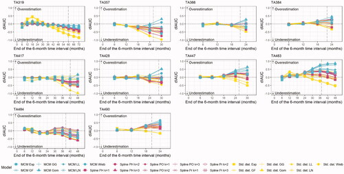
For each 6-month interval, the difference in interval AUC values was calculated (Figure 2). The majority of fitted models led to a consistent or downward trajectory, suggesting a trend towards underestimating survival. There was a higher likelihood of model underestimation for those TAs with longer follow-up and larger patient numbers (TA319, TA417, and TA484) and a higher likelihood of overestimation for those TAs with shorter follow-up and lower patient numbers (TA447, TA483, and TA490). A majority of models underestimated survival both at the midpoint and end of follow-up; in total, seven of the TAs for standard parametric survival models, six of the TAs for splines, and four of the TAs for MCMs. Standard parametric survival models were most likely to provide extreme underestimations over time, while MCMs were most likely to lead to extreme overestimations. The MCMs that resulted in extreme overestimations were often also shown to provide poor accuracy based on dPE. For example, the MCM where a Gompertz distribution was used to model the survival for short-term survivors was consistently shown to lead to one of the most extreme overestimation trajectories (where the model increasingly overestimated survival over time). This aligned with the findings from Cooper et al.²⁴ where the MCM Gompertz was only shown to provide one of the three most accurate models for one TA, based on dPE at the midpoint of additional follow-up.

Figure 2. Six-month interval restricted mean survival (dIAUC) for each TA. Abbreviations. dIAUC, difference between the interval area under the curve; Exp, exponential; GF, Generalized F; GG, generalized gamma; Gom, Gompertz; LL, log-logistic; LN, log-normal; MCM, mixture cure model; PH, proportional hazards; PO, proportional odds; Pr, probit; Std., standard; PSM, parametric survival model; TA, technology appraisal; Weib, Weibull.

Expanding on the results presented previously by Cooper et al.,²⁴ spline models were least likely to provide an “extreme” over- or underestimate and led to dPEs that ranked within the lowest three dPE values in seven of the 10 included TAs, both at the midpoint and at the end of the additional follow-up. Standard parametric models were most likely to underestimate survival and led to the largest underestimates in nine of the 10 TAs considered. However, standard models also led to dPEs that ranked within the lowest three dPE values in four of the 10 TAs at the midpoint, increasing to seven at the end of the later KM follow-up. MCMs provided one or more of the three lowest dPEs for seven TAs calculated at the midpoint of the additional KM follow-up and for six TAs when the dPE was calculated at the end of the additional follow-up. However, MCMs were the most consistent model type to overestimate survival, and it was noted that this generally occurred for the trials with the lowest sample size and more immature follow-up for the initial data cut.

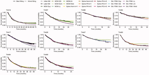
The three best- and worst-fitting models based on the dPE at the midpoint of the additional follow-up are explored further by TA in Figure 3. In five of the 10 TAs the three worst-fitting models underestimate survival and in three cases they overestimate survival. The MCM models are heavily influenced by any demonstration of a “plateau” in the initial KM, which influences the later trajectory for these models. Where evidence for the plateau is weakest (i.e. where the survival probability is still high when follow-up time is short or where the numbers at risk are consistently low towards the end of the KM), this leads to cases where MCMs provide the largest overestimates of longer-term survival. Similarly, in these cases it is more likely that the standard parametric models will lead to the greatest underestimates of longer-term survival. The best-fitting spline models are less likely to be influenced by the end of the initial KM than the MCMs. As already highlighted by Cooper et al.,²⁴ generally, the lowest AICs (indicating the best-fitting model) did not consistently align with the lowest dPEs in any of the TAs.

Figure 3. KM and best and worst fitting models overlaid for each TA. Abbreviations. Exp, exponential; GF, generalized F; GG, generalized gamma; Gom, Gompertz; KM, Kaplan-Meier; LL, log-logistic; LN, log-normal; MCM, mixture cure model; PH, proportional hazards; PO, proportional odds; Pr, probit; Std., standard; PSM, parametric survival model; TA, technology appraisal; Weib, Weibull.

Assessing model fit based on the difference in restricted AUC shows some consistency with the results based on dPE. MCMs were most likely to provide at least one of the three most accurate estimates (seven TAs at the midpoint and six at the end of the additional follow-up), followed by the standard parametric survival models (six and five at the midpoint and end of additional follow-up, respectively). Splines provided fewer of the most accurate models based on dRAUC values rather than dPE, although, unlike MCMs and standard parametric models, the accuracy of these models generally improved by the end of follow-up (three at the midpoint and six at the end of follow-up). This aligns with the finding that spline models were least likely to provide an “extreme” over- or underestimate towards the end of the follow-up and may be due to lack of prespecified performance expectation unlike MCMs.

In analyses presented previously by Cooper et al.²⁴, the accuracy of each fitted model was assessed based on dPE values at the primary midpoint timepoint. The proportion of models in our study that underestimated survival is presented in Table 1, indicating that MCMs were more likely to overestimate survival than both splines and standard parametric survival models. To reflect the possibility that, though being long-term survivors, these patients may still be at an increased mortality risk compared with the general population, an excess hazard for these patients was applied.

The estimated additional hazards of mortality applied to the MCMs for each TA are presented in the Appendix (Table 5). The estimated hazards are notably high in some cases, which could suggest that the point of inflexion is too soon or that the source of long-term survival may not be appropriate. However, these estimates can provide an example of a possible extreme case in each scenario.

The application of an additional hazard of mortality reduced the proportion of MCMs that overestimated survival (see Table 2). In addition, despite the high additional mortality estimated in some cases, the application of an additional hazard for the proportion of patients estimated to be long-term survivors provides a similar or improved dPE (smaller absolute dPE at the midpoint) for at least one of the seven MCMs in all except one TA. In cases where the dPE at the midpoint is reduced following the application of additional hazard (highlighted in green in Table 2), the average improvement (3.75%) is greater than cases where the dPE at the midpoint increased, with an average worsening (red cells) in the dPE of 2.59%. This suggests that the application of an additional hazard for mortality can improve the estimate of the longer-term survival. Importantly, adjustment for additional mortality reduced model accuracy for some TAs with the largest sample sizes and follow-up, with the greatest benefits in accuracy shown for trials with the lowest sample sizes and shortest follow-up.

Table 2. Comparison of MCM dPEs at the midpoint when adjusted for general population mortality or with the general population subject to additional excess mortality.

	TA319		TA357		TA366		TA384		TA417		TA428		TA447		TA483		TA484		TA490
N	250		180		277		210		410		344		154		135		292		240
Initial follow-up time (months)	47.4		16.6		17.2		16.5		30.5		22.2		18.7		22.7		25.3		16.6
	No additional hazard	Additional hazard	No additional hazard	Additional hazard	No additional hazard	Additional hazard	No additional hazard	Additional hazard	No additional hazard	Additional hazard	No additional hazard	Additional hazard	No additional hazard	Additional hazard	No additional hazard	Additional hazard	No additional hazard	Additional hazard	No additional hazard	Additional hazard
Exponential	−3.3	−6.0	−8.2	−8.2	−4.2	−4.2	0.5	−3.1	−2.0	−2.1	−2.4	−4.8	3.9	−7.1	5.8	0.9	−5.8	−6.5	6.5	4.9
Generalized F	−3.9	−5.8	−4.3	−4.3	3.2	−0.7	3.6	3.6	−7.4	−9.8	NA	NA	7.3	−3.9	8.1	5.2	1.2	1.2	7.0	7.0
Generalized Gamma	−3.9	−5.8	−4.2	−4.3	4.9	0.7	3.6	3.6	−7.0	−13.6	10.3	1.2	9.4	−4.3	12.0	4.9	1.2	1.2	7.0	6.9
Gompertz	−2.0	−5.1	5.5	2.5	5.2	1.0	7.9	3.1	0.2	−14.5	10.0	1.0	10.7	−3.3	13.8	6.2	−5.1	−5.1	9.4	7.1
Log-logistic	−3.4	−5.3	−1.7	−2.6	−2.3	−4.7	3.5	−0.4	−2.5	−2.9	−0.2	−1.1	4.7	−4.4	8.5	3.6	−0.6	−0.8	8.9	7.5
Log-normal	−3.9	−5.8	−2.5	−2.5	−3.1	−3.1	2.8	−0.8	1.2	1.2	1.2	1.2	2.9	2.8	5.0	2.0	−0.8	−0.8	7.1	6.2
Weibull	−1.3	−4.6	2.3	−0.3	0.5	−3.3	5.7	1.1	−8.1	−11.1	5.2	−2.3	7.5	−5.4	13.1	5.7	−3.5	−5.9	10.6	8.2
Proportion of models that underestimate survival point estimate at midpoint	100%	100%	71%	86%	43%	71%	0%	43%	71%	86%	33%	50%	0%	86%	0%	0%	71%	71%	0%	0%

Abbreviations. dPE, difference in point estimate; MCM, mixture cure model.

Notes. Red cells indicate a larger absolute dPE with additional hazard (reduced accuracy); green cells indicate a reduced dPE with additional hazard (improved accuracy).

Following this adjustment, the influence of any potential “plateau” or low number of patients at risk in the KM curve is also reduced, as the additional mortality hazard is applied to the proportion of patients who were estimated to be statistically cured. For example, the MCM Gompertz curve for TA447 (the TA with the second smallest patient population) presented in Table 2 overestimates survival at the midpoint by 7.90%; this is reduced to 3.10%, when the additional hazard for mortality is applied. Similarly, for TA483 (the TA with the smallest patient population), the overestimation of survival at the midpoint for the Weibull, Gompertz, and generalized gamma curves is reduced by 55.10–59.20% for the models with additional hazard compared with those without. Conversely, for the most conservative models, such as the MCM exponential, the application of excess mortality is more likely to reduce the accuracy of the fitted model based on differences in point estimates.

Discussion

The development of novel immunotherapies in oncology has further increased the challenges surrounding the estimation of long-term survival due to the use of survival data with limited follow-up. Two of the three key challenges identified by Quinn et al.¹ for assessing the long-term benefits of immunotherapies are the differing mechanism of action from which follows a lack of agreement on the ideal methods for extrapolating survival for these treatments. These challenges have led to increased consideration of more flexible methods for extrapolation and new guidance for these methods⁷. Our analyses provide additional insight into the accuracy of standard parametric models compared with two more flexible methods, splines and MCMs, which are being more frequently considered to support HTA decisions to account for the impact of the differing mechanism of action for ICIs.

For 10 TAs identified in a previously conducted systematic search, we compared the accuracy of the three types of survival models⁸. These were fitted to the data cut used to support the NICE HTA decision and compared with survival data that were later made available. Along with visual inspection of the curves, three different measures of accuracy were considered: dPEs for survival and dRAUCs (both calculated at the midpoint of the additional follow-up and the end of the additional follow-up), as well as differences in the interval AUC, calculated for each 6-month interval.

Generally, each of the measures favors the same model type/types; that is, the model types that are most accurate based on dPEs were generally the most accurate models based on other measures (AUC and interval AUC values). However, there was some variation in the exact models in each overall model type that were most accurate. As presented previously²⁴, AIC did not align well with the models that provided the closest point estimates based on dPE and this also holds for restricted AUC, suggesting that it is likely inappropriate to use measures of statistical fit, like AIC and BIC, as a basis for choosing models that represent clinically plausible projections in the longer-term.

Based on dPE and dRAUC at the midpoint and the end of additional follow-up, standard distribution models were most likely to underestimate longer-term survival. The MCMs generally produced the largest proportion of models that overestimated survival and standard parametric distributions generally produced the largest proportion of models that underestimated survival. This latter observation aligns with that of Ouwens et al.²⁵ who also found that standard parametric models generally underestimated longer-term OS compared with later data.

Spline models and MCMs were both more likely than standard parametric survival models to provide one of the most accurate models based on dPE (within the three smallest dPE values). This was also the case for MCMs based on dRAUC. The number of cases where spline models or standard parametric survival models led to the most accurate survival estimates (within the three smallest dPEs) was consistent or increased when estimating the dPE at the end of follow-up, compared with the midpoint. For MCMs, this number decreased by one TA when estimating at the end of follow-up. For dRAUC, both standard parametric survival models and MCMs led to fewer of the most accurate models at the end of follow-up compared with the midpoint of initial follow-up, whereas this number increased for spline models. The accuracy of spline models based on dPE and dRAUC (where accuracy in the latter increased from the midpoint to end of follow-up) aligns with the findings of Gray et al., who found that spline models perform well at projecting OS fitted to registry cohorts with artificially right-censored follow-up time²⁶.

The 6-month interval AUCs were explored to understand how the accuracy of model extrapolations changed over time. Generally, the tendency for standard models to produce the greatest underestimations and for MCMs to produce the greatest overestimations became more pronounced over time. Importantly, the poorest trajectories (largest overestimations or underestimations) for differences in 6-month interval AUCs did not generally align with the specific MCMs and standard parametric survival models that provide the most accurate estimates.

As stated previously by Cooper et al.²⁴, it is difficult to conclude which models will generally under- or overestimate survival. However, the authors concluded there was a higher likelihood of model overestimation with lowest sample sizes and more immature follow-up for the initial data cut, and this was consistent across dPE and dRAUC both at the midpoint and end of additional follow-up. In addition, for TAs with a short initial follow-up, the pattern of under- or overestimation was unclear. However, in cases where sample sizes, initial follow-up time, and the numbers at risk towards the end of initial follow-up were lowest – particularly when the KM curve shows a “plateau” based on these low numbers at risk – we observed that models were more likely to overestimate. Specifically, the trajectories of the MCMs were likely to be most sensitive to these unsupported “plateaus”.

The application of an additional hazard of mortality for the proportion of patients who were estimated to be statistically “cured” for the MCM extrapolations reduced the proportion of MCMs that overestimated longer-term survival and lead to greater improvement in accuracy on average. However, the TAs with the shortest follow-up and smallest sample sizes tended to benefit most from the application of additional hazard, whereas accuracy for survival estimates for TAs with the longest follow-up and largest sample sizes decreased in some cases. This observation is not unexpected given that that these trials are likely to better capture excess mortality in the observed trial outcomes. The consideration of external data for MCMs (and other more flexible models) is anticipated to be an essential requirement for the purposes of NICE HTA submissions based on the guidance presented in NICE TSD 21^7,27. Given the possible impact on survival outcomes following the incorporation of external data, this study highlights the need to carefully consider and justify the selected source of the additional hazard of mortality (or other external data source), as well as the clinical plausibility of the selected models across the whole time period required for extrapolation.

Our assessment of model accuracy using a comparison of point estimates, AUC values, and interval AUC values, as well as a visual assessment of the curves, suggests that spline models and MCMs have the potential to provide accurate estimates of longer-term survival. Ouwens et al.²⁵ came to a similar conclusion for MCMs when investigating the accuracy of extrapolating OS for patients treated for non-small-cell lung cancer with durvalumab. Our assessment also suggests that all three model types can be appropriate options to estimate survival in certain TAs, again similar to Ouwens et al., who found it difficult to identify consistent uses of models to extrapolate survival data. Similarly, Roth et al.²⁸ found strong similarities in survival estimates between MCM and standard parametric survival extrapolations. The authors proposed that this was likely due to the lack of data maturity or the small proportion of long-term survivors and noted that in this situation, the use of MCMs may not be warranted. The clinical plausibility and rationale of the underlying assumptions of the applied methodology should, therefore, be carefully assessed when considering their use, particularly in the case of the more flexible spline models or MCMs.

We acknowledge that the presented analyses have some limitations. This research has been conducted based on a systematic search of the NICE website and the targeted literature search for later data cuts that were performed and presented by Bullement et al.⁸ These were not updated for the purpose of these analyses. We acknowledge that a substantial number of additional TAs for ICIs are now available. The consideration of more recent ICI trial data with multiple data cuts (and of any more recent data cuts for the currently identified TAs) would allow the general trends identified in these analyses to be assessed and would be a valuable addition to this work.

We focused our comparison of model accuracy on standard parametric survival models, spline models, and MCMs; however, NICE TSD 21 guidance, published shortly after this work was conducted, includes these flexible model types as well as several other methods that have not been considered here. In addition, the assessment of model accuracy remains limited by the extent of additional follow-up provided for each TA, which is still considerably shorter than the length of the extrapolation required for HTA decision-making. For the time horizon estimates that are required to support economic model development, the clinical plausibility of extrapolations remains an essential consideration for any fitted model. Clinical plausibility and the use of external data for the purpose of validation or for incorporation into the survival extrapolation is discussed in detail in the recently published NICE DSU TSD 21⁷. This study focuses on spline and MCM methods, which both feature in the NICE guidance. However, the authors acknowledge that there are a range of other extrapolation methods as well as methods for incorporating external data that have not been considered here. In particular, spline models (or flexible parametric models) that incorporate external data as part of the model fitting have been demonstrated to provide the potential for accurate long-term extrapolations⁷. In addition, as described above, the assessment of model accuracy is based on three different measures: dPEs, dRAUCs and differences in the interval AUC, calculated for each 6-month interval along with visual inspection of the curves. Of note for dRAUC in particular, this measure captures the overall difference in RAUC, and therefore may not capture instances where the over- and underestimates across the relevant time period cancel out, however this measure is used in combination with other measures of accuracy where this detail is better captured. The authors recognize that there are likely many alternative measures (such as differences in mean OS, or the proportion of time where models more closely reflect the KM curve) that could also be considered as part of future research.

The general population adjustment (with or without excess mortality) applied for the long-term surviving cohort of the MCMs for the purpose of extrapolation was conducted after the model was fitted. The incorporation of external data into the model fitting process may influence the estimated cure fraction and subsequent model parameters of the short-term survivor cohort and therefore may affect these conclusions. However, our analyses demonstrate that the use of MCMs can be a viable option in some cases and has the ability to be more flexible for cost-effectiveness model requirements (such as to explore the impact of different mortality adjustments).

Finally, the estimation of excess mortality for the MCMs was based on a review of the AJCC registry information; this information was selected based on the most comparable disease indication and stage of disease to the population in each TA, but this was limited to what was available in the AJCC. In particular, there were several specific features for the populations in the TAs that could not be captured based on the data in the AJCC registry, including any differences between long-term outcomes between treated and untreated populations, the inclusion/exclusion of patients with mutations, brain metastases, and squamous/non-squamous disease.

Conclusions

• The maturity of the initial follow-up data alone did not provide a clear indication of whether models were likely to under- or overestimate survival beyond the observed period. However, the potential to overpredict survival beyond the end of follow-up where data are most immature should be carefully considered.

• Across the range of measures used to assess the accuracy of model fit, the more flexible spline and MCM models were generally demonstrated to have the potential to accurately reflect longer-term survival, but all models were shown to provide viable options for longer-term estimation of survival in certain cases. However, over- and under-estimations were still observed in a substantive number of cases with all approaches and so the rationale behind the use of any model should be carefully justified based on clinical plausibility and the relevant trial data.

• The addition of excess mortality to the general population for MCMs may be a viable clinically plausible way to reduce the likelihood of MCMs (and other models) overestimating longer-term survival; however, identification of the source of excess hazard is subjective and should be carefully justified. The benefits in accuracy from this process are likely to be greatest in scenarios where trial follow-up is shortest and sample sizes smallest, and these aspects are useful to consider when making decisions on how best to estimate long-term outcomes.

• Extrapolation to support HTA decision-making often requires lifetime projection, which is much longer than the additional follow-up available for these analyses. The clinical plausibility of the extrapolations across the whole time period for extrapolation should be carefully considered and justified when selecting models, particularly in cases where most data are immature.

Transparency

Declaration of funding

This study and manuscript were supported by funding from Merck Sharp & Dohme Corp., a subsidiary of Merck & Co., Inc., Kenilworth, NJ, USA, and Merck, Sharp & Dohme Limited, Hoddesdon, UK.

Declaration of financial/other interests

MC, SS, and TW are employees of BresMed. BresMed received consultancy fees from Merck Sharp & Dohme Ltd for the development of this research and the writing of this manuscript. The authors did not receive direct payment as a result of this work outside of their normal salary payments. RAI is an employee of Merck Canada Inc., a subsidiary of Merck & Co., Inc., Kenilworth, NJ, USA.

Peer reviewers on this manuscript have no relevant financial or other relationships to disclose.

Previous presentations

Earlier analyses of this study were presented as a poster (PCN293) at Virtual ISPOR US 2020.

Acknowledgements

We thank Tara Harding and Ash Bullement for their input during the development of this research, Will Sullivan for his support and input during the development of this manuscript, and Jake Horgan for his editorial support during the development of this manuscript.

Appendix 1.

dPE and dRAUC values at both the midpoint and end of follow-up for the three most accurate fitting models

Table 3. dPE and dRAUC values at both the midpoint and end of follow-up for the top three most accurate fitting models.

Top three most accurate models	dPE midpoint: model (value)	dPE end of follow-up: model (value)	dRAUC midpoint: model (value)	dRAUC end of follow-up: model (value)
TA319
1	MCM Weib	MCM Weib	MCM Weib	MCM Weib
	(0.01)	(0.02)	(−0.29)	(−0.47)
2	MCM Gom	MCM Gom	MCM Gom	MCM Gom
	(0.02)	(0.02)	(−0.39)	(−0.66)
3	MCM Exp	MCM Exp	Std. PSM Gom	MCM Exp
	(0.03)	(0.04)	(−0.47)	(−0.97)
TA357
1	MCM LL	MCM LN	MCM Gom	MCM Weib
	(0.02)	(0.01)	(−0.29)	(0.13)
2	MCM Weib	Std. PSM LN	MCM Weib	MCM Gom
	(−0.02)	(0.01)	(−0.37)	(0.58)
3	MCM LN	Spline PO k = 1	MCM LN	MCM LL
	(0.02)	(0.01)	(−0.49)	(−0.60)
TA366
1	Spline PH k = 3	Spline PO k = 3	MCM GF	Spline PO k = 3
	(0.00)	(0.01)	(−0.01)	(−0.01)
2	Spline Pr k = 3	Spline Pr k = 3	MCM GG	Spline Pr k = 3
	(0.00)	(0.01)	(0.02)	(−0.02)
3	MCM Weib	MCM Weib	MCM Gom	Spline PH k = 3
	(0.00)	(−0.01)	(0.03)	(−0.03)
TA384
1	Spline PH k = 1	MCM Exp	Std. PSM LN	Std. PSM LN
	(0.00)	(0.00)	(0.05)	(−0.07)
2	MCM Exp	Std. PSM Gom	MCM Exp	Spline PH k = 1
	(0.00)	(0.01)	(0.07)	(0.10)
3	Spline PO k = 1	Spline Pr k = 1	Std. PSM LL	MCM Exp
	(−0.01)	(0.01)	(−0.08)	(0.11)
TA417
1	MCM Gom	Std. PSM LN	Std. PSM LN	MCM Gom
	(0.00)	(0.00)	(−0.09)	(−0.14)
2	MCM LN	MCM LN	MCM LN	Std. PSM LN
	(−0.01)	(0.00)	(−0.09)	(0.14)
3	Std. PSM LN	MCM LL	Std. PSM LL	MCM LN
	(−0.01)	(0.04)	(−0.43)	(0.15)
TA428
1	MCM LL	Spline PO k = 1	MCM LL	Spline PO k = 3
	(0.00)	(0.00)	(−0.01)	(−0.02)
2	Spline PH k = 3	Std. PSM LL	Spline PH k = 3	MCM LL
	(0.00)	(0.00)	(0.02)	(0.03)
3	Spline PO k = 3	Spline Pr k = 3	Spline PO k = 3	Spline PH k = 3
	(0.00)	(−0.01)	(−0.06)	(0.07)
TA447
1	Spline PH k = 1	Std. PSM Weib	Std. PSM Weib	Std. PSM LL
	(0.01)	(0.01)	(−0.06)	(0.16)
2	Std. PSM GG	Std. PSM Exp	Std. PSM LL	Spline PH k = 1
	(−0.01)	(0.04)	(0.10)	(0.22)
3	Std. PSM LL	Spline PH k = 1	Spline PH k = 1	Std. PSM Weib
	(0.01)	(−0.04)	(0.17)	(−0.31)
TA483
1	Spline Pr k = 1	Spline PO k = 1	Std. PSM Weib	Std. PSM LL
	(0.00)	(0.00)	(0.11)	(0.18)
2	Spline PH k = 1	Std. PSM Gom	Std. PSM Exp	Spline Pr k = 1
	(0.00)	(0.01)	(0.17)	(0.55)
3	Std. dist. LL	Spline PH k = 2	Std. PSM LL	Spline PH k = 1
	(0.00)	(−0.01)	(0.46)	(0.59)
TA484
1	Spline Pr k = 1	Std. PSM GG	Spline Pr k = 1	Spline Pr k = 1
	(−0.01)	(0.00)	(0.07)	(0.00)
2	MCM LL	Std. PSM GF	MCM LL	MCM GG
	(0.01)	(0.00)	(−0.07)	(0.17)
3	MCM LN	MCM GF	MCM LN	MCM GF
	(0.01)	(0.00)	(−0.08)	(0.17)
TA490
1	Std. PSM Weib	Spline PH k = 3	Std. PSM Exp	Std. PSM Exp
	(0.02)	(0.00)	(0.12)	(0.02)
2	Spline PH k = 3	Spline PH k = 2	Std. PSM Weib	Std. PSM Weib
	(−0.02)	(−0.01)	(0.13)	(0.03)
3	Std. PSM Exp	Spline Pr k = 3	Std. PSM LL	Std. PSM LL
	(0.02)	(−0.02)	(0.28)	(0.43)

Abbreviations. dPE, difference in the point estimates; dRAUC, difference between the restricted area under the curve; Exp, exponential; GF, generalized F; GG, generalized gamma; Gom, Gompertz; LL, log-logistic; LN, log-normal; MCM, mixture cure model; PH, proportional hazards; PO, proportional odds; Pr, probit; Std., standard; PSM, parametric survival model; Weib, Weibull.

Appendix 2.

dPE and dRAUC values at both the midpoint and end of follow-up for the three least accurate fitting models

Table 4. dPE and dRAUC values at both the midpoint and end of follow-up for the top three least accurate fitting models.

Top three least accurate models	dPE midpoint: model (value)	dPE end of follow-up: model (value)	dRAUC midpoint: model (value)	dRAUC end of follow-up: model (value)
TA319
1	Std. PSM Exp	Std. PSM Exp	Std. PSM LL	Std. PSM Exp
	(0.12)	(0.15)	(−1.28)	(−2.60)
2	Std. PSM Weib	Std. PSM Weib	Std. PSM Exp	Std. PSM Weib
	(0.12)	(0.14)	(−0.92)	(−2.49)
3	Std. PSM LL	Std. PSM LN	Std. PSM Weib	Std. PSM LL
	(0.08)	(0.10)	(−0.88)	(−2.40)
TA357
1	Std. PSM Gom	Std. PSM Gom	Std. PSM Weib	Std. PSM Gom
	(0.15)	(0.16)	(−1.49)	(−2.99)
2	Std. PSM Weib	Std. PSM Weib	Std. PSM Gom	Std. PSM Weib
	(0.14)	(0.15)	(−1.46)	(−2.92)
3	Spline PH k = 2	MCM Gom	Spline PH k = 2	Spline PH k = 2
	(0.11)	(−0.14)	(−1.15)	(−2.25)
TA366
1	Std. PSM Gom	Std. PSM Gom	Std. PSM Gom	Std. PSM Gom
	(0.09)	(0.16)	(−0.37)	(−0.89)
2	Std. PSM Weib	Std. PSM Weib	Std. PSM Weib	Std. PSM Weib
	(0.09)	(0.15)	(−0.32)	(−0.81)
3	Spline PH k = 1	Spline PH k = 1	Std. PSM Exp	Spline PH k = 1
	(0.06)	(0.11)	(−0.31)	(−0.63)
TA384
1	MCM Gom	Std. PSM Exp	MCM Gom	MCM Gom
	(−0.08)	(0.12)	(0.4)	(0.95)
2	Std. PSM Exp	Std. PSM Weib	Spline PH k = 3	MCM Weib
	(0.07)	(0.11)	(0.37)	(0.71)
3	Std. PSM Weib	MCM Gom	Spline PO k = 3	Spline PH k = 3
	(0.06)	(−0.10)	(0.37)	(0.66)
TA417
1	Std. PSM Gom	Std. PSM Gom	Std.PSM Gom	Std. PSM Gom
	(0.16)	(0.22)	(−1.61)	(−3.68)
2	Std. PSM Weib	Std. PSM Weib	Std. PSM Weib	Std. PSM Weib
	(0.10)	(0.13)	(−1.07)	(−2.29)
3	Spline PH k = 1	Spline PH k = 1	Spline PH k = 1	Spline PH k = 1
	(0.09)	(0.13)	(−1.06)	(−2.25)
TA428
1	MCM GG	MCM GG	Std. PSM Weib	MCM GG
	(−0.10)	(−0.16)	(−0.54)	(1.27)
2	MCM Gom	MCM Gom	Spline PO k = 2	MCM Gom
	(−0.10)	(−0.16)	(−0.5)	(1.23)
3	Std. PSM Weib	MCM Weib	Spline Pr k = 2	Std. PSM Weib
	(0.08)	(−0.10)	(−0.45)	(−1.07)
TA447
1	MCM Gom	MCM Gom	MCM Gom	MCM Gom
	(−0.11)	(−0.22)	(0.7)	(1.81)
2	MCM GG	MCM GG	MCM GG	MCM GG
	(−0.09)	(−0.20)	(0.63)	(1.62)
3	MCM Weib	MCM Weib	MCM GF	MCM Weib
	(−0.08)	(−0.18)	(0.56)	(1.36)
TA483
1	MCM Gom	MCM Gom	MCM Gom	MCM Gom
	(−0.14)	(−0.16)	(1.92)	(4.07)
2	MCM Weib	MCM Weib	MCM Weib	MCM Weib
	(−0.13)	(−0.15)	(1.89)	(3.93)
3	MCM GG	MCM GG	MCM GG	MCM GG
	(−0.12)	(−0.14)	(1.77)	(3.64)
TA484
1	Spline PH k = 3	Spline PH k = 3	Spline PH k = 3	Spline PH k = 3
	(0.08)	(0.10)	(−0.77)	(−2.04)
2	Spline PH k = 2	Spline PH k = 2	Spline PH k = 2	Spline PH k = 2
	(0.08)	(0.10)	(−0.76)	(−2.03)
3	Std. PSM Weib	Std. PSM Weib	Std. PSM Weib	Std. PSM Weib
	(0.08)	(0.10)	(−0.65)	(−1.86)
TA490
1	MCM Weib	MCM Weib	MCM Weib	MCM Weib
	(−0.11)	(−0.12)	(0.64)	(1.12)
2	MCM Gom	MCM Gom	Spline PO k = 1	MCM Gom
	(−0.09)	(−0.11)	(0.61)	(1.00)
3	MCM LL	MCM LL	MCM LL	MCM LL
	(−0.09)	(−0.09)	(0.59)	(0.97)

Abbreviations. dPE, difference in the point estimates; dRAUC, difference between the restricted area under the curve; Exp, exponential; GF, generalized F; GG, generalized gamma; Gom, Gompertz; LL, log-logistic; LN, log-normal; MCM, mixture cure model; PH, proportional hazards; PO, proportional odds; Pr, probit; Std., standard; PSM, parametric survival model; Weib, Weibull.

Appendix 3.

Mixture cure models and additional mortality

The overall survival for the “mixture” of short- and long-term survivors was calculated using the survival for the constituent parts in combination with the proportion of patients, estimated by the “cure” fraction, that follow each survival trajectory²⁰. The estimated proportion of long-term survivors (the “cure” fraction) was assumed to follow the derived general population mortality, and the estimated proportion of short-term survivors (1 – the “cure” fraction) followed survival estimated by the fitted parametric survival model. When incorporating additional mortality for long-term survivors, the estimated additional hazard was applied to the general population survival before following the same approach set out above.

Table 5 presents details on the data used to derive additional hazards of mortality for long-term survivors when fitting MCMs. The additional hazard for long-term survivors was estimated by comparing AJCC registry data for specific tumor types to the age- and gender-matched general population survival estimates from each TA by first generating two sets of pseudo patient-level data for each TA: one from digitized AJCC data, per tumor type considered in each TA, described in Table 5 and the other from the age- and gender-matched general population survival specific to each TA.

To estimate the excess mortality for long-term survivors, the survival from AJCC targeted to the relevant tumor type was compared to the general population survival after the time where it was believed that the patients remaining alive in the AJCC population were considered long-term survivors, that is, when survival for these patients appeared to level out after a certain length of time and reached an inflection point. This point of inflection was approximated by visual inspection of the AJCC curves to identify the timepoint at which the survival curve began to flatten. Simple hazard plots were also inspected to support the selection of the point of inflection. Once an approximate inflection point was determined (with the selected excess mortality source data timepoint shown in Table 5), both sets of pseudo patient-level data were rebased to exclude data with any time value occurring before this. Cox proportional hazards models were then fitted to the rebased pseudo patient-level data, resulting in estimated excess hazard ratios for long-term survivors compared to the age- and gender-matched general population survival from each TA, that could then be applied to long-term survivors in the MCMs.

Table 5. Additional mortality for mixture cure models.

TA	N	Excess mortality source data and further detail	Excess mortality source data timepoint	Estimated hazard
TA319	250	AJCC, Melanoma of the skin – data digitized and combined from 3 separate metastatic populations:	3 years	7.67 (4.79–12.28)
TA357	180			5.41 (3.38–8.66)
TA366	277			5.13 (3.53–7.47)
TA384	210	M1a: metastases to skin, subcutaneous, or distant lymph nodes		4.88 (3.21–7.41)
		M1b: metastases to lung
		M1c: metastases to all other visceral sites or distant metastases to any site combined with elevated LDH
TA417	410	AJCC, data digitized for Stage IV kidney cancer	3 years	16.98 (9.31–30.98)
TA428	344	AJCC, data digitized for Stage IV NSCLC	4 years	14.16 (9.98–20.07)
TA447	154			12.06 (7.7–18.9)
TA483	135	AJCC, data digitized and combined from Stage IIIb and IV NSCLC		10.84 (6.67–17.64)
TA484	292			12.88 (8.90–18.64)
TA490	240	AJCC, data digitized and combined from three separate head and neck cancer populations:	3 years	8.71 (3.91–19.41)
		Larynx:
		data combined from Stage III and IV
		Oral:
		data combined from Stage II and IV
		Pharynx:
		data combined from Stage II and IV

Abbreviations. AJCC, American Joint Committee on Cancer; LDH, lactate dehydrogenase; NSCLC, non-small cell lung cancer; TA, technology appraisal.

Note: Estimated hazards presented in Table 4 were generated using Cox proportional hazard modeling. The estimated hazard is the hazard associated with the AJCC population compared to US general mortality based on US life tables from the Centers for Disease Control and Prevention. Excess mortality data were used from the timepoint when survival curves began to level off, which was 3 years for the populations with melanoma, kidney, and head and neck cancers and 4 years for the population with NSCLC.

References

- Quinn C, Garrison LP, Pownell AK, et al. Current challenges for assessing the long-term clinical benefit of cancer immunotherapy: a multi-stakeholder perspective. J Immunother. 2020;8(2):e000648.
- Latimer N, editor. Estimating survival benefit for health technology assessment. New challenges presented by immuno-oncology treatments? Basel:BBS/PSI 1-Day Scientific Meeting; 2017. Available from: http://bbs.ceb-institute.org/wp-content/uploads/2017/06/Session4_NicholasLatimer.pdf
- Dine J, Gordon R, Shames Y, et al. Immune checkpoint inhibitors: an innovation in immunotherapy for the treatment and management of patients with cancer. Asia Pac J Oncol Nurs. 2017;4(2):127–135.
- Schadendorf D, Hodi FS, Robert C, et al. Pooled analysis of long-term survival data from phase II and phase III trials of ipilimumab in unresectable or metastatic melanoma. J Clin Oncol. 2015;33(17):1889–1894.
- National Institute for Health and Care Excellence. Guide to the methods of technology appraisal. 5 The reference case 2013. [02 May 2021]. Available from: https://www.nice.org.uk/process/pmg9/chapter/the-reference-case.
- Latimer N. NICE DSU Technical Support Document 14: survival analysis for economic evaluations alongside clinical trials - extrapolation with patient-level data; 2011. [Last updated 2012 Apr; cited 2021 May 2]. Available from: http://nicedsu.org.uk/technical-support-documents/survival-analysis-tsd/.
- Rutherford M, Lambert P, Sweeting M, et al. NICE DSU Technical Support Document 21: flexible methods for survival analysis; 2021. [cited 2021 May 2]. Available from: http://nicedsu.org.uk/flexible-methods-for-survival-analysis-tsd/.
- Bullement A, Meng Y, Cooper M, et al. A review and validation of overall survival extrapolation in health technology assessments of cancer immunotherapy by the national institute for health and care excellence: how did the initial best estimate compare to trial data subsequently made available? J Med Econ. 2019;22(3):205–214.
- National Institute for Health and Care Excellence. Guidance and advice list; 2021. [cited 2021 May 2]. Available from: https://www.nice.org.uk/guidance/published?type=ta.
- National Cancer Institute (NCI). NCI Dictionary of Cancer Terms 2018. [cited 2021 May 2]. Available from: https://www.cancer.gov/publications/dictionaries/cancer-terms?cdrid=772606.
- Fedorov S. GetData Graph Digitizer 2013. [cited 2018 June 1]. Available from: http://getdata-graph-digitizer.com/index.php.
- Guyot P, Ades AE, Ouwens MJ, et al. Enhanced secondary analysis of survival data: reconstructing the data from published Kaplan-Meier survival curves. BMC Med Res Methodol. 2012;12:9.
- Jackson CH. flexsurv: a platform for parametric survival modeling in R. J Stat Softw. 2016;70:i08.
- Royston P, Parmar MK. Flexible parametric proportional-hazards and proportional-odds models for censored survival data, with application to prognostic modelling and estimation of treatment effects. Stat Med. 2002;21(15):2175–2197.
- Bullement A, Latimer NR, Gorrod HB. Survival extrapolation in cancer immunotherapy: a validation-based case study. Value Health. 2019;22(3):276–283.
- National Institute for Health and Care Excellence (NICE). Technology appraisal guidance [TA581]: Nivolumab with ipilimumab for untreated advanced renal cell carcinoma 2019. [cited 2021 Apr 2]. Available from: https://www.nice.org.uk/guidance/ta581.
- Othus M, Bansal A, Koepl L, et al. Accounting for cured patients in cost-effectiveness analysis. Value Health. 2017;20(4):705–709.
- Othus M, Barlogie B, LeBlanc ML, et al. Cure models as a useful statistical tool for analyzing survival. Clin Cancer Res. 2012;18(14):3731–3736.
- Office of National Statistics (ONS). National Life Tables. United Kingdom 2017-2018. [cited 2021 May 2]. Available from: https://www.ons.gov.uk/peoplepopulationandcommunity/birthsdeathsandmarriages/lifeexpectancies/datasets/nationallifetablesenglandreferencetables.
- Grant TS, Burns D, Kiff C, et al. A case study examining the usefulness of cure modelling for the prediction of survival based on data maturity. Pharmacoeconomics. 2020;38(4):385–395.
- American Joint Committee on Cancer (AJCC). Cancer staging manual. 7th ed. New York: Springer-Verlag; 2010.
- Centers for Disease Control and Prevention (CDC). National life tables. United States of America; 2017. [cited 2020 Oct 26]. Available from: https://www.cdc.gov/nchs/data/nvsr/nvsr68/nvsr68_07-508.pdf.
- National Institute for Health and Care Excellence (NICE). Technology appraisal guidance [TA400]: Nivolumab in combination with ipilimumab for treating advanced melanoma 2016. [cited 2018 Apr 26]. Available from: https://www.nice.org.uk/guidance/ta400.
- Cooper M, Smith S, Williams T, et al., editors. How successful are standard and flexible extrapolation methods for the long-term projection of overall survival compared with trial data subsequently made available for cancer immunotherapies?. Orlando (FL): ISPOR; 2020.
- Ouwens MJ, Mukhopadhyay P, Zhang Y, et al. Estimating lifetime benefits associated with immuno-oncology therapies: challenges and approaches for overall survival extrapolations. Pharmacoeconomics. 2019;37(9):1129–1138.
- Gray J, Sullivan T, Latimer NR, et al. Extrapolation of survival curves using standard parametric models and flexible parametric spline models: comparisons in large registry cohorts with advanced cancer. Med Decis Making. 2021;41(2):179–193.
- Birnie R, Gladwell D, Cooper M, et al. Five learnings manufacturers should take from the latest NICE guidance on survival modelling 2021. [cited 2021 May 2]. Available from: https://www.bresmed.com/home/our-publications/five-learnings-manufacturers-should-take-from-the-latest-nice-guidance-on-survival-modelling/.
- Roth JA, Yuan Y, Othus M, et al. A comparison of mixture cure fraction models to traditional parametric survival models in estimation of the cost-effectiveness of nivolumab for relapsed small cell lung cancer. J Med Econ. 2021;24(1):79–86.