Univariate comparisons given aggregated normative data

Abstract

Objective: Normative comparison is a method to compare an individual to a norm group. It is commonly used in neuropsychological assessment to determine if a patient’s cognitive capacities deviate from those of a healthy population. Neuropsychological assessment often involves multiple testing, which might increase the familywise error rate (FWER). Recently, several correction methods have been proposed to reduce the FWER. However these methods require that multivariate normative data are available, which is often not the case. We propose to obtain these data by merging the control group data of existing studies into an aggregated database. In this paper, we study how the correction methods fare given such an aggregated normative database. Methods: In a simulation study mimicking the aggregated database situation, we compared applying no correction, the Bonferroni correction, a maximum distribution approach and a stepwise approach on their FWER and their power to detect genuine deviations. Results: If the aggregated database contained data on all neuropsychological tests, the stepwise approach outperformed the other methods with respect to the FWER and power. However, if data were missing, the Bonferroni correction produced the lowest FWER. Discussion: Overall, the stepwise approach appears to be the most suitable normative comparison method for use in neuropsychological assessment. When the norm data contained large amounts of missing data, the Bonferroni correction proved best. Advice of which method to use in different situations is provided.

Keywords:

• Normative comparison
• neuropsychological assessment
• Familywise Error
• power

Introduction

Normative comparison is a method of comparing test scores of an individual to those of a norm group. It is often applied in neuropsychological assessment, with the goal to draw conclusions about an individual’s cognitive capacities, like memory or attention. If an individual deviates sufficiently from the norm group, a group of healthy individuals, we may speak of ‘abnormality’ (Crawford & Howell, 1998; Harvey, 2012; Kendall, Marrs-Garcia, Nath, & Sheldrick, 1999; Lezak, Howieson, Bigler, & Tranel, 2012). As such conclusions may affect one’s academic, professional and personal life, assessment accuracy is vitally important. For example, a ‘healthy’ individual being falsely diagnosed with cognitive impairments could result in a waste of time and treatment resources, as well as personal suffering. Similarly, an undiagnosed condition may linger or worsen over time, possibly with dire consequences for the individual and her/his surroundings (Harvey, 2012). As such, the focus of this paper will be on improving statistical methods for normative comparison, as used in neuropsychological assessment.

In neuropsychological assessment it is common to administer multiple tests (Harvey, 2012). However, multiple testing is associated with an increased chance of at least one test falsely indicating abnormality, that is, with an increased familywise error rate (FWER) (Binder, Iverson, & Brooks, 2009; Feise, 2002; Huizenga, Agelink van Rentergem, Grasman, Muslimovic, & Schmand, 2016; Huizenga, Smeding, Grasman, & Schmand, 2007; Van der Laan, Dudoit, & Pollard, 2004). In terms of neuropsychological assessment, this means that administering more tests to an individual increases the chance of at least one test falsely indicating cognitive abnormality. Therefore, methods that correct for an increased FWER should be applied.

Unfortunately, FWER corrections may decrease the ability to detect true deviations (Verhoeven, Simonsen, & McIntyre, 2005). In neuropsychological assessment, this means that a method’s ability to detect real cognitive abnormalities decreases. Still, both a low FWER and a high power to detect true deviations are important for good assessment accuracy. As such, the goal of this study is to develop a normative comparison method that successfully reduces the increased FWER associated with multiple testing while not sacrificing too much power. Three candidate methods will be examined: the well-known Bonferroni correction, and two new methods, the maximum distribution approach, and the stepwise approach.

The Bonferroni correction reduces the increased FWER caused by multiple testing. This method is often favored for its simplicity (Armstrong, 2014; Cao & Zhang, 2014) but is also known for its excessively low power when tests are correlated (Bland & Altman, 1995; Moran, 2003; Narum, 2006; Verhoeven et al., 2005). As such, this method is not expected to perform well, but is included nonetheless due to its simplistic nature.

Next is the maximum distribution approach (or max-approach, for short), which also reduces FWER. (Huizenga et al., 2016; Nichols & Holmes, 2002). An advantage this method has over the Bonferroni correction is that it better retains power when tests are correlated (Huizenga et al., 2016). This is expected to improve assessment accuracy.

The stepwise approach also reduces FWER, and increases power even further (Huizenga et al., 2016; Nichols & Holmes, 2002). Notably, this method is the most demanding computationally. However, it can be implemented in user-friendly software.

One problem all these methods face though is requiring an appropriate norm group. After all, comparing an 80-year old male to a norm group of 20-year old females may well result in deviation(s) attributable to demographic differences rather than cognitive abnormalities. As such, neuropsychological assessment requires a norm group that either: 1) consists solely of people from a similar demographic background as the assessed individual or 2) is sufficiently large and varied to correct for such influences (Crawford & Howell, 1998). Additionally, the max approach and stepwise approach require that multiple participants in the normative sample performed on all tests that were administered to the individual (Huizenga et al., 2016). Such a normative sample will rarely be available. In order to provide a solution, we propose to merge already available datasets – the ‘healthy’ control groups of previously conducted studies – to create one dataset that meets these demands (Agelink van Rentergem, de Vent, Schmand, Murre, & Huizenga, in press; Agelink van Rentergem, Murre, & Huizenga, 2017; de Vent et al., 2016). With data-sharing increasing in popularity in the social sciences (Asendorpf et al., 2013; King, 2011; Poline et al., 2012; Vines et al., 2014), this seems like an opportune solution to the appropriate norm group problem.

Aggregating studies like this results in a multilevel dataset with two levels; a participant and a study level, with the former nested within the latter (Steenbergen & Jones, 2002). This creates two potential problems. First, the data-set now contains both within-study variance and between study-variance, as opposed to only within-study variance. If and how this might affect the assessment accuracy (i.e. the FWER and power) of the aforementioned methods is yet unclear. Second, not every included study contains every test of interest, resulting in systematically missing data, which may also affect assessment accuracy (Dupont & Plummer, 1990; Field, 2009). This is why the accuracy of normative comparison methods when applied to multilevel structured data with missing data needs to be examined.

Huizenga et al. (2016) investigated whether Bonferroni correction, max-approach and stepwise approach normative comparison methods based on resampling adequately corrected for multiple testing if the normative database was of a non-aggregated nature. In the current study, we adapted Huizenga et al.’s max-approach and stepwise approach to the aggregated database case by including empirical instead of resampled distributions. Both are non-parametric methods, and therefore require fewer assumptions than those based on theoretical distributions (Nichols & Holmes, 2002). This imposes less restrictions on the norm data-set, making the methods more flexible in application. A difference is that the resampling methods of Huizenga et al. (2016) perform well with small samples sizes, whereas the current methods based on empirical distributions require a norm database consisting of many participants, which fortunately is the case in the suggested aggregated database case. An advantage of the current methods is that they: (1) can easily be extended to aggregated data as described above and (2) that they are computationally and theoretically simpler than the resampling methods, making them more user-friendly and easily interpretable.

Uncorrected normative comparison, and normative comparison with the Bonferroni correction, the max-approach and the stepwise approach were applied to non-multilevel and multilevel data, with and without missing data, while varying a number of data parameters, such as the number of tests and norm group sample size. Accuracy was estimated by calculating the FWER and power. The uncorrected method was expected to produce an increased FWER whenever multiple testing occurred. All FWER correction methods were expected to produce FWERs that: (1) were lower than the FWERs of the uncorrected method and (2) approximated the preset significance threshold (α = .05). Among the correction methods, the stepwise approach was expected to produce the highest power. The Bonferroni correction was expected to produce the lowest power when tests were correlated. The power of the new correction methods was aimed to equal or exceed that of the Bonferroni correction.

Methods

Normative comparison methods

This section explains the aforementioned methods for normative comparison on a more detailed level. Normative comparison entails comparing a single test score to the distribution of a norm group’s test scores. In the uncorrected normative comparison, this requires calculating the proportion of norm group scores on a certain test that are more extreme than the individual’s score on this same test; this proportion constitutes the p-value of the individual’s test score.¹ If this p-value falls below the preset significance threshold (p < α), we may conclude that the individual deviates significantly from the norm group on the tested cognitive capacity. This is done separately for each of the M administered tests; when M = 1, the FWER equals the threshold, FWER = α; if M > 1, the FWER increases, FWER > α (Feise, 2002; Huizenga et al., 2016).

To counter the increased FWER caused by multiple testing, normative comparison can be augmented with the Bonferroni correction. This correction entails implementing a new, stricter significance threshold, which is calculated by dividing the original threshold by the number of performed tests: α_Bonferroni = α/M. This results in a more stringent significance threshold as the number of tests increases. With a more stringent threshold, more extreme scores are required to produce a significant result, thus reducing the FWER. This correction is computationally easy and performs well when tests are not correlated amongst each other. Unfortunately, when tests are correlated it becomes too conservative, as the Bonferroni correction corrects as if the tests were uncorrelated, resulting in overcorrection (Bland & Altman, 1995; Holm, 1979; Narum, 2006). This causes an unnecessarily large decrease in both FWER and power, with the latter posing a problem for this method’s accuracy.

Unlike the Bonferroni correction, the max-approach does not correct the significance threshold but instead changes the norm group distribution. That is, an individual’s test scores are not compared to the distribution of the norm group scores on the corresponding test – as is done in uncorrected normative comparison – but instead to the max-distribution. This max-distribution is obtained by taking every norm group participant’s most extreme score over all M tests, and combining these scores into one distribution. As a result, the max-distribution contains only the most extreme norm group scores. If an individual’s scores deviate significantly even when compared to these most extreme scores of a norm group, it is more likely to reflect true deviation. As such, the max-approach reduces FWER (Blakesley et al., 2009; Huizenga et al., 2016; Nichols & Holmes, 2002; Westfall & Young, 1993). An advantage this method has over the Bonferroni correction is that it takes into account test correlations. This prevents the overcorrection associated with correlated tests, allowing for FWER correction while not sacrificing too much power, resulting in better accuracy.

The stepwise approach starts by ordering the individual’s M test scores and comparing the most extreme score to the max-distribution. All other scores are compared to the max-distribution over all tests, not including the ones corresponding to more extreme scores. That is, the second most extreme score is compared to the max-distribution over all tests except the one corresponding to the most extreme score, the third-most extreme score is compared to the max-distribution over all tests except the tests corresponding to the most and second-most extreme scores, etc. Like the max-approach, the stepwise approach reduces FWER by requiring more extreme results to obtain significance, while maintaining power by taking into account between-test correlations. Unlike the max-approach though, it compares less extreme scores to less extreme distributions, meaning these scores have a higher chance of reaching significance. This increases the power even further (Gordon & Salzman, 2008; Huizenga et al., 2016; Westfall & Young, 1993).²

Both the max-approach and stepwise approach require standardized scores, as using unstandardized scores causes tests with a more extreme scoring range (e.g. the number of seconds required in a Stroop task) to dominate the max-distribution, disallowing tests with a smaller scoring range (e.g. the number of errors in a Stroop task) from becoming significant.

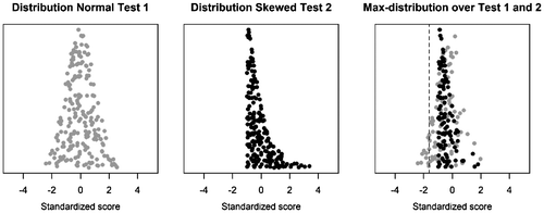
Additionally, the max-approach and stepwise approach require norm group scores to be similarly distributed across tests. If not, tests with skewed distributions may be over- or underrepresented. Figure 1 shows a test with a normal distribution, a test with a skewed distribution, and the max-distribution the pair of tests produce. Herein, only scores from the normally distributed test are represented in the lower tail, beyond the critical value. As such, on the second (skewed) test, the assessed individual requires a score excessively extreme compared to the corresponding test’s norm distribution to be found significant, thus lowering the power. Should norm group test score distributions be found to substantially differ, transforming the data to normality is recommended (de Vent et al., 2016).

Figure 1. Example of how the max-distribution is affected by tests having different distributions; when one test is normally distributed (left), the other is skewed to the right (middle). The dotted line indicates the critical value at α = .05.

In the following paragraph, we outline how we compared these methods in a simulation study.

Data simulation

Data were simulated in R (R Core Team, 2015), with each data-set containing normative data (the norm group) and patient data (the assessed individual). Normative data were simulated as if the data from one or more studies (non-multilevel vs. multilevel data), each containing some or all of the possible tests (no missing data vs. missing data), were merged. In creating the datasets, the following parameters were varied: the number of studies (S), the number of participants per study (N), the number of tests (M), the between-test correlations (BTC), the between-study variance (BSV), and the number of tests in the patient data that showed deviation. Parameter settings were based on the Advanced Neuropsychological Diagnostics Infrastructure (ANDI), a recent initiative in neuropsychological diagnostics containing healthy participant data of various neuropsychological tests, as collected from multiple studies (de Vent et al., 2016; http://www.andi.nl/home).

Number of Tests (M): {1, 2, 3, 5, 15, 24, 50}

The number of administered tests was based on the mean number of tests per study in ANDI, resulting in M = 15; M = 24 was chosen to represent a larger, yet still realistic number of tests. We chose M = 50, as to investigate the effect an extremely large – albeit unrealistic – number of tests had on the analyses. Similarly, M = 2, M = 3, and M = 5 were chosen to investigate hypothetical situations with a relatively small number of tests. Finally, M = 1 served as a baseline, illustrating each method’s performance when multiple testing did not occur.

Number of studies (S): {1, 2, 5, 20, 40}

The mean number of studies in ANDI to include at least one common test was 18, and the largest number was 37. Rounding upwards this became S = 20 and S = 40; S = 1 was included to investigate how each method performed when applied to non-multilevel data; S = 2 and S = 5 were added to examine the effect of multilevel data made up of a small number of studies.

Number of participants per study (N): {10, 20, 70, 200}

The number of participants greatly varies within the ANDI database, as data sources vary from large community samples, to small matched samples in studies about rare diseases. We based our typical sample size on the latter, and chose N = 70. The minimum and maximum number of participants per study of N = 10 and N = 200 were based on the smallest and largest number of participants per study observed in the ANDI data, omitting the large community samples. Data were simulated as if all studies had the same number of participants.

Between-Test Correlations (BTC): {0, .27, .5, .8}

Between-test correlations describe the correlations between tests from the same study; BTC = .27 was the mean between-test correlation in ANDI, and BTC = .8 was the largest between-test correlation. Given the large difference between these values – mostly attributable to the unusually large value of .8 – BTC = .5 was added as to illustrate the effect of high but still common between-test correlations. Additionally, BTC = 0 was chosen to include a situation with completely uncorrelated tests.

Between-Study Variances (BSV):{0, .15, .4}

Between-study variance describes the variance in the norm group data-set attributable to differences between studies, leaving remaining variation attributable to individual differences. These values were based on the intra-class correlations (ICC) found in ANDI; .15 was the mean ICC in ANDI, and .4 the largest ICC found in this dataset. From these correlations, the between-study variances could be computed through the formula: , wherein σ² equals the total variance of the norm group data-set (Tabachnick & Fidell, 2007). In each data-set, σ² was arbitrarily set to 1, resulting in BSV = .15 and BSV = .4. BSV = 0 was included to examine a situation wherein all studies involved were completely equivalent.

Missing data: {0%, 50%}

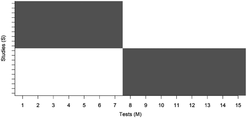
The amount of missing data was set at either 0% (no missing data) or 50% (half of the data were missing). The latter was deemed a sufficiently large percentage to demonstrate the effects of missing data, and was computed by removing scores after data simulation. This was done by removing the first half of the tests (test 1 to M/2) for the first half of the studies (study 1 to S/2), and removing the second half of the tests (test M/2 + 1 to M) from the second half of the studies (study S/2 + 1 to S), as illustrated in Figure 2.

Figure 2. Missing data pattern with 50% of the data missing. Grey areas indicate non-missing values, white areas indicate missing values.

Patient deviation: {1; 5}

The number of tests a patient could deviate on was varied to illustrate the expected increase in power of the stepwise approach over the max-approach in situations with multiple deviating tests. The patient could deviate on either the first, or on the first five tests.

Norm data simulation

The norm group data were simulated as if test scores had already been corrected for demographic influences, meaning they had a mean of zero (de Vent et al., 2016). Thus, the scores of the norm group data only consisted of a within-study term epsilon (ε) and a between-study term denoted by nu (ν). Epsilons differed for each participant and each test. Nu’s differed for each study and each test. By adding these two elements, the test scores were computed: . Epsilons were drawn from a multivariate normal distribution with means of zero and a covariance matrix with variances of 1 − BSV and covariances calculated with the BTC values. Nu’s were drawn from a multivariate normal distribution with means of zero and a covariance matrix with variances of BSV and covariances of 0. Note that because a non-multilevel data-set consists of only one study (S = 1), it should have no between-study variance (BSV = 0), causing the nu’s to equal zero, meaning non-multilevel scores consisted solely of epsilons.

Patient data simulation

Patient data had the same format as the norm data-set, but for N = 1. Patients were either healthy (with scores equaling the mean used in simulating the norm data) or deviant (two standard deviations below the mean used to simulate the normative data, either on the first test or on the first five tests). The inclusion of both healthy and deviant individuals enabled estimation of both the FWER and power of methods. Standard deviations were computed by taking the square root of the respective diagonal element of the summed within-study and between-study covariance matrices. Both the norm data scores and the patient data scores were standardized, as required for the max-approach and stepwise approach.

A total of 1000 data-sets (each consisting of one norm data-set and one patient data-set) were simulated for each type of data, enabling accurate estimation of FWER and power.

Data analysis

For all methods, for each type of norm data-set, the FWER and power were estimated. The FWER was defined as the proportion of healthy patient datasets that were incorrectly identified as deviant – meaning that significant deviation on at least one test (at least one false positive result) was found (Huizenga et al., 2016). The significance threshold was set at α = .05. The power was defined as the proportion of deviant patient data-sets where deviation was correctly identified – meaning that deviation was found on the first test (Malik, Turner, & Sohail, 2015; Parikh, Mathai, Parikh, Sekhar, & Thomas, 2008). This definition of power was maintained regardless of the number of deviating tests.

Results

Results were plotted for the default settings of 70 participants per study, from 20 studies, with 15 tests, with a between-tests correlation of .27, and a between-study variance of .15 (N = 70; S = 20; M = 15; BTC = .27; BSV = .15), unless otherwise noted. These settings were chosen to be typical for the ANDI database. Unless explicitly stated otherwise, no norm data were missing.

Familywise error rate

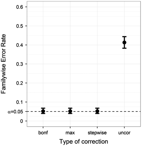
Our first question was whether multiple normative comparisons using a multilevel structured norm group required FWER correction. Figure 3 shows the FWER results for the typical ANDI settings. For uncorrected tests, the FWER results were well above .05, at approximately .40, confirming the necessity of using correction methods. All three correction methods kept the FWER at .05, suggesting adequate correction. Because the FWER of the uncorrected method was so high, this method will not be shown in later figures.

Figure 3. Familywise Error Rate on the y-axis, and type of correction on the x-axis. Plotted for the ANDI-representative settings (N = 70; S = 20; M = 15; BTC = .27; BSV = .15), without missing data. Error bars indicate 95% binomial confidence intervals. The dotted line indicates the significance threshold (α = .05).

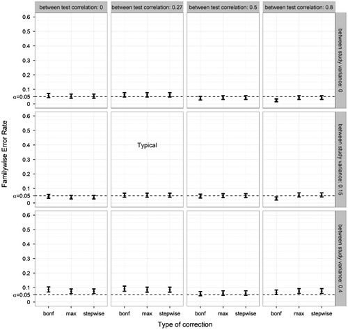
Second, FWER was plotted as a function of between-test correlation (BTC) and between-study variance (BSV), see Figure 4. This revealed that larger between-test correlations resulted in a minor decrease in the Bonferroni correction’s FWER. Between-test correlations had no effect on FWER of the max-approach and stepwise approach. The between-study variance had a small effect on the FWER, where a high between-study variance increased the FWER to slightly above .05 across methods. The uncorrected method produced FWER values between .157 (BTC = .8; BSV = 0) and .567 (BTC = 0; BSV = .15).

Figure 4. Familywise Error Rate on the y-axis, and type of correction on the x-axis. Plotted for various combinations of correlations between tests and various variances between studies (other parameters fixed at ANDI-representative settings: N = 70; S = 20; M = 15), without missing data. Error bars indicate 95% binomial confidence intervals. The dotted lines indicate the significance threshold (α = .05). The graph marked by ‘Typical’ denotes that the between-test correlation and between-study variance corresponded to ANDI-representative settings (BTC = .27; BSV = .15).

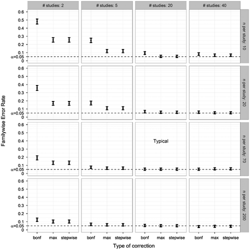
Third, we looked at the influence of sample size on FWER. Sample size could either be changed by changing the number of studies (S), or by changing the number of participants per study (N). In Figure 5, different combinations of these two factors are shown. With a high sample size all three methods produced FWERs of .05, but increased FWER values were found as the sample size decreased; herein, decreasing the number of studies had a more pronounced effect than decreasing the number of participants per study. Noticeably, the Bonferroni correction produced a higher FWER than the other two methods when the number of participants was low. The uncorrected method showed FWER values between .396 (S = 40; N = 200) and .636 (S = 2; N = 10).

Figure 5. Familywise Error Rate on the y-axis, and type of correction on the x-axis. Plotted for various combinations of number of studies and number of participants per study (other parameters fixed at ANDI-representative settings: M = 15; BTC = .27; BSV = .15), without missing data. Error bars indicate 95% binomial confidence intervals. The dotted lines indicate the significance threshold (α = .05). The graph marked by ‘Typical’ denotes that the number of studies and participants per study corresponded to ANDI-representative settings (S = 20; N = 70).

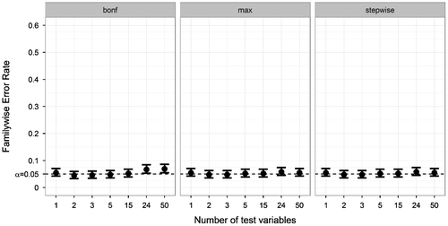
Fourth, we looked at the influence of the number of tests (M). The FWER of all correction methods for several numbers of tests was plotted in Figure 6. For the Bonferroni correction, the FWER became elevated for 24 tests or more. The max-approach and stepwise approach showed no increased FWER. As expected, the uncorrected method showed a strong FWER increase as a result of multiple testing, with FWER = .055 (M = 1) to FWER = .719 (M = 50).

Figure 6. Familywise Error Rate on the y-axis, and number of tests on the x-axis. Plotted for various numbers of tests (other parameters fixed at ANDI-representative settings: N = 70; S = 20; BTC = .27; BSV = .15), without missing data. Error bars indicate 95% binomial confidence intervals. The dotted line indicates the significance threshold (α = .05).

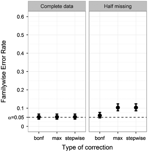
Fifth, we looked at the influence of missing data. Figure 7 displays the FWER of the three correction methods with either complete data or 50% of the data missing. Both the max-approach and the stepwise approach showed an increased FWER when missing data were introduced. The Bonferroni correction showed a negligibly small FWER increase. The uncorrected method appeared almost unaffected by missing data, with FWER = .42 (complete data) and FWER = .413 (missing data).

Figure 7. Familywise Error Rate on the y-axis, and type of correction on the x-axis. Plotted for both complete data (left) and data with half of the values removed (right), only for the ANDI-representative settings (N = 70; S = 20; M = 15; BTC = .27; BSV = .15). Error bars indicate 95% binomial confidence intervals. The dotted line indicates the significance threshold (α = .05).

To summarize, FWER analysis revealed that the uncorrected method consistently produced FWER values above .05. This confirmed that performing multiple normative comparisons using multilevel data requires FWER correction. All correction methods produced better FWER values across a variety of situations. Between-test correlations slightly affected the FWER of the Bonferroni method, but not the FWER of the other correction methods. Between-study variance did affect FWER, with higher variances producing an increased FWER across correction methods, though only with relatively large between-study variances – which would be rare in clinical practice – and even then the increase was very mild. The number of tests only affected the Bonferroni correction, causing a small FWER increase as the number of tests increased. All correction methods showed an elevated FWER when the norm group was small, with the Bonferroni correction suffering most, especially when the number of participants was low. Missing data caused an increased FWER in the max-approach and stepwise approach alone. In short, the max-approach and stepwise approach outperformed the Bonferroni correction, especially when the norm data contained a low number of studies, or when the number of tests was high. Only when the norm data contained missing values, did the Bonferroni correction outperform the other correction methods.

Power

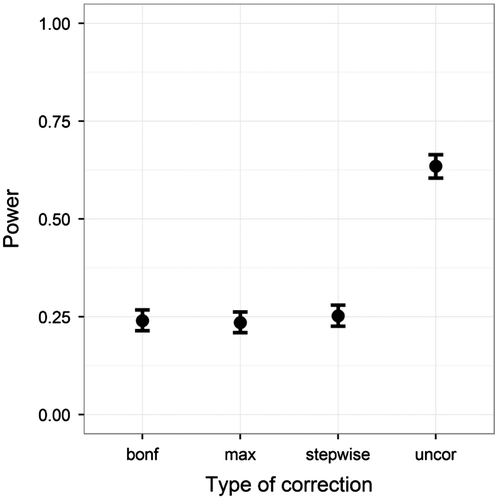
First, we looked at the power when the patient data deviated on the first test only, using the ANDI-representative settings (N = 70; S = 20; M = 15; BTC = .27; BSV = .15). The power of the three correction methods and uncorrected normative comparison was plotted in Figure 8. The uncorrected method had the highest power. The three FWER correction methods produced almost identical results, and thus were concluded not to differ amongst each other.

Figure 8. Power on the y-axis, and type of correction on the x-axis. Plotted for the ANDI-representative setting (N = 70; S = 20; M = 15; BTC = .27; BSV = .15), without missing data. Error bars indicate 95% binomial confidence intervals.

Next, we looked at the power when the patient data deviated on the first five tests. Recall that power calculations only identified deviation on the first test. Figure 9 displays the power of all four methods while varying the correlations between tests. The uncorrected method still produced the highest power. Out of the correction methods, the stepwise approach had the highest power – even approximating the power of the uncorrected method, especially at low between-test correlations. The max-approach behaved in an opposite manner, showing increased power as between-test correlations increased, though never outperforming the stepwise approach. The Bonferroni method showed a consistently low power across between-test correlations.

Figure 9. Power on the y-axis, and type of correction on the x-axis. Five deviations were simulated. Power was estimated as proportion of significant deviations found on the first test. Plotted for various between-tests correlations (other parameters fixed at ANDI-representative settings: N = 70; S = 20; M = 15; BSV = .15), without missing data. Error bars indicate 95% binomial confidence intervals.

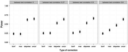
To summarize, the uncorrected method produced the highest power. Unfortunately, this held little relevance as this method was already shown to fail in terms of FWER criteria. Out of the correction methods, the stepwise approach excelled when the assessed individual deviated on multiple tests. This agrees with the idea that both the Bonferroni and the max-approach are unfairly restrictive, especially for all except the most deviating test scores. Also, in neuropsychological assessment deviation on multiple tests is to be expected, as cognitive functions are correlated. As such, this advantage of the stepwise approach makes it very useful for clinical practice.

Other combinations of data simulation parameters that were varied are also available; all simulation results are provided online.³

Discussion

This study examined the assessment accuracy of several normative comparison methods when the norm group data were obtained from an aggregated data-set. The goal was to determine which method would be most suitable for use in neuropsychological assessment. Uncorrected normative comparison, and three FWER correction normative comparison methods – the Bonferroni correction, the max-approach, and the stepwise approach – were tested. Good assessment accuracy was defined as a familywise error rate (FWER) not exceeding the preset significance threshold. Additionally, the power was aimed to be as high as possible.

The uncorrected method consistently produced too high FWER values, meaning it too often untruthfully indicated that the assessed individual deviated from the norm group. The correction methods were shown to reduce the FWER. Several data parameters were varied to examine which correction method performed best under different circumstances. When the norm group contained many missing data, the Bonferroni correction controlled the FWER better than the max-approach and stepwise approach. Without missing data the stepwise approach performed preferably, as it had equivalent or better control over the FWER, and an equivalent or higher power across a variety of situations. This was especially pronounced in situations with a smaller number of studies or participants, situations with a higher number of tests, and when between-test correlations were low.

Several points require discussion. First, the max-approach and stepwise approach performed well as long as the norm group contained a sufficient amount of studies, while the Bonferroni correction suffered when either the number of studies or the number of participants was reduced. This difference can be explained by the fact that reducing norm group size results in fewer data points to make up the norm group distribution. Especially the tails of the distribution are affected by this, as they contain few data points to begin with. This affects the Bonferroni correction most because it implements a lower significance threshold for each test, and a lower threshold directs the comparison towards the most extreme part of the distribution (essentially the tail of the tail), which contains even fewer scores, and is thus even more affected by decreased sample size.

Second, introducing missing data to the norm group data-set led to an increased FWER in the max-approach and stepwise approach, but did not substantially affect the Bonferroni correction. This can be explained by the former two methods constructing norm group distributions by selecting extreme scores across tests; when half of the tests are missing these distributions may become too narrow (i.e. not critical enough). The Bonferroni correction isn’t affected as it does not use the extreme values over all tests to make a new distribution to which the patient scores are compared.

Third, the stepwise approach produced a much higher power than the other correction methods when multiple tests deviated, especially when between-test correlations were low. This may be explained by the stepwise approach computing different distributions for each test score. More extreme scores are compared to more extreme distributions – distributions made up of the most extreme norm group scores. When tests are highly correlated, extreme scores on one test come with extreme scores on other tests, meaning there are more extreme scores in total. Thus the distributions become more critical, making it harder to detect deviation, thus reducing power.

Fourth, despite the stepwise approach yielding higher power than Bonferroni correction or max-approach, it occasionally produced a low power, which may spark reluctance to use it in clinical practice. However, the stepwise approach still outperformed the Bonferroni correction, and while the uncorrected method consistently produced the highest power, it also produced a highly increased FWER. It is the overall accuracy, the combination of a low FWER and relatively high power that makes the stepwise approach most suitable for practical application. When high(er) power is preferred, we recommend a more liberal threshold (e.g. α = .20 instead of α = .05). This has the advantage of the true FWER being known (i.e. when the significance threshold of the stepwise approach is set to α = .20, the resulting FWER will approximate .20), whereas using the uncorrected comparisons will produce an FWER increase of an unknown extent.

Fifth, norm data were simulated so that the number of participants was equal across studies, which is unlikely to occur in real aggregated data. A post hoc simulation study with unequal sample sizes (using the default settings) showed similar patterns in terms of FWER results as it did with equal sample sizes.

Sixth, due to this being a simulation study, generalizability of results may be called into question. However, data simulation allowed for the examination of each method’s performance under many different circumstances, thus boosting generalizability. More importantly, simulation parameters were based on real data to enhance generalizability, leading us to believe that these results are representative of real life situations.

Finally, it must be stressed that none of the discussed statistical methods are meant to be the sole basis of diagnosis, with contextual information and the assessors’ professional opinion playing an important role – both in interpreting analysis results and in translating them into a meaningful judgment and effective treatment.

Practical advice

When the norm data contain no missing data, the stepwise approach appears to be the most suitable method for normative comparison with an aggregated norm group; it best corrects the increased FWER associated with multiple testing, with FWER least affected by the properties of the norm group. Moreover, it produces a relatively high power when the assessed individual deviates on multiple tests. Based on this, we recommend the stepwise approach as the default method for neuropsychological assessment with an aggregated normative database. However, when the norm data contains (large portions of) missing data – for example, when several of the administered tests are relatively uncommon – the Bonferroni corrections should be preferred.

Also, when the norm group sample size is small, neither correction method performs well. In such instances, we recommend the resampling-based normative comparison methods from Huizenga et al. (2016). These methods were made specifically with small norm groups in mind, and proved to have good assessment accuracy with small sample sizes (Huizenga et al., 2016; Li & Dye, 2013; Troendle, 1995). However, note that these methods have not yet been tested for multilevel data or norm groups with missing data.

The uncorrected method, the Bonferroni correction, the max-approach and stepwise approach have been implemented in a freely available online app (see: https://joost.shinyapps.io/EmpiricalNormComp/).

Final comments

FWER corrections are needed in neuropsychological assessment when performing more than one normative comparison. In this simulation study, we have shown that correcting multiple comparisons using the stepwise approach can be a useful alternative to Bonferroni corrections when using aggregated norm data. We hope that this leads to a broader adoption of correction methods, as it is important to reduce the number of false positives in clinical practice, while remaining sensitive to true deviations.

Author contributions

HMH, JAR, JNZ developed the study concept, design, and method. Data simulation, analysis, and reporting were done by JAR, JNZ. The manuscript was drafted by JNZ, with critical revisions by HMH and JAR. All authors approved the final version of the manuscript for submission.

Disclosure statement

No potential conflict of interest was reported by the authors.

Funding

This work was supported by a VICI [grant number 453–12-005]; and a MaGW [grant number 480–12-015] awarded by the Dutch Science Foundation (NWO).

Notes

1. In the current setting, with a large sample size, we do not need test statistics, but can instead work with the raw percentiles as is done in many test manuals.

2. An added restriction (referred to as the ‘monotonicity assumption’) is that less extreme scores are not allowed to produce lower p-values than more extreme scores, and if this occurs the p-value of the less extreme score is set to equal that of the more extreme score. This implements the logical assumption that less extreme scores cannot produce more significant results (Gordon, 2011).

3. See: https://raw.githubusercontent.com/JAvRZ/SupplementalMaterialUnivariateNormativeComparisons/master/Simulationdata.csv

References

- Agelink van Rentergem, J. A., de Vent, N. R., Schmand, B.A., Murre, J. M. J., & Huizenga, H. M. (in press). Multivariate normative comparisons for neuropsychological assessment by a multilevel factor structure or multiple imputation approach. Psychological Assessment.
- Agelink van Rentergem, J. A., Murre, J. M. J., & Huizenga, H. M. (2017). Multivariate normative comparisons using an aggregated database. PLoS ONE, 12, 1–18.
- Armstrong, R. A. (2014). When to use the Bonferroni correction. Ophthalmic and Physiological Optics, 34, 502–508. doi:10.1111/opo.12131.
- Asendorpf, J. B., Conner, M., De Fruyt, F., De Houwer, J., Denissen, J. J., Fiedler, K., … Perugini, M. (2013). Recommendations for increasing replicability in psychology. European Journal of Personality, 27, 108–119. doi:10.1002/per.1919
- Binder, L. M., Iverson, G. L., & Brooks, B. L. (2009). To err is human: “Abnormal” neuropsychological scores and variability are common in healthy adults. Archives of Clinical Neuropsychology, 24, 31–46. doi:10.1093/arclin/acn001
- Blakesley, R. E., Mazumdar, S., Dew, M. A., Houck, P. R., Tang, G., Reynolds, C. F., III, & Butters, M. A. (2009). Comparisons of methods for multiple hypothesis testing in neuropsychological research. Neuropsychology, 23, 255–264. doi:10.1037/a0012850
- Bland, J. M., & Altman, D. G. (1995). Statistics notes: Multiple significance tests: The Bonferroni method. BMJ, 310, 170. doi:10.1136/bmj.310.6973.170
- Cao, J., & Zhang, S. (2014). Multiple comparison procedures. JAMA, 312, 543–544. doi:10.1001/jama.2014.9440
- Crawford, J. R., & Howell, D. C. (1998). Comparing an individual’s test score against norms derived from small samples. The Clinical Neuropsychologist (Neuropsychology, Development and Cognition: Section D), 12, 482–486.10.1076/clin.12.4.482.7241
- Dupont, W. D., & Plummer, W. D. (1990). Power and sample size calculations. Controlled Clinical Trials, 11, 116–128.10.1016/0197-2456(90)90005-M
- Feise, R. J. (2002). Do multiple outcome measures require p-value adjustment? BMC Medical Research Methodology, 2(1), 1. doi:10.1186/1471-2288-2-8
- Field, A. (2009). Discovering statistics using SPSS (3rd ed.). London: SAGE publications.
- Gordon, A. Y. (2011). A new optimality property of the Holm step-down procedure. Statistical Methodology, 8, 129–135. doi:10.1016/j.stamet.2010.08.003
- Gordon, A. Y., & Salzman, P. (2008). Optimality of the Holm procedure among general step-down multiple testing procedures. Statistics & Probability Letters, 78, 1878–1884. doi:10.1016/j.spl.2008.01.055
- Harvey, P. D. (2012). Clinical applications of neuropsychological assessment. Dialogues in Clinical Neuroscience, 14, 91–99.
- Holm, S. (1979). A simple sequentially rejective multiple test procedure. Scandinavian Journal of Statistics, 6, 65–70.
- Huizenga, H., Agelink van Rentergem, J., Grasman, R., Muslimovic, D., & Schmand, B. (2016). Normative comparisons for large neuropsychological test batteries: User-friendly and sensitive solutions to minimize familywise false positives. Journal of Clinical and Experimental Neuropsychology, 38, 611–629. doi:10.1080/13803395.2015.1132299
- Huizenga, H. M., Smeding, H., Grasman, R. P., & Schmand, B. (2007). Multivariate normative comparisons. Neuropsychologia, 45, 2534–2542. doi:10.1016/j.neuropsychologia.2007.03.011
- Kendall, P. C., Marrs-Garcia, A., Nath, S. R., & Sheldrick, R. C. (1999). Normative comparisons for the evaluation of clinical significance. Journal of Consulting and Clinical Psychology, 67, 285–299.10.1037/0022-006X.67.3.285
- King, G. (2011). Ensuring the data-rich future of the social sciences. Science, 331, 719–721. doi:10.1126/science.1197872
- Lezak, M. D., Howieson, D. B., Bigler, E. D., & Tranel, D. (2012). Neuropsychological assessment (5th ed.). New York, NY: Oxford University Press.
- Li, D., & Dye, T. D. (2013). Power and stability properties of resampling-based multiple testing procedures with applications to gene oncology studies. Computational and Mathematical Methods in Medicine, 2013, doi:10.1155/2013/610297
- Malik, A. B., Turner, M. E., & Sohail, M. (2015, March 11). Neuropsychological evaluation. Retrieved February 22, 2016, from https://emedicine.medscape.com/article/317596-overview#a8.
- Moran, M. D. (2003). Arguments for rejecting the sequential Bonferroni in ecological studies. Oikos, 100, 403–405. doi:10.1034/j.1600-0706.2003.12010.x
- Narum, S. R. (2006). Beyond Bonferroni: Less conservative analyses for conservation genetics. Conservation Genetics, 7, 783–787. doi:10.1007/s10592-005-9056-y
- Nichols, T. E., & Holmes, A. P. (2002). Nonparametric permutation tests for functional neuroimaging: A primer with examples. Human Brain Mapping, 15(1), 1–25.10.1002/(ISSN)1097-0193
- Parikh, R., Mathai, A., Parikh, S., Sekhar, G. C., & Thomas, R. (2008). Understanding and using sensitivity, specificity and predictive values. Indian Journal of Ophthalmology, 56, 45–50. doi:10.4103/0301-4738.37595
- Poline, J. B., Breeze, J. L., Ghosh, S., Gorgolewski, K., Halchenko, Y. O., Hanke, M., … Poldrack, R. A. (2012). Data sharing in neuroimaging research. Frontiers in Neuroinformatics, 6–9, doi:10.3389/fninf.2012.00009
- R Core Team. (2015). R: A language and environment for statistical computing. Vienna: R Foundation for Statistical Computing. Retrieved from https://www.R-project.org/.
- Steenbergen, M. R., & Jones, B. S. (2002). Modeling multilevel data structures. American Journal of Political Science, 218–237, doi:10.2307/3088424
- Tabachnick, B. G., & Fidell, L. S. (2007). Using multivariate statistics (5th ed.). Boston, MA: Pearson Education.
- Troendle, J. F. (1995). A stepwise resampling method of multiple hypothesis testing. Journal of the American Statistical Association, 90, 370–378.10.1080/01621459.1995.10476522
- Van der Laan, M. J., Dudoit, S., & Pollard, K. S. (2004). Multiple testing. Part II. Step-down procedures for control of the family-wise error rate. Statistical Applications in Genetics and Molecular Biology, 3(1), 1–33. doi:10.2202/1544-6115.1041
- de Vent, N. R., Agelink van Rentergem, J. A., Schmand, B. A., Murre, J. M. J., ANDI Consortium, & Huizenga, H. M. (2016). Advanced Neuropsychological Diagnostics Infrastructure (ANDI): A normative database created from control datasets. Frontiers in Psychology, 7, 1601. doi:10.3389/fpsyg.2016.01601
- Verhoeven, K. J., Simonsen, K. L., & McIntyre, L. M. (2005). Implementing false discovery rate control: Increasing your power. Oikos, 108, 643–647. doi:10.1111/j.0030-1299.2005.13727.x
- Vines, T. H., Albert, A. Y., Andrew, R. L., Débarre, F., Bock, D. G., Franklin, M. T., … Rennison, D. J. (2014). The availability of research data declines rapidly with article age. Current Biology, 24, 94–97. doi:10.1016/j.cub.2013.11.014
- Westfall, P. H., & Young, S. S. (1993). Resampling-based multiple testing: Examples and methods for p-value adjustment (Vol. 279). Hoboken, NJ: Wiley.