A lattice gas model with temperature and buoyancy effects to predict the concentration of pollutant gas released by power plants and traffic sources

Abstract

A method to simulate the dispersion of pollutant gases in the air, which is based on the lattice gas technique, is presented. The model is able to represent the main transient and local effects, thus it is an alternative to the direct numerical simulation of the turbulent diffusion paths. No parametrization of the turbulence is needed, nor of the momentum and energy exchange between the pollutant and the air. Few non-dimensional parameters define completely the case to study. The predictions of the model, including the buoyancy effects, are compared in the steady-state limit with the Gaussian plume equation. The effective values of the dispersion coefficients and of the plume rise height are extracted from the results and are compared with the values resulting from the application of the most widely used semi-empirical correlations.

Keywords:

• Pollutant gas dispersion
• Stack emissions
• Lattice gas model
• Cellular automata

1 Introduction

The lattice gas technique, which represents a particular class of cellular automata, has been proposed for two decades for the simulation of various fluid dynamics processes [1,2]. In this approach, the fluids are represented by fictitious particles that move across the sites of a regular lattice, obeying simple rules for transport, collisions, interactions with obstacles, etc. With respect to computational fluid dynamics, there is no need for complex solution algorithms, and the definition of the model parameters is simpler and less subject to uncertainties. It has also been proved that, for particular classes of problems and on an average basis, the lattice gas shows the same behaviour as described by the classical differential equations used to represent the process under investigation. Further details on the development and the features of this technique can be found in [3 –  5].

One of the first attempts to use a lattice gas for the dispersion of gaseous pollutants emitted from stack sources can be found in the work by Salcido [6,7]. Salcido showed how the lattice gas rules, in spite of their relative simplicity, are sufficient to simulate, at least qualitatively, some complex processes affecting unsteady dispersion, including momentum exchange with the surrounding atmosphere and deposition. A comprehensive stochastic lattice gas model, which was built in order to provide also reliable quantitative predictions, was presented in [8,9]. The obtained model responses were shown to be compatible with those yielded by the Gaussian plume equation (GPE), in the GPE's limits of steady-state and fully developed plumes.

These first applications all dealt with non-thermal plumes, this is, the buoyancy effects were not considered. In general, it is a problem of the lattice gas models that temperature is not easily represented by means of particles moving across a lattice. Various approaches have been proposed, some of which have been recognized as unrealistic [10], and others seem to be too complex for practical and quantitative calculations [11].

In this work, two ways to represent the thermal effects are investigated: a statistical approach and a kinetic approach. The latter is selected owing to its simplicity and because it fits particularly the case in which there are few pollutant particles in the surrounding air, which is the case of transient emission. With the new feature, it is possible to simulate the buoyancy effects and the influence of different air temperature profiles.

First a detailed overview of the model is presented, with the automata rules described formally in terms of mathematical operators. Section 2 includes a discussion of the derivation of a relationship for the temperature and how this is applied in the model. The results presented in section 3 concern the evaluation of the plume rise and the capability of the model to treat different air temperature profiles.

2 The lattice gas model

The model adopts the modified Hardy – de Pazzis – Pomeau (HPP) [1] lattice gas. According to this model, the fluid particles can move across the four directions of a square lattice (in two dimensions), or they may be at rest. This model was chosen for its simplicity, in spite of its inherent anisotropy which was considered to yield effects that are quantitatively negligible. A difference with respect to the original formulation of the HPP is that the model is not deterministic, that is most of the rules for the motion of the particles include randomness.

2.1 Definition of the lattice

The fictitious particles describing the air and the pollutant reside on a two-dimensional lattice with square cells of fixed dimension Δr. The two species of particles have identical masses Δm. The third dimensional parameter that defines the study case is the time step Δt of the solution. In [9] the influence of the lattice parameters on the solution was investigated. Three non-dimensional numbers have been conveniently defined as a combination of physical quantities: Δr, Δm and Δt. Heuristic observations on the model's behaviour suggested that the average number of particles per site (defined in [9] as the ‘number ratio’ X_n ) mainly influences the lateral diffusion, the non-dimensional characteristic time (the ‘time ratio’ X_t ) only weakly influences the vertical diffusion, while the non-dimensional characteristic velocity (the ‘velocity ratio’ X_u ) does not have a significant influence on the process simulated. Thus X_n and, to a lesser extent, X_t should be regarded as tuneable parameters.

2.2 Microdynamics

The particles can move only from one lattice site to the four nearest neighbours or be at rest. Consequently, the velocity in the lattice units c is quantized to have five values: c _k  = [cos [(π/4)(k − 1)]], [sin[(π/4)(k−1)]], k = 1,…,4, c ₅ = [0,0]. The physical velocity is (Δr/Δt) c .

The Boolean quantities that describe the particle occupation of the site x at time t are n_k ( x ,t) for the pollutant particles and u_k ( x ,t) for the air particles (k = 1,.…,5). Both of these quantities have a value of 1 when there is a particle with direction k, or 0 when there is not.

The distribution u_k ( x ,t) is assigned at each time t, in order to respect a given wind field. The spatial domain is divided in a number of sets Z, each of them containing the β(z) sites at the same height z. For each height, the air density ρ(z) and the wind speed v (z) are given. Then, the particles are assigned to the sites randomly, in such a way that

where k _B plays the role of the Boltzmann constant, that is the proportionality factor between the temperature θ and the internal energy; (3) is derived from the kinetic definition of temperature that has been adopted:

The alternative choice is a statistical definition of temperature, formally written as k _Bθ = f_θ (e,υ, p ,β). This possibility was investigated (see next section) but finally abandoned as being unpractical.

2.3 The lattice gas temperature

The relationship k _Bθ = f_θ (e,υ, p ,β) is derived by applying the definition of temperature of a thermodynamic gas:

In this equation, σ is a non-dimensional entropy, defined as σ = logW, where W = W(e,υ,π,β), the total number of configurations possible. The momentum is written as p  = [π_x ,π_z ] where π = |π_x | = |π_z |. The expression that has been derived for W, valid for the case considered of a lattice gas with five allowed directions, is:

where ν _i  = (e−π)/2 is the excess of particles moving but not contributing to the net momentum.

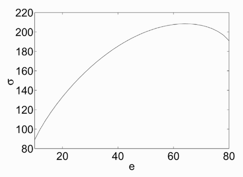
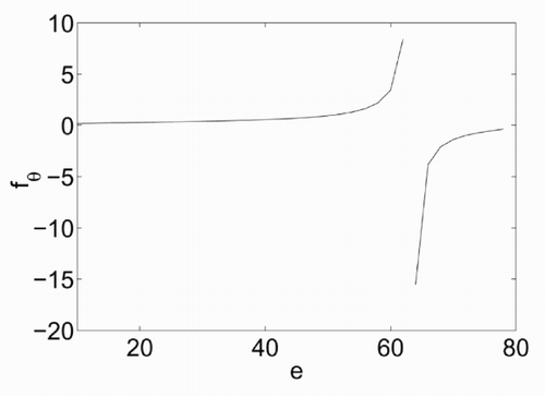
The dependence of σ on e is illustrated in figure 1, which has been derived for ν = 80, π = 10, β = 100 and e ranging from π to ν. The curve σ = σ(e) shows a maximum at a value of energy that will be denoted as e ₀. At this value, the derivative of σ with respect to e is zero, which means that, based on (5), the temperature θ tends to infinity. The dependence of f_θ on e is shown in figure 2. There are two branches of this curve, at both sides of e = e ₀. The resulting temperature is positive only for the left branch. A non-physical negative temperature is obtained instead for e > e _0.

Figure 1. Dependence of the non-dimensional entropy σ on the lattice energy e.

Figure 2. Dependence of the temperature function f_θ on the lattice energy e.

The curve f_θ  = f_θ (e) has been derived via numerical differentiation. To derive an analytical relationship that is easy to handle, first the summation

in (6) is replaced by ν_iW_j0 , that is the mean value evaluated at the energy index j₀ , multiplied by the range of j:

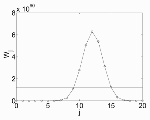
This procedure is clarified by figure 3, which shows the various W_j as a function of j, for a given energy e = 50, which corresponds to ν_i  = 20. The curve has a peak for j = 12. Also shown is the mean value

, which can be approximated by two values of W_{j 0}, at the two sides of the curve peak. In general, the value j ₀ considered here is that on the decreasing branch of the curve. For example, with the value of e mentioned, it is j ₀ = 11.

Figure 3. Dependence of the terms W_j (○) in (6) on the index j, mean value of W_j .

The influences of β,ν,e and π on the value j ₀ can be hardly determined a priori or on the basis of analytical considerations. Instead, a heuristic approach has been adopted, consisting in varying the influence parameters above and observing the result in terms of j ₀. The following results have been found.

	The number β of sites does not significantly influence the relationship fθ , nor does the evaluation of j 0. This is in agreement with the property of the thermodynamic gases that the temperature is a function only of the energy and not of the volume.
	The value of j 0 does not depend on ν, but only on e and π.
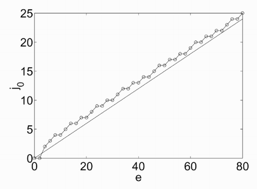
	The dependence of j 0 on e, for π = 0, is shown in figure 4. It is a good approximation of a linear dependence with a coefficient of 0.3. The differences between the two curves arise mainly because both e and j 0 are integers.
	The dependence of j 0 on π is nonlinear but can be handled considering that for π = 0 it is j 0 = 0.3e (for the point above), and for π = e it has to be j 0 = 0 (since υi = 0 in this case).

Figure 4. Values of j ₀ as a function of the energy e for π = 0 (○), linear approximation j ₀ = 0.3e.

Summarizing, a close equation found for j ₀ is

Then, the derivative of σ = log(W) with respect to e is calculated, using the approximation:

The resulting equation is

which yields the sought relationship k _Bθ = f_θ (e,ν, p ,β). In figure 5 the quantity 1/f_θ as evaluated with (10) is compared with the values given by the numerical differentiation of (5) and (6) for the same values of β and ν as in figure 3 and for different values of π, ranging from 0 to υ. The agreement is quite good for π close to zero, while the difference between the two curves increases with π approaching ν. Similar results have been obtained for other values of ν (again, with β having no influence).

Figure 5. Dependence of 1/f _θ on the energy e, numerical (x) and approximated (○), for different values of π = 0,…,70.

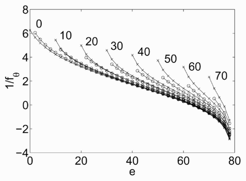
The main advantage of a statistical definition of temperature would be the absence of limits for θ. In contrast, (4) deals with a finite energy spectrum, and consequently only a bounded set of possible values of θ can be represented.

Unfortunately, the statistical definition of temperature has been derived and thus it is reliable only for a sufficiently large number of particles. This is the case of the air field in (1) but, as for the pollutant emission, more often the contrary is true; that is, during transient emissions, the number of particles released is small. For this reason, (4) was applied in the model.

2.4 Rules of particle motion

The distribution of pollutant particles, n_k ( x ,t), is determined from the application of the seven rules illustrated below. In the following, the function δ(·) is defined as

2.4.1 Release

The pollutant particles are introduced in the lattice at the site x _e that corresponds to the source. The emission is random but, over a large time τ, it respects the physical mass flow rate

, velocity v _e and temperature θ_e:

2.4.2 Transport

The first rule to be applied at the beginning of a new time step t + Δt is that each particle moves from the site x occupied at time t to one of its nearest neighbours or keeps at rest, according to its velocity c :

2.4.3 Principle of exclusion

After having moved the pollutant particles according to the previous rule and having reassigned the air particles, if at a certain site there are one pollutant particle and one air particle that move in the same direction, then the air particle is removed and redistributed in a ‘free’ site at the same height z, preserving its direction k. In terms of Boolean variables, this rule can be written as

where a tilde means logical negation and all the Boolean variables are taken implicitly at time t and site x . After having applied this rule, it means n_ku_k = 0 for the rest of the current time step, and therefore the new variable x_k ≡ n_k  + u_k will also be Boolean.

2.4.4 Collisions involving pollutant particles

If at a certain site there is more than one particle, with at least one pollutant particle, then a collision occurs. The Σ _kn_k particles of pollutant, and the Σ _kn_k particles of air involved in the collision are redistributed at the same site, preserving the total momentum and energy. The pollutant distribution after the collisions is described by the equation

for k = 1,…,4 (each subscript is modulo 4), and

Again, all the Boolean variables are taken implicitly at time t and site x .

2.4.5 Buoyancy force

The application of the buoyancy force to the pollutant particles requires the evaluation of the temperature difference between the pollutant particles and the air particles that occupy the same sites. For convenience the spatial domain is divided into a number of ‘observation domains’, each of them including 4 × 4 sites. For each domain, a local contribution to the overall temperature difference is evaluated by summation over the sites x ∈D which are occupied by at least one pollutant particle:

where

is a reference air temperature taken at the source height.

Then, the total positive and negative variations in the pollutant momentum due to the buoyancy force are evaluated as

These quantities are applied by inverting the motion of

pollutant particles with direction k = 4 to k = 2 and the motion of

pollutant particles with direction k = 2 to k = 4. In fact, each particle affected contributes to the total variation of momentum with a quantity of 2, in lattice units. Such particles are randomly selected. In terms of Boolean variables, it is

for k = 2,4 (k is modulo 4), otherwise the distribution n_k is not affected. The set R₂ is the union of all the domains D such that θ_D  > 0, while R ₄ is the union of all the domains D such that θ_D  < 0. The auxiliary Boolean variable d_k is true when x ∈R_k .

2.4.6 Boundaries

Three types of lattice boundary are considered: absorbing, transparent and reflecting. The first can be the case of the ground, the second fits the limits of the lattice that do not correspond to any physical barrier, while the third can be associated with mixing height. In the first case, the rule to be applied in terms of Boolean distribution is simply

for the direction k perpendicular to the boundary. In the case of the reflecting boundary, it is

again for the direction k perpendicular to the boundary, and k cyclic (modulo 4). The transparent lattice boundary can be considered an intermediate case between these two extremes. Then, a ‘virtual source’ is added (as for the reflecting case) or subtracted (as for the absorbing case) with probability one half. In terms of Boolean distribution, this can be written as

2.5 Concentration field

The pollutant concentration is evaluated as a time average, with the following equation:

3 Results

In this section, some typical simulations of the lattice gas are presented, leading to the evaluation of the concentration field in a given spatial domain. A basic test case has been considered: an emission from a single point source in a rectangular domain 400 m × 300 m, delimited by the horizontal ground and characterized by a constant horizontal wind. The data for this case are listed in table 1. The values for the model parameters are Δr = 3 m, Δt = 0.3 s and Δm = 8 kg (X_n  = 1.41, X_t  = 1.06 and X_u  = 0.70). Simulation time runs 2 – 3 slower than real time on a Pentium III, 750 MHz machine.

Table 1. Data for the basic test.

υ a	3.5 m/s	υ e	7 m/s
A e	3 m^2	h e	30 m
θ a	295 K	ρ e	1.19 kg/m^3

The results of the model are compared in the steady-state limit with those calculated with the GPE which, for the case studied, is written as

where σ_y and σ_z are the lateral and vertical dispersion coefficients respectively and x _r is the position of the ‘effective’ source, that is the geometrical source x _e elevated by the height of the plume rise. This equation is valid for transparent boundaries. The general formulation for the dispersion coefficients adopted here is σ_y  = α and σ_z  = γx ^δ . The reason for the first of these relations is that the lateral dispersion is uniform for a two-dimensional lattice. In other words, the model simulates the dispersion in a ‘canyon valley’ of width Δr. The relationship for σ_z has been selected because it is easy to parametrize and because data for the coefficients are available from many sources.

3.1 Plume without thermal effects

The first case presented is one in which the two models are directly comparable. In the GPE the evaluation of the plume rise is simply made by assigning the stationary rise height, whose calculation is then decoupled from the evaluation of the dispersion paths. In contrast, as the lattice gas model is a fluid-dynamics simulator, the plume rise is a consequence of the rules of the particle motion implemented. The kinetic rise derives from the momentum exchange with the surrounding air particles due to collisions. The thermal rise derives from the buoyancy force. However, for a strict comparison with the GPE, a case without plume rise was needed. In order to simulate a process in which the plume axis is steady at the emission source, the calculation of the buoyancy force (no thermal plume rise) in the lattice gas model was suppressed artificially. Moreover, the emission velocity was set to zero (no kinetic plume rise), while keeping the mass flow rate at the value resulting from the data in table 1.

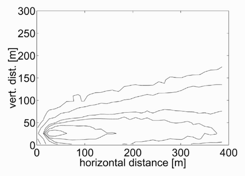
The result obtained is shown in figure 6 in terms of isoconcentration lines in the plane x–z. This result is calculated at steady state, that is after 600 s from the start of the emission. It is evident that the model can represent the main processes. The concentration curves have the typical shape of a plume, with higher concentrations around the source (placed at x _e = [30,30] in the Cartesian domain) and then decreasing with the downwind distance. Since the wind profile is constant, the concentration contours are rather symmetrical with respect to an axis. Coherently with the aim of this test, this plume axis seems reasonably close to the source height. For all these aspects, the concentration contours are in qualitative agreement with those that can be obtained with the GPE.

Figure 6. Concentration contour plot for the basic test without plume rise.

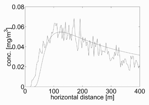
Looking for a quantitative equivalence between the two models, the three dispersion parameters α, γ and δ were varied and the corresponding results of the GPE were compared with those in figure 6. A combination of values which seemed correct was α = 0.35, γ = 0.6, δ = 0.79. Figure 7 shows the concentration calculated at the ground as a function of the downwind distance for the two models. A comparison of the amplitude and the downwind position of the concentration peak shows that the equivalence is satisfactory, also considering the inherent fluctuations of the lattice gas model, which are due to the randomness involved. Note that the values selected for the dispersion coefficients are in the range provided by the classical empirical relationships widely used in practice (see, for example, [12 –  14]).

Figure 7. Concentration as a function of the downwind distance for the basic test without plume rise, GPE (smooth curve) and lattice gas model (non-smooth curve).

3.2 Effect of the temperature gradient

Next, the sensitivity of the model to the atmospheric stability is to be investigated. The emission temperature θ_e is kept equal to the air temperature at the emission height (see table 1), and three values for the temperature gradient Γ are applied which are to represent three different conditions of atmospheric stability. The values selected are Γ = − 0.01 K/m for a neutral condition, Γ = 0.5 K/m for a stable condition and Γ = − 0.3 K/m for an unstable condition. These values have been exaggerated with respect to the typical values, in order to contribute to a clearer understanding of the model response. The concentration contours calculated with the lattice gas model are shown in figure 8. A comparison of the three results shows that the kinetic plume rise increases with increasing atmospheric instability. The thermal plume rise must be null because there is no thermal gradient between the released gas and the surrounding air. The vertical dispersion shows a weak decrease with the stability, while the horizontal dispersion is increasing with the stability. All these dependences are in agreement with an intuitive description of the processes.

Figure 8. Concentration contour plots for the basic test with (a) Γ = − 0.3 K/m, (b) Γ = − 0.01 K/m and (c) Γ = 0.5 K/m.

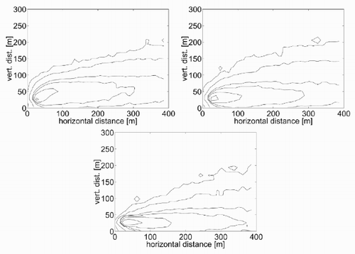
As was done for the basic test, an equivalence was sought between the results of figure 8 and a combination of the dispersion coefficients of the GPE. A choice of values for α, γ and δ that provide a satisfactory agreement for the ground concentration are listed in table 2. The corresponding concentration curves are shown in figure 9. These have been obtained with the GPE by imposing a plume rise height that varies with the downwind distance for the unstable and the neutral cases. For the unstable case, a linear-saturated relationship has been used and for the neutral case a straight linear relationship, whose features have been inferred from the plots in figure 8.

Figure 9. Concentration contour plots for the basic test with (a) Γ = − 0.3 K/m (b) Γ = − 0.01 K/m and (c) Γ = 0.5 K/m.

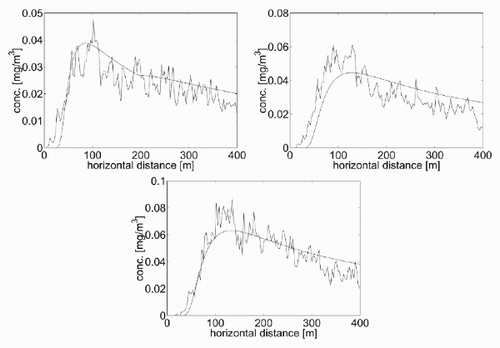
Table 2. Dispersion parameters as a function of Γ

Γ (K/m)	α	γ	δ
0.5	0.36	0.56	0.78
−0.01	0.35	0.6	0.79
−0.3	0.34	0.7	0.85

The ‘equivalent’ values found for α are rather constant, while γ and δ decrease as the stability increases. This dependence on the atmospheric stability is in substantial agreement with the most widely used semi-empirical relationships. In fact, α increases with increase in stability according to [12], but it is increasing–decreasing for [13, 14]. For the vertical dispersion σ_z , the value of the parameter γ is decreasing with increase in stability for all the correlations mentioned, while the parameter δ shows weaker variations, usually decreasing except in Turner's [14] correlation where it is increasing with increase in stability.

3.3 Effect of the buoyancy force

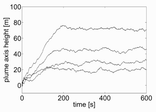
Another test was conceived to verify the capability of the model to represent different plume rise heights as a function of different emission temperatures. For the case shown in the previous section (figure 8), with an emission speed ν_e = 7 m/s and a temperature θ_e = θ_a = 295 K, the kinetic plume rise was around 20 m and there was no thermal plume rise. Now, if the emission temperature is increased to 300, 320, 350 and 400 K respectively, the plots in figure 10 are obtained. The increase in the thermal rise height is evident from figure 11. This shows the vertical distance of the plume centre from the source, as a function of the time from the beginning of the emission, for the various cases considered. Based on the curves in figure 11, it is also possible to evaluate the time after which the plume is steady. This varies in the range 100 – 200 s, increasing with increasing emission temperature.

Figure 10. Concentration contour plots for (a) θ _e = 300 K, (b) θe = 320 K, (c) θ _e = 350 K and θ _e = 400 K.

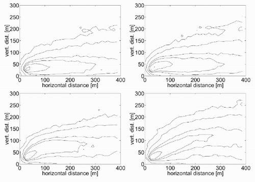
Figure 11. Rise in the axis of the plume as a function of the time from the emission start, for θ_e = 300, 320, 350 and 400 K from bottom to top.

In order to verify the reliability of the plume rise predictions shown in figure 10, the values obtained for the steady rise height are compared with those yielded by the most widely used empirical correlations, namely those in [15 –  17], as a function of temperature. Such a comparison is shown in figure 12. For all temperature levels considered, the values calculated with the lattice gas model are between those obtained from the CONCAWE [16] and the Briggs [15] correlations.

Figure 12. Plume rise height as calculated by the lattice gas model (□), by the Briggs [15] correlation (⋄), by the CONCAWE [16] correlation (*) and by the Holland [17] correlation (○).

4 Conclusions and future work

In this paper, a two-dimensional thermal lattice gas model for the gas dispersion in air has been presented. The model is of the HPP type, with four allowed velocities and a rest state. Air and pollutant particles have the same mass, and their distributions are represented by two distinct Boolean variables. The air particle distribution is randomly assigned at every time step in such a way as to meet a certain given air meteorological field. The pollutant particles obey various motion rules, in which an inherent randomness has been introduced.

The key to simulating buoyant plumes is the ability of the model to represent the gas temperature. Two different temperature definitions were considered; kinetic and statistical. The second was investigated in depth but, even though some advantages were recognizable, it had to be abandoned as unpractical. Together with the kinetic temperature, a rule to evaluate the buoyancy forces was added to the model.

The model provides predictions of the pollutant concentration which are qualitatively correct. All the main processes are well represented, including wind transport, turbulent diffusion, kinetic plume rise and thermal plume rise. Moreover, the quantitative predictions are in agreement with those obtained with a Gaussian plume model, in the steady-state limit. This point was verified with an equivalence found between the ground concentrations obtained with the lattice gas model and the Gaussian model, for a proper selection of the dispersion coefficients in the latter. In all the cases considered, the ‘equivalent’ dispersion coefficients are not in contrast with the values suggested by the most widely used empirical correlations.

Future work will include experimental validation of the model and comparison with direct numerical simulation tools in terms of computing time and resources. New rules representing chemical reactions and removal mechanisms are planned to be included in the next phase of model development. This will be done combining phenomenological information about these processes and the intrinsically probabilistic nature of the lattice gas model.

References

- Hardy , J , de Pazzis , O and Pomeau , Y . 1973 . Time evolution of a two-dimensional model system I: invariant states and time correlation functions . Journal of Mathematical Physics , 14 : 1746 – 1759 .
- Frisch , U , Hasslacher , B and Pomeau , Y . 1986 . Lattice gas automata for the Navier – Stokes equation . Physical Review Letters , 56 : 1505 – 1508 .
- Rothman D Zaleski S 1997 Lattice-Gas Cellular Automata Cambride Cambridge University Press
- Chopard B Droz M 1998 Cellular Automata Modeling of Physical Systems Cambridge Cambridge University Press
- Rivet J-P Boon J 2001 Lattice Gas hydrodynamics Cambridge Cambridge University Press
- Salcido A 1993 Lattice gas model for transport and dispersion phenomena of air pollutants In: P. Zannetti, C. Brebbia, J. Garcia Gardea and G. Ayala Milian (Eds) Air Pollution Southampton Computational Mechanics Publications
- Salcido A 1994 First evaluations of a lattice gas approach to air pollution modelling In J. Baldasano, C. Brebbia, H. Power and P. Zannetti (Eds) Air Pollution II 1 Southampton Computational Mechanics Publications
- Sciarretta A Cipollone R 2001 A lattice gas model for the evaluation of transport and diffusion parameters of stack emissions in air In: G. Latini and C. Brebbia (Eds) Air Pollution IX Southampton WIT Press
- Sciarretta A Cipollone R 2002 On the evaluation of pollutant gas dispersion around complex sources by means of a lattice gas model In: C. Brebbia and J. Martin-Duque (Eds) Air Pollution X Southampton WIT Press
- Burgess , C and Zaleski , S . 1987 . Buoyant mixtures of cellular automaton gases . Complex Systems , 1 : 31 – 57 .
- Chen , S , Chen , H , Doolen , G , Gutman , S and Lee , M . 1991 . A lattice gas model for thermohydrodynamics . Journal of Statistical Physics , 62 : 1121 – 1151 .
- Carpenter , S , Montgomery , T , Leavitt , J , Colpaugh , W and Thomas , F . 1971 . Principal plume dispersion models, TVA power plants . Journal of the Air Pollution Control Association , 21 : 491 – 495 .
- Pasquill , F . 1961 . The estimation of the dispersion of windborne material . Meteorology Magazine , 90, 33 – 49
- Turner D 1970 Workbook of Atmospheric Dispersion Estimates US Publication AP-26 Cincinnati Ohio National Air Pollution Control Administration
- Briggs G 1971 Some recent analyses of plume rise observations In: H. Englund and W. Berry (Eds) Proceedings of the 2nd Clean Air Congress New York Academic Pres 1029 1032
- Briggs G 1975 Plume rise predictions In: Lectures on Air Pollution and Environmental Impact Analyses Boston Massachusetts American Meteorological Society pp. 59 – 111
- Holland J 1953 A meteorological survey of the Oak Ridge area USAEC Report ORO-99 US Atomic Energy Commission Oak Ridge Tennessee USA