Modelling and reduction techniques for studies of integrated hybrid vehicle systems

Abstract

Models of integrated vehicle systems are essential for designing hybrid vehicles by means of simulation-based optimization. Given the complexity of hybrid vehicle systems, designing is a time consuming process that requires the evaluation of a large number of different design configurations. Modelling and simulation can significantly reduce the design time through efficient design evaluations and reduced number of prototypes built. This work presents the development and reduction of an integrated hybrid vehicle model composed of an engine, drivetrain, hydraulics and vehicle dynamics subsystems. For model development the bond graph formulation is used because it facilitates the integration of component/subsystem models in different energy domains, supports hierarchical modelling and allows straightforward manipulation of the model. The model is configured for a medium size military truck, and implemented in the 20SIM modelling and simulation environment. After developing the model, an energy-based model reduction methodology is applied in order to generate a reduced vehicle model that provides more design insight. The generated reduced system model for the hybrid truck (compared to the full model) produces almost identical predictions, has almost half the size and calculates the system response 2.5 times faster. This computationally efficient reduced model can be used for vehicle design studies to further reduce the development time.

Keywords:

• Bond graphs
• System dynamics
• Proper modelling
• Model reduction
• Hybrid vehicles

1 Introduction

Product development remains a costly and time consuming process despite the extensive use of modelling and simulation. In particular, the vehicle development process begins with a comprehensive analysis of the vehicle to determine the desired characteristics of its systems. It then proceeds with detailed design of systems, subsystems and components, and it concludes with the building and testing of prototypes. The latter may include engine, drivetrain, or vehicle subsystems and components, as well as the complete vehicle. In the case of hybrid powertrain vehicles, this process becomes even more cumbersome and time consuming due to system complexity and the increased number of subsystems and components. Development time and cost can be significantly reduced through systematic use of modelling and simulation. Modelling by means of time based simulations allows the testing of virtual vehicles for a variety of conditions, and designing of subsystems and components at the early development stages. In addition, a model-based simulation assists in quantifying parameters associated with subjective driver feel and overall drivability that are difficult to measure and yet very important for customer acceptance. However, the effectiveness of modelling and simulation is heavily dependent on the availability of comprehensive vehicle system, subsystem and component models that efficiently predict the variables of interest within the required accuracy.

Previous attempts to model the entire vehicle system have used a variety of approaches, differing in the fidelity of individual models as well as the methodologies used to integrate the various subsystems. Early attempts were based on empirically-based collections of look-up tables for the engine and drivetrain subsystems, and point mass vehicle dynamics models [1 –  3]. At that point, physical based models were difficult to develop and modify given the inadequate capabilities of modelling and simulation software environments.

Significant improvements in the integration methodology have since emerged, based on object-oriented graphical programming environments, such as EASY5 [4], AMESim [5], MATLAB/SIMULINK [6] and 20SIM [7]. These computer environments provide flexibility in connecting and interchanging models of subsystems, which greatly facilitates model assembly. As a result, engineers typically include any possible complexity or physical phenomena to generate system models capable of predicting every possible variable in the system regardless of relevance. This is common practice due to the lack of systematic approaches and metrics for determining the required physical phenomena to be included in the model for accurately predicting the variables of interest. In addition, computing resources are becoming faster and cheaper, alluring engineers into developing models that are even more complicated.

In an attempt to use the techniques and simulation environments mentioned above, Assanis et al. [8] developed a high fidelity vehicle simulation that was configured for a 6 × 6 tractor semi-trailer and integrated using the SIMULINK environment. In this work, emphasis was given on the high fidelity of all subsystems (e.g. crank-angle based engine model). The application of the complete vehicle simulation demonstrated the ability to predict the effect of engine system design changes on vehicle performance, as well as the complex interactions between the powertrain and the vehicle during highly transient manoeuvres. Additional development of such models created the Vehicle Engine Simulation (VESIM) modelling and simulation environment that also includes a library [9] with a variety of vehicle subsystem models. For efficient use of such complicated system models, special care must be given to model development in order to include only the necessary complexity.

A variety of algorithms have been developed to help automate the production of dynamic system models that are accurate yet simple (smaller in size). The most recent algorithm is a model reduction approach that uses an energy-based metric to produce proper models [10,11,12]. This approach can be applied to nonlinear as well as linear dynamic systems and considers the importance of energetic elements (inertial, compliant and resistive). The concept of a proper model was introduced by Wilson and Stein [13], who defined it as the model with the minimal set of physical parameters required to predict dominant system dynamics—along with an algorithm that deduces the appropriate system model complexity. Additional work on generating proper models has produced a series of algorithms for addressing different aspects of the model complexity problem [14,15,16]. Proper models are generally computationally more efficient, which is beneficial for design optimization where models are evaluated numerous times. In addition, they provide insight into the system for identifying the critical parameters and assisting the design process.

This work presents the development of a bond graph based integrated hybrid vehicle model of proper complexity, which is intended for design optimization. It is the objective of this work to present and establish the efficacy of the model reduction technique in a vehicle system modelling context. A military truck that belongs to the family of medium tactical vehicles (FMTV) is selected for the implementation of the proper modelling procedure. The vehicle consists of the engine, drivetrain and vehicle dynamics subsystems. In addition to the conventional powertrain a hydraulic propulsion and energy storage subsystem is included. A model that accurately predicts performance and fuel economy variables is necessary since the objective of the optimization is to improve fuel efficiency while maintaining some critical performance characteristics. Model reduction methodologies (energy-based modelling metric) are employed to identify the critical system parameters and reduce the model size. This reduced and computationally efficient model can then be used in a simulation-based design optimization, however, this next step is beyond the focus of this paper and it is described in the work of Filipi et al. [17].

The paper is organized as follows: the background on the energy-based model reduction metric and algorithm is presented in section 2. Next, the description of the military truck system and its model are given in section 3. Then, in section 4 the energy-based modelling metric is applied to the model to generate a reduced model. Finally, summary and conclusions are given in section 5.

2 Background—model reduction

The original work on energy-based metrics for model reduction [10,11] is briefly presented in order to provide the foundation for the contributions of this paper. The reduction procedure starts with a high-fidelity (full) model, and then based on an energy-based metric removes physical phenomena that are identified to be insignificant. To maintain the proper model properties the reduction proceeds by removing physical phenomena or/and quantities from the model (e.g. damper, mass, etc.). By operating on the physics of the model, the process yields a physically meaningful system model even after reduction. This approach is in contrast with model reduction techniques [18] used in the automatic control area, in which the states and parameters of the reduced models do not retain their physical significance. This reduces their usefulness for design analyses since the design parameters are not explicit in the reduced model.

The elimination of physical phenomena requires the identification of those elements that are not important and, therefore, do not contribute to the overall system behaviour. The power associated with each element in the system provides an indication of an element's contribution to the total behaviour of the system (at least as far as energy is concerned). An element with high power associated with it, stores (energy storage element) or absorbs (dissipative element) a sizeable portion of the power that is supplied into the system and, therefore, contributes significantly to the system behaviour. However, because power is time dependent, its use as a modelling metric would lead to varying instantaneous estimates of the elements' importance. In order to eliminate time dependency, the absolute value of power is integrated over time to a scalar metric:

where P(t) is the element power and T is the time window over which the activity is calculated. This scalar metric has units of energy and represents the amount of energy that flows in and out of the element over the time window T. The energy that flows in and out of an element is a measure of how active this element is (how much energy passes through it), and consequently the quantity in equation (1) is termed activity. It is assumed that the higher the activity, the higher the contribution of the element to the overall system behaviour. The activity is calculated for each energy element based on the system response.

The activity, as defined above, provides a measure of absolute importance of the elements. To provide a relative measure, the total activity (A _total) of the model, which represents the total amount of energy that flows in and out of the system over the period T, is defined. The total activity is then used to calculate a normalized metric called element activity index or just activity index. The activity index AI_i , as shown in equation (2), is calculated for each element in the model and represents the portion of the total system energy that is flowing through that element.

Here A_i is the activity of the ith element as given by equation (1) and k is the total number of energy elements in the model.

Note that for highly nonlinear systems the time response and quantities needed for calculating the activity index must be obtained numerically. First, numerical integration of the model produces the time response of the system states along with the necessary outputs (generalized effort and flow of all energy elements) for calculating the power. Then, the activities can be calculated using the expressions in equation (2).

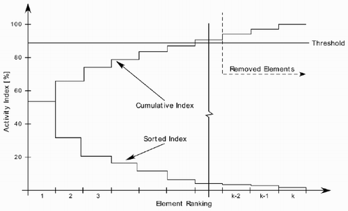
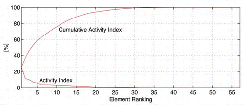
With the activity index defined as a relative metric for addressing element importance, the model order reduction algorithm (MORA) is constructed. The first step of MORA is to calculate the activity index for each element in the model for a given system excitation and initial conditions. Next, the activity indices are sorted to identify the elements with high activity (most important) and low activity (least important). With the activity indices sorted, the model reduction proceeds given some engineering specifications, which are defined by the modeller who then converts them into a threshold of the total activity (e.g. 99%) that he/she wants to include in the reduced model. This threshold defines the borderline between the retained and eliminated model elements. The elimination process is shown in figure 1 where the sorted activity indices are summed starting from the most important element until the specified threshold is reached. The element which, when included, increments the cumulative activity above the threshold, is the last element included in the reduced model. The elements that are above this threshold are eliminated from the model. The elimination of the low activity elements is done by removing these low activity elements from the model description.

Figure 1. Activity index sorting and element elimination.

2.1 Multi-dimensional activity

The activity metric as defined above is applicable to physical elements that are only allowed to move in one dimension. For example, systems with rotating shafts and translating masses connected together can be easily handled since the elements have a single degree of freedom (1-DOF). However, the activity as it is defined in equation (1) cannot be applied to rigid bodies moving in three-dimensional space with up to six degrees of freedom. For bodies moving in multi-dimensional space, we encounter the apparent problem that the scalar activity must somehow be calculated by force and velocity vectors. One way to resolve this is to assume that the activity for each DOF emanates from a different element even though there is only one physical element. This means that the power for each DOF is calculated using the corresponding component of force and velocity. Thus, for example, the mass of an object can be allowed to move in six directions (translational and rotational) but in a given scenario, only a subset of its DOFs might be important and have high activity. For the ith element of a system with p degrees of freedom, this can be written as:

where e _i ,f _i ∈ ℜ ^p are the generalized force and velocity vectors for the ith rigid body in the model. This approach for calculating the activity can produce a higher degree of reduction than that suggested by a cumulative activity for all degrees of freedom. This extension of the activity enables the implementation of MORA and the activity metric to many automotive systems.

3 Vehicle description and modelling

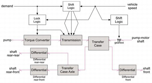
The vehicle is comprised of the engine, hybrid drivetrain and vehicle dynamics as shown in figure 2. In the conventional 6 × 6 drivetrain the engine drives the vehicle through the torque converter (TC), whose output shaft is then coupled to the automatic transmission (AT), which drives the transfer case (TrC) that equally splits the torque to the front and rear wheels. The front prop-shaft (PSF) delivers the torque to the front differential (DF). The other output of the transfer case, through the rear – front prop-shaft (PSRF), delivers power to the inter-axle transfer case (TrCA) that further splits the torque to the two rear axles. The first output of the inter-axle transfer case drives the rear – front differential (DRF) and the other the rear – rear differential (DRR) through the rear – rear prop-shaft (PSRR). Finally, the torque is delivered to the wheels through six half-shafts. For the purposes of this paper the vehicle dynamics are modelled using a pitch plane model since steering input is not considered. Therefore, left and right driveshafts of each axle are combined to deliver the driving torque to the wheel.

Figure 2. Schematic of the integrated vehicle system.

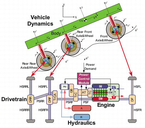
To provide the hybrid functionality, the drivetrain includes a hydraulic pump/motor (PM), accumulator (A) and reservoir (R) in addition to the conventional components. The pump/motor is connected to the transfer case after a fixed speed reduction provided by a gearbox (GB). The pump/motor is connected to the accumulator that stores a high pressure hydraulic fluid by means of compressed gas. On the other hand, the reservoir stores or supplies the hydraulic fluid used by the pump/motor. The operation of the hybrid drivetrain is controlled by the power management module, which determines the operating points of the engine, transmission, and the pump/motor based on the power demand and the available hydraulic fluid in the accumulator [17].

The model is developed using the 20SIM modelling environment that supports hierarchical modelling and allows the physical modelling of subsystems and components using the bond graph formulation [19,20]. This environment allows easy modification (addition or removal) of model complexity, which makes the reduction procedure using the activity metric a straightforward task. The model is developed with the intention of using the model reduction approach, therefore, all components and subsystems are allowed to have the maximum complexity, i.e. all physical phenomena are included in the model without considering their significance to the system behaviour. The system model complexity will be addressed with the energy-based metric.

At the top level of the model hierarchy (see figure 3), we have the engine, drivetrain, hydraulics and vehicle dynamics excited by the environment. One source of excitation is the driver who controls the vehicle speed through the gas and brake pedals. The driver can also control the vehicle heading through the steering wheel, however, the steering input is neglected and the vehicle is constrained to move only on the pitch plane. The driver is modelled as a controller that follows a driving cycle. The other excitation comes from the road, which is usually uneven and prescribes a vertical velocity to the tyres at the contact point. The road excitation is applied to all tyres (front, rear – front and rear – rear) as a function of their longitudinal position.

Figure 3. Top-level vehicle representation.

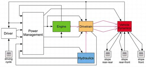
The vehicle operations are controlled by the power management strategy which is based on engineering intuition and simple analysis of component efficiencies [21]. The power management (see figure 3) first interprets the driver pedal signal as a power request and then according to the power request the operation is divided into two control modes: braking and normal. In the event of negative power request, braking mode is engaged to decelerate the vehicle. First the hydraulic pump is used to provide the required braking power and the remainder (if any) is provided by the friction brakes. If the power request is positive the normal mode is engaged, where the power is first supplied by the hydraulic motor and the remainder by the engine. In both cases the accumulator charge is allowed to vary from full to empty.

3.1 Engine

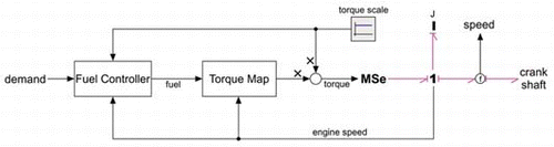
The engine model includes the inertial effects of all rotating parts that are lumped into an inertial element (J). The engine brake torque is produced from a look-up table as a function of engine speed and fuelling rate (see figure 4). This complexity of the engine torque calculation is sufficient for the purposes of this study where fuel economy is of interest. A linear torque scaling is also added to allow small engine changes for design studies. The engine power is managed by the fuel injection controller which provides the signal for the mass of fuel injected per cycle based on driver demand and engine speed.

Figure 4. Engine subsystem.

3.2 Drivetrain

The drivetrain provides the connection between the engine and the vehicle dynamics subsystems (see figure 5). The torque converter input shaft, on one end, and the three drive shafts, on the other end, are the connecting points for the engine and the vehicle dynamics models, respectively. The inputs are the engine speed and wheel rotational speeds and the outputs the torques to the wheels and load torque on the engine. Two additional inputs are the driver demand and vehicle speed, which are used by the shift and lock logic to determine the operation of the transmission and torque converter, respectively. Finally, a gearbox that is connected to the transfer case provides the connection for the hydraulic pump/motor.

Figure 5. Drivetrain subsystem.

The torque converter is the fluid clutch by which the engine is coupled to the transmission. The fluid coupling has characteristics of a gyrator since the pump and turbine torques are determined by the turbine and pump speeds. This gyrator is a nonlinear and non-power conserving element that accounts for energy losses due to fluid circulation. The pumping losses are modelled as a constant torque loss throughout the entire operating range. The transmission is modelled as a non-power conserving transformer that models gear efficiency and different gear ratios for seven gears. The speed reduction in each gear is assumed ideal, while the torque multiplication is reduced by a gear efficiency factor. The transmission fluid churning losses are also modelled. The differentials and transfer cases are modelled as non-power conserving transformers with ideal speed reduction but non-ideal torque multiplication based on a given gear efficiency. Finally the drivetrain inertia is included in the model.

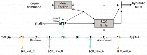
3.3 Hydraulics

The components in the hydraulics subsystem enable a more efficient use of the engine and regeneration during vehicle deceleration. The bond graph model of the hydraulics is depicted in figure 6. The central component is the pump/motor that is modelled with a non-power conserving modulated transformer (MTF) that accounts for volumetric and torque efficiencies. For the high pressure accumulator and low pressure reservoir a 2-port compliant (C) element is used, modelling both the fluid and heat transfer effects. The inert gas in the reservoir and accumulator is modelled as a real gas with a nonlinear constitutive law that accounts for pressure and temperature variations. There are two resistive elements (R_wall_A, R_wall_R) representing the energy exchange of the walls of the accumulator (or reservoir) with the environment (TaA, TaR). In addition, the fluid friction losses in the pipe connecting the pump/motor with the reservoir (and accumulator) are modelled with a nonlinear resistive element (R_pipe_R, R_pipe_A).

Figure 6. Components of hydraulics subsystem.

3.4 Vehicle dynamics

The vehicle dynamics subsystem considers the wheels, tyres, axles, suspensions and body of the vehicle. The vehicle is modelled as a collection of rigid bodies that are allowed to move on a plane subject to forces, moments and rigid constraints (figure 2). The truck body is modelled as a rigid body that is free to move horizontally and vertically, and to pitch. Three inertial elements are used to represent the dynamics in the three degrees of freedom. The kinematics are described in a body fixed frame (x,y) and represented by the nonlinear Euler equations. The body also includes three points for connecting the axles at fixed locations relative to the CG. Finally, aerodynamic drag is modelled by a resistive element that is quadratic in the forward vehicle velocity. The bond graph model of the vehicle dynamics is shown in figure 7.

Figure 7. Pitch plane dynamics subsystem.

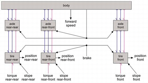
Each axle is modelled as a rigid body with its kinematics described in a body fixed frame (x_i ,y_i ). The axle is constrained by a rigid constraint to move on an axis that has its origin at the attachment point (P_i ) and it is perpendicular to the horizontal axis of the frame (x_i ,y_i ), where i = 1,2,3 represents the three axles. The axle is also constrained by the suspension, which is modelled as a linear spring and nonlinear shock absorber connected in parallel. The tyre model includes the wheel rotational dynamics and the interaction of the tyre with the road. Drive torques from the drivetrain are applied at the wheel hubs to accelerate the wheels and thus the vehicle. A simple brake model with viscous and Coulomb friction is included to generate the required torque for decelerating the vehicle. Tyre rolling resistance is added to the model as an additional source of energy loss. Tyre forces in the vertical direction are modelled as a linear spring and damper connected in parallel. The longitudinal traction force is linearly calculated from wheel slip. The tyre properties (traction force, rolling resistance and stiffness) are estimated from measured data of the actual tyre.

4 Activity analysis and model reduction

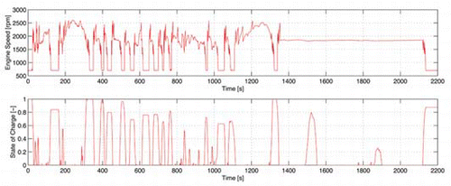
This model (or its reduced version) is intended for a design optimization study focusing on fuel economy improvement as the FMTV truck carries out a typical mission. This mission is described by a speed profile (driving cycle) that the truck must maintain as it drives over an uneven road profile. The cycle consists of city, highway and cross-country sections with prescribed forward velocity and road elevation. The driver model adjusts the throttle and brake signals in order for the vehicle to follow the prescribed speed profile. The response of the vehicle during this manoeuvre is shown in figure 8. Notice the fast transients of the engine as the vehicle accelerates/decelerates and shifts through the seven gears. The state of charge of the accumulator increases during decelerations and depletes during acceleration.

Figure 8. Integrated hybrid vehicle response.

The full model using the mission profiles can now be exercised to generate a reduced model using the activity metric. There are 57 energy elements in the model. The time window used to calculate the activity is the time needed for the vehicle to complete the cycle (2200s). The sorted element activity and cumulative activity indices for this manoeuvre are plotted in figure 9 and the numerical values tabulated in the appendix. Notice that the cumulative activity reaches approximately 90% after including the fifteen most important elements. The most important element (25.5% activity index) is the vehicle mass in the forward direction, while the least important element is the damping of the rear-rear tyre. The most active elements are related to the dynamics in the longitudinal direction and drivetrain energy losses, while the elements in the vertical and pitch directions are at the bottom of the list as the least important elements. Also, all activities of the reservoir elements are towards the bottom of the list, along with the activity of the accumulator pipe.

Figure 9. Integrated hybrid vehicle response.

4.1 Reduced model

The activity results can now be used to generate a reduced model. The element elimination starts with the least important element (vehicle\tyre_rear_front\B_tyre) and continues with elements of higher activity. Using a 99% threshold, MORA keeps only 30 elements of the full model, resulting in a reduced model that maintains 99.22% of the total activity and eliminates 27 energy elements. The eliminated elements include the suspension and tyre compliances, body moment of inertia and inertia of the axles in the vertical direction. In addition, the chamber compliance, friction and heat transfer resistance of the reservoir are eliminated. This means that the reservoir dynamics do not have a significant effect on the overall system response. Finally, MORA eliminates the resistive elements used to model the pipes' fluid friction, and the compliance and damping of the transmission shaft. The elimination of all these low activity elements produces a reduced model that has no pitch or vertical motion, which might be expected since we have a heavy vehicle riding on a relatively smooth surface. The reduced model only includes the body and axle masses in the longitudinal direction along with the aerodynamic drag. In addition, the wheel inertias, rolling resistances, brake losses and tyre slips are included. All drivetrain energy losses (pumping, churning and gear efficiencies) and engine inertia have high activity and, therefore, are included in the reduced model. The reservoir dynamics are eliminated and replaced with a constant pressure.

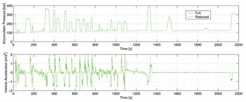
The reduced model is recompiled and used to predict the vehicle response for the same cycle. Figure 10 compares the accumulator pressure and vehicle acceleration as predicted by the reduced model versus the full model. The predictions from the two models are almost identical. The computational efficiency of the reduced model is improved by approximately 150% when using an Euler fixed-step integration scheme. Similar accuracy degradations are also observed for most system variables.

Figure 10. Comparison of the full and reduced model.

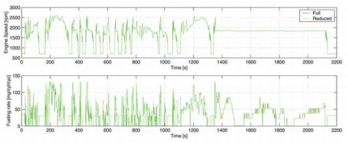
A comparison of variables associated with the engine performance is also performed to assess the accuracy of the reduced model over all vehicle components. Figure 11 shows the comparison of engine speed and fueling rate, which are required for accurate fuel economy predictions. The disagreement is minimal between the full and reduced models' predictions. The full model predicts 6.9404 kg fuel consumption for driving through the cycle, while the reduced model predicts 6.9326 kg. This amounts to 0.1128% loss in accuracy over the complete driving cycle, which is negligible compared to the improvements in model complexity and computational efficiency.

Figure 11. Comparison of the full and reduced model (engine).

5 Summary and conclusions

Development and reduction of an integrated hybrid vehicle system simulation in conjunction with a model reduction algorithm were presented in this paper. Such reduced models are beneficial to design optimization studies due to the physical insight, lower dimension design space and computational efficiency. A vehicle system model of an off-road truck belonging to the family of medium tactical vehicles (FMTV) is developed. The complete vehicle simulation was performed in 20SIM using a hierarchical modelling approach. The model complexity was addressed with an energy-based metric. By removing 27 out of the 57 elements a reduced model was produced which generated almost identical predictions as the full model. In addition, the computational efficiency of the reduced model was significantly improved (2.5 times faster).

While some outcomes of the model reduction procedure may seem intuitive to an expert in vehicles, they provide critical information to a modeller with less domain expertise. In addition, identifying the elements that contribute the most for a highly transient manoeuvre is in general not a trivial task. Generating the proper model with MORA provides critical information to the engineer. Perhaps the most readily assessable benefit is that the activity identifies the important parameters (elements) relative to a particular scenario. Thus, even if the model is not reformulated into reduced form, having a rank ordered list of the parameter importance directs the designer towards the design features that can produce the greatest effect on the system. Another benefit of ranking parameter importance is that the time and effort (cost) of obtaining model parameters can be reduced. A full model can be created with low precision parameter values. Then, upon learning which parameters are important, resources can be directed into obtaining higher precision values of the important parameters. Design optimization would also benefit from the knowledge of parameter importance by eliminating the need to perturb otherwise unimportant model parameters.

Another expected benefit from the elimination of energy storage elements from the model is computational efficiency. The computational efficiency of the reduced model is improved by both the reduction of the number of states and the increase of the integration time step due to elimination of high frequency dynamics from the model. However, the removal of inertial elements from a model may produce models that cannot be formulated into explicit equations using classical methods. Thus formulation of the reduced models remains an important research topic for not only computational efficiency but also for automating the generation of proper models as described previously. In addition, based on current knowledge, the designer would be required to eliminate elements systematically until the model complexity is just sufficient to produce the necessary accuracy. Presumably, an element elimination process could be automated, although this topic remains for future work.

Acknowledgments

The authors gratefully acknowledge the support of this work by the US Army Tank Automotive Command (ARC DAAE 07-94-Q-BAA3) through the Automotive Research Center (ARC) at the University of Michigan. The authors would also like to thank Bin Wu and Zoran Filipi for the development of the hydraulic subsystem models, Berrin Daran and Zoran Filipi for the development of the engine model, and Chan-Chiao Lin and Huei Peng for the design of the power management controller. In addition, Walter Budd and David Perry of Steward & Stevenson are recognized for providing critical information and data of the FMTV military truck. Finally, the contributions of Donald Szkubiel and Ron Chapp of the National Automotive Center are gratefully acknowledged.

APPENDIX: Activity analysis for the FMTV hybrid-hydraulic truck (elements in bold are eliminated)

Table

Ranking	Element	Activity [J]	Index [%]	Cumulative Index [%]
1	Vehicle\body\Mx	5.1715e+007	2.55133e+001	25.51334
2	Drivetrain\Transmission\B_churning	2.2549e+007	1.11244e+001	36.63779
3	Vehicle\body\R_aerodynamic	1.9681e+007	9.70950e+000	46.34729
4	Drivetrain\TC\T_pumping	1.3651e+007	6.73487e+000	53.08216
5	Hydraulics\Accumulator\Chamber	1.1445e+007	5.64611e+000	58.72826
6	Vehicle\tire_front\B_rolling	7.1795e+006	3.54197e+000	62.27023
7	Vehicle\tire_rear_front\B_rolling	7.1411e+006	3.52300e+000	65.79324
8	Vehicle\tire_rear_rear\B_rolling	7.1387e+006	3.52186e+000	69.31510
9	Hydraulics\Accumulator\R_wall	6.8556e+006	3.38218e+000	72.69728
10	Vehicle\axle_rear_rear\Mx	5.9891e+006	2.95470e+000	75.65198
11	Vehicle\axle_rear_front\Mx	5.9840e+006	2.95218e+000	78.60417
12	Drivetrain\Differential_front\losses	5.8319e+006	2.87714e+000	81.48131
13	Vehicle\axle_front\Mx	5.0733e+006	2.50289e+000	83.98420
14	Hydraulics\PM\losses	4.2780e+006	2.11053e+000	86.09473
15	Engine\I_engine	3.9787e+006	1.96285e+000	88.05759
16	Drivetrain\TC\FluidCoupling\losses	3.2093e+006	1.58330e+000	89.64089
17	Drivetrain\Differential_rear_front\losses	2.8998e+006	1.43061e+000	91.07151
18	Drivetrain\Differential_rear_rear\losses	2.8972e+006	1.42930e+000	92.50081
19	Drivetrain\Transmission\gear\losses	1.9456e+006	9.59874e−001	93.46068
20	Vehicle\tire_front\B_slip	1.4729e+006	7.26658e−001	94.18734
21	Drivetrain\Transmission\Inertia	1.4281e+006	7.04565e−001	94.89190
22	Vehicle\tire_front\B_brake	1.3934e+006	6.87403e−001	95.57931
23	Vehicle\tire_rear_front\B_brake	1.3750e+006	6.78325e−001	96.25763
24	Vehicle\tire_rear_rear\B_brake	1.3667e+006	6.74241e−001	96.93187
25	Vehicle\tire_front\J_wheel	1.0342e+006	5.10228e−001	97.44210
26	Vehicle\tire_rear_front\J_wheel	8.8095e+005	4.34613e−001	97.87671
27	Vehicle\tire_rear_rear\J_wheel	8.7611e+005	4.32226e−001	98.30894
28	Hydraulics\Accumulator\Chamber_friction	8.4240e+005	4.15593e−001	98.72453
29	Vehicle\tire_rear_front\B_slip	5.2304e+005	2.58039e−001	98.98257
30	Vehicle\tire_rear_rear\B_slip	5.2236e+005	2.57702e−001	99.24027
31	Vehicle\axle_front\C_susp	3.2080e+005	1.58263e−001	99.39854
32	Vehicle\tire_front\C_tire	2.3157e+005	1.14243e−001	99.51278
33	Hydraulics\Reservoir\Chamber	2.1439e+005	1.05766e−001	99.61855
34	Vehicle\axle_rear_rear\C_susp	1.2431e+005	6.13269e−002	99.67987
35	Vehicle\tire_rear_rear\C_tire	1.1806e+005	5.82436e−002	99.73812
36	Hydraulics\Reservoir\R_wall	1.1707e+005	5.77570e−002	99.79587
37	Hydraulics\R_pipe_accumulator	8.9364e+004	4.40873e−002	99.83996
38	Vehicle\tire_rear_front\C_tire	5.8731e+004	2.89744e−002	99.86894
39	Vehicle\body\My	5.8065e+004	2.86461e−002	99.89758
40	Vehicle\axle_rear_front\C_susp	5.8032e+004	2.86297e−002	99.92621
41	Hydraulics\R_pipe_reservoir	5.3618e+004	2.64524e−002	99.95266
42	Hydraulics\Reservoir\Chamber_friction	2.6737e+004	1.31907e−002	99.96585
43	Drivetrain\Transmission\R_shaft	1.9615e+004	9.67682e−003	99.97553
44	Vehicle\body\J	1.1748e+004	5.79579e−003	99.98133
45	Drivetrain\Transmission\C_shaft	1.0560e+004	5.20993e−003	99.98654
46	Vehicle\axle_front\My	8.4754e+003	4.18129e−003	99.99072
47	Vehicle\axle_rear_rear\My	7.3243e+003	3.61340e−003	99.99433
48	Vehicle\axle_rear_front\My	6.0449e+003	2.98221e−003	99.99731
49	Vehicle\axle_front\shock_absorber	2.9434e+003	1.45209e−003	99.99877
50	Vehicle\axle_rear_rear\shock_absorber	1.2690e+003	6.26078e−004	99.99939
51	Vehicle\axle_front\B_susp	5.2788e+002	2.60426e−004	99.99965
52	Vehicle\axle_rear_front\shock_absorber	2.5639e+002	1.26490e−004	99.99978
53	Vehicle\axle_rear_rear\B_susp	2.4427e+002	1.20510e−004	99.99990
54	Vehicle\tire_front\B_tire	6.9055e+001	3.40681e−005	99.99993
55	Vehicle\axle_rear_front\B_susp	6.1297e+001	3.02405e−005	99.99996
56	Vehicle\tire_rear_rear\B_tire	5.8547e+001	2.88836e−005	99.99999
57	Vehicle\tire_rear_front\B_tire	1.4129e+001	6.97063e−006	100.00000

References

- Haley PW Jurkat MP Brady PM 1979 NATO Reference Mobility Model—NRMM, Edition I, User's Guide, Volume I, Operational Modules Technical Report 12503 Warren MI US Army Tank-Automotive Research and Development Command
- Buck RE 1981 A Computer Program (HEVSIM) for Heavy Duty Vehicle Fuel Economy and Performance Simulation, Volume 2: Users' Manual US DOT Document #DOT-HS-805-911. Available at the Library, the University of Michigan Transportation Research Institution (UMTRI)
- Phillips , AW and Assanis , DN . 1989 . A PC-based vehicle powertrain simulation for fuel economy and performance studies—VPS . International Journal of Vehicle Design , 10 : 639 – 658 .
- Easy5 2000 Users' Manual Seattle WA The Boeing Company
- AMESim 2003 Reference Manual, Version 4.1 Roanne France IMAGINE S.A.
- MATLAB/SIMULINK 2002 User's Manual, Version 6.5 Natick MA The MathWorks Inc.
- 20SIM 2002 20SIM Pro Users' Manual, Version 3.3 Enschede The Netherlands The University of Twente—Controllab Products B.V. Available online at: http:\\www.20Sim.com
- Assanis D Bryzik W Chalhoub N Filipi Z Henein N Jung D Liu X Louca L Moskwa J Munns S Overholt J Papalambros P Riley S Rubin Z Sendur P Stein J Zhang G 1999 Integration and use of diesel engine, driveline and vehicle dynamics models for heavy duty truck simulation SAE paper 1999-01-0970
- Assanis DN Filipi ZS Gravante S Grohnke D Gui X Louca LS Rideout GD Stein JL Wang Y 2000 Validation and use of SIMULINK integrated, high fidelity, engine-in-vehicle simulation of the international class VI truck SAE Transactions Journal of Engines Warrendale PA Society of Automotive Engineers
- Louca LS Stein JL Hulbert GM Sprague JK 1997 Proper model generation: an energy-based methodology Proceedings of the 1997 International Conference on Bond Graph Modeling San Diego CA SCS
- Louca LS 1998 An energy-based model reduction methodology for automated modeling PhD thesis, The University of Michigan
- Louca LS Stein JL Hulbert GM 1998 A physical-based model reduction metric with an application to vehicle dynamics The 4th IFAC Nonlinear Control Systems Design Symposium (NOLCOS 98), Enschede, The Netherlands, July 1 – 3
- Wilson , BH and Stein , JL . 1995 . An algorithm for obtaining proper models of distributed and discrete systems . Transactions of the ASME: Journal of Dynamic Systems, Measurement and Control , 117 : 534 – 540 .
- Ferris JB Stein JL Bernitsas MM 1994 Development of proper models of hybrid systems Proceedings of the 1994 ASME International Mechanical Engineering Congress and Exposition—Dynamic Systems and Control Division, Symposium on Automated Modeling: Model Synthesis Algorithms New York NY ASME pp. 629 – 636
- Ferris JB Stein JL 1995 Development of proper models of hybrid systems: a bond graph formulation Proceedings of the 1995 International Conference on Bond Graph Modeling San Diego CA SCS pp. 43 – 48
- Walker , DG , Stein , JL and Ulsoy , AG . 2000 . An input-output criterion for linear model deduction . Transactions of the ASME: Journal of Dynamic Systems, Measurement and Control , 122 : 507 – 513 .
- Filipi ZS Louca LS Daran B Lin C-C Yildir U Wu B Kokkolaras M Assanis DN Peng H Papalambros PY Stein JL 2004 Combined optimization of design and power management of the hydraulic hybrid propulsion system for the 6 × 6 medium truck International Journal of Heavy Vehicle Systems (Special Issue on Advances in Ground Vehicle Simulation) 11 3 372 402
- Moore , BC . 1981 . Principal component analysis in linear systems: controllability, observability, and model reduction . IEEE Transactions on Automatic Control , AC-26/1 : 17 – 32 .
- Karnopp DC Margolis DL Rosenberg RC 1990 System Dynamics: A Unified Approach New York NY Wiley-Interscience
- Brown FT 2001 Engineering System Dynamics: A Unified Graph-Centered Approach New York NY Marcel Dekker
- Wu B Lin C-C Filipi Z Peng H Assanis D 2002 Optimization of power management strategies for a hydraulic hybrid medium truck Proceedings of the 6th International Symposium on Advanced Vehicle Control AVEC ‘02, Hiroshima, Japan, September 9 – 13 pp. 559 – 564