Structured SM identification of vehicle vertical dynamics

Abstract

In this paper the problem of identifying discrete time nonlinear systems in regression form from finite and noise corrupted measurements is considered. According to the specifications about identification accuracy that may be needed, a good exploration of the regressor domain of interest has to be ensured by the experimental conditions. This problem becomes very significant for growing dimension of the regressor space, leading very easily to computational complexity problems and to inaccurate identified models. These difficulties are significantly reduced if, using information about the physical structure of the system to be identified, this can be decomposed into interacting subsystems. Using this structural information, the high-dimensional identification problem may be reduced to the identification of lower dimensional subsystems and to the estimation of their interactions. Typical cases considered in the literature are Hammerstein, Wiener and Lur'e systems, but the paper shows that the approach can be extended to more complex structures composed of many subsystems and with nonlinear dynamic blocks, using as an example the identification of a half-car model for vehicle vertical dynamics, where nonlinear suspensions and tyres are considered. Assuming that the road profile is given and that front and rear vertical accelerations are measured, an experimental setup easily realizable in actual experiments on real cars, the half-car model, is decomposed as a generalized Lur'e system, consisting of a linear MIMO system, connected in a feedback form with the two nonlinear dynamic systems through non-measured signals. An iterative identification scheme is proposed, which makes use of a set membership method for the identification of the nonlinear dynamic blocks. This method does not require assumptions on the functional form of the involved nonlinearities, thus circumventing the identification accuracy problems that may be generated by considering approximate functional forms. The numerical results demonstrate the effectiveness of the proposed approach.

Keywords:

• Structured identification
• Set membership identification
• Semi-active suspensions
• Ride comfort models

1. Introduction

Consider a discrete nonlinear dynamic system with m inputs

and q outputs

of the form:

Suppose that the functions

are not known, but a set of noise corrupted measurements of

and

k = 1, …, q, t = 1,2,…T is available, and it is of interest to identify the system, i.e. to find estimates

of

, possibly giving ‘small’ identification error.

According to the specifications about identification accuracy that may be needed, a good exploration of the regressor domain of interest has to be ensured by the set of measured regressors

. However, exciting a system in order to obtain such a good exploration is still an open problem in nonlinear systems identification theory. This problem becomes very significant for growing dimension of the regressor space, leading very easily to computational complexity problems and to inaccurate identified models. These difficulties can be significantly reduced if, using information about the physical structure of the system to be identified, this can be decomposed into interacting subsystems. Using this structural information, the high-dimensional identification problem may be reduced to the identification of lower dimensional subsystems and to the estimation of their interactions. Typical cases considered in the literature are Hammerstein, Wiener and Lur'e systems, consisting of two subsystems, a linear dynamic one and the other nonlinear static, connected in cascade or feedback form. In practical applications more complex structures may be needed, e.g. composed of many subsystems and with nonlinear dynamic blocks.

In this paper we propose an approach able to deal with more complex structures. A key feature is that the nonlinear subsystems may also be dynamic and are not supposed to have a given parametric form. Indeed, a method recently developed in [1,2], not requiring assumptions on the functional form of involved regression functions, but assuming only some information on their regularity, is used for nonlinear subsystems identification. In this way the complexity/accuracy problems [3,4] posed by the proper choice of the suitable parametrization of the nonlinear subsystems are circumvented.

Since the decomposition structure is highly dependent on the specific system to be studied, we consider here as a paradigmatic example the problem of identifying a half-car model for vehicle vertical dynamics. Identification is performed on simulated data obtained by a half-car model where the chassis, the engine and the wheels are simulated as rigid bodies, and the suspensions and the tyres are simulated as static nonlinearities.

The paper is organized as follows. In section 2 the nonlinear set membership identification method is summarized. In section 3 unstructured identification of vehicle vertical dynamics is performed. In section 4 structured identification of vehicle vertical dynamics is performed. In section 5 some concluding remarks are made.

2. Nonlinear SM identification

In this section the nonlinear SM identification method developed in [1,2] is summarized.

Consider the system (1) for the case k = 1 and omit the index k for simplicity. Suppose that a set of noise corrupted data

and

generated by (1) is available. Then:

where the term d_t accounts for the fact that y_{t  + 1} and w_t are not exactly known.

The aim is to derive an estimate

of f _o from available measurements

, i.e.

. The operator φ, called the identification algorithm, should be chosen to give small (possibly minimal) error

, where ||·|| _p is the standard L _p norm

, p∈[1,∞),

ess-sup _w∈W |f(w)| and W is a bounded subset of

. This error is not known, since from available data it is only known that

, the set of all f that can have generated the data. This set, even in case of exact measurements, is unbounded, since the mapping generating data from given f is not injective. Then, whatever algorithm φ is chosen, no information on the identification error can be derived, unless some assumptions are made on the function f_o and the noise d. The typical approach in the literature is to assume a finitely parametrized functional form for f_o (linear, bilinear, neural network, etc.) and statistical models on the noise [3,4,5,6]. In the present SM approach, different and somewhat weaker assumptions are taken, not requiring the selection of a functional form for f_o , but related to its rate of variation. Moreover, the noise sequence D_T  = [d ₁,d ₂, … d_T ] is only supposed to be bounded.

Prior assumptions on f_o :

Prior assumptions on noise:

Here, f′(w) denotes the gradient of f(w) and

is the Euclidean norm.

A key role in this set membership framework is played by the feasible systems set, often called the ‘unfalsified systems set’, i.e. the set of all systems consistent with prior information and measured data.

Definition 1. Feasible systems set

The feasible systems set FSS _T is:

The feasible systems set FSS _T summarizes all the information on the mechanism generating the data that is available up to time T. If prior assumptions are ‘true’, then f_o  ∈ FSS _T , an important property for evaluating the accuracy of inferences that can be done on the system.

As typical in any identification theory, the problem of checking the validity of prior assumptions arises. The only thing that can actually be done is to check if prior assumptions are invalidated by data, determining if no system exists consistent with data and assumptions, i.e. if FSS _T is empty. Indeed the fact that the priors are consistent with the present data, i.e. FSS _T  ≠ Ø, does not exclude the possibility that they may not be consistent with future data. However, it is usual to introduce the concept of prior assumption validation as follows.

Definition 2. Validation of prior assumptions

Prior assumptions are considered validated if:

Necessary and sufficient condition for checking the validity of assumptions are now given. Let us define the functions:

where

and

.

Theorem 1.

	, is a necessary condition for prior assumptions to be validated.
	, is a sufficient condition for prior assumptions to be validated.

Proof. See [1].

Note that there is essentially no ‘gap’ between the necessary and sufficient conditions, since the condition

, t = 1,2,…,T, is sufficient for any δ > 0 arbitrarily small and necessary for δ = 0. In this paper it is assumed that the sufficient condition holds. If not, values of the constants appearing in the assumptions on the function f_o and on the noise d_t are accordingly changed. The validation Theorem 1 can be used for assessing the values of such constants such that the sufficient condition holds (see [7,8]).

An identification algorithm φ is an operator mapping all available information about the function f_o , noise d, data

until time T, summarized by FSS _T , into an estimate

of the function f_o :

The related L_p error is:

This error cannot be exactly computed, since it is only known that f_o ∈ FSS _T , but its tightest bound is given by

. This motivates the following definition of the identification error, often indicated as worst-case or guaranteed error.

Definition 3. Identification error

The identification error of

is:

Looking for algorithms that minimize the identification error leads to the following optimality concepts.

Definition 4. Optimal algorithm

An algorithm φ* is called optimal if:

The quantity r_I , called the radius of information, gives the minimal identification error that can be guaranteed by any estimate based on the available information up to time T.

An optimal algorithm is provided by the following result. Let the function f_c be defined as:

where f _l (w) and f _u (w) are defined in (4).

Theorem 2.

For any L _p (W) norm, with p ∈ [1,∞]:

(i) The identification algorithm φ_c (FSS _T ) = f_c is optimal;

(ii)

.

Proof. See [2].

So far a global bound on

over all W is assumed. However, a local approach can be taken in order to obtain improvements in identification accuracy, e.g. by assuming different bounds γ _k on suitable partitions W _k of W. This is similar to what is done in identification of the piecewise linear model, where partitions W _k W _k are looked for, over which f _o (w) can be considered approximately linear, i.e.

const., ∀w ∈ W _k (see, e.g. [9] and [10]). However, finding such partitions may not be an easy task. A very simple alternative approach allowing the use of local assumptions on f _o is based on the evaluation of a function f _a approximating f _o (using any desired method) and on the application of the method described in this paper to the residue function

using the set of values Δy ^t + 1  =

i = 1,2,…, T. Then, the estimate:

is used, where

is the central estimate of f _Δ(w) obtained from data Δy ^t + 1 , t = 1,2,…,T.

Assuming a global bound

on the residue function f _Δ implies the local bound

for the function f _o .

If the function f _a is chosen as the estimate within a parametric model family, the present ‘local’ approach allows us to investigate the effects of neglected dynamics and of possible trapping in local minima during the parameter estimation phase. In fact, if f _a and

have comparable identification accuracy, a confirmation is obtained that the chosen model family is sufficiently rich to accurately approximate f _o and that a ‘good’ minimum, if not the global one, is reached. On the other hand, the model

may give accuracy improvements over model f _o in case the chosen model family is not sufficiently rich and/or the minimization process got stuck in a local minimum.

3. Unstructured identification of vehicle vertical dynamics

Models of vehicle vertical dynamics are very important tools in the automotive field, especially in view of the increasing diffusion of controlled suspension systems [11,12]. Indeed, accurate models may allow efficient tuning of control algorithms in a computer simulation environment, thus significantly reducing the expensive in-vehicle tuning effort.

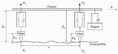
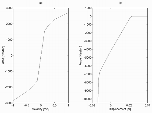
Structured and unstructured identifications are performed on simulated data obtained by the half-car model shown in figure 1. The chassis, the engine and the wheels are simulated as rigid bodies. Static nonlinearities have been considered for suspensions and tyres. In particular, the force – velocity characteristic of the suspensions and the force – displacement characteristic of tyres are reported in figure 2.

Figure 1. The half-car model.

Figure 2. (a) The force – velocity characteristic of suspensions. (b) The force – displacement characteristic of tyres.

The half-car model, called for short the ‘true system’, has been implemented in Simulink in order to obtain data simulating a possible experimental setup, characterized by type of exciting input, experiment length, variables to be measured and accuracy of sensors. The vehicle is assumed to travel at a constant speed V = 60 km/h. The main variables describing the model are:

1.	p rf and p rr: front and rear road profiles;
2.	a cf and a cr: front and rear chassis vertical accelerations;
3.	p cf and p cr: front and rear chassis vertical positions;
4.	p wf and p wr: front and rear wheels vertical positions;
5.	F cf and F cr: forces applied to chassis by front and rear suspensions;
6.	F wf and F wr: forces applied to front and rear wheels by tyres.

It is considered that the road profile p _rf (t) is known, that

and that the variables a _cf (t), a _cr (t), can be measured with a precision of 5%.

Two data sets have been generated from ‘true system’ simulation, by recording the values of p _rf, p _rr, a _cf and a _cr with a sampling time of τ = 1/512 sec. The first set, called the estimation set, is composed of 10 240 data values and corresponds to 20 seconds of ‘true system’ simulation on a random road profile with amplitude ⩽ 2.6 cm. The estimation data set, corrupted by a uniformly distributed noise of relative amplitude 5%, has been used for model identification. The second set, called the validation set, composed of 2049 data values, corresponding to 4 seconds of ‘true’ data not used for estimation, has been used to test the simulation accuracy of identified models.

The experimental setup simulated here has been chosen because it is not too complex to be realized in an actual experiment on a real car. A richer setup could give better identification results. For example, as will be clear in the sequel, if the forces F _cf and F _cr are also measured, the identification procedure becomes much simpler and more accurate. However, accurately measuring such forces requires more complex instrumentation of the car.

Discrete time models, relating front chassis accelerations to the road profile at the sampling times, have been identified from the estimation data set. In particular, an overall nonlinear model, indicated as NSMU (nonlinear set membership unstructured), not using information on the system structure, has been identified using the set membership approach presented in [1,13].

The model is of the form (1) with q = 2, m = 2,

,

, and

. The choice of n_y, n ₁, n ₂ has been made by considering that the system has order 8. Models with values of n_y, n ₁, n ₂ between 5 and 10 have been identified and the best one has been chosen, having n_y  = 8, n ₁ = 4, n ₂ = 4.

The simulation results of such a model have been tested on the validation data set. Because of space limitations, results related to the front acceleration are reported, but those related to the rear acceleration are similar.

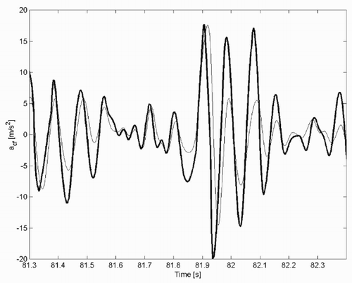
In figure 3 ‘true’ data and those obtained by the identified NSMU model are reported. The root mean square simulation error on the validation data set is reported in table 1 below.

Table 1: Root mean squared front chassis acceleration errors on the validation data set.

Model	NSMU	NNU	NSMS1	NSMS2	NSMS3
RMSE	3.27	3.37	2.56	2.41	2.05

Figure 3. Front chassis accelerations: ‘true’ (bold line); NSMU model (thin line).

The simulation accuracy appears to be not quite satisfactory. In order to check that this is not due to poor performance of the identification method, alternative models have been identified using the neural network toolbox of Matlab. Several two-layer neural networks with sigmoidal basis functions and with number of neuron ranging from 3 to 20 have been trained on the estimation set and the best one, having six neurons, has been chosen and is called NNU. The simulation results on the validation data set reported in table 1 suggest that by using only the available data without further information on the system, no more accurate models could be obtained. A structured identification approach is then explored.

4. Structured identification of vehicle vertical dynamics

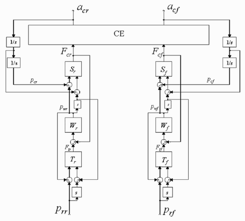
Considering its physical structure, the half-car model can be represented by the block diagram of figure 4.

Figure 4. Block diagram of half-car model.

The block CE represents the behaviour of the chassis and engine. Since for usual road profiles the chassis pitch angles are small (< 5 – 6 degrees), this block can be considered linear. The blocks S _f and S _r represent the behaviour of the front and rear suspension dampers and springs. These blocks are the main sources of nonlinearities in the system, mainly due to the significant nonlinearities of the dampers, see figure 2(a). The blocks W _f and W _r represent the inertial behaviour of the front and rear wheels and unsprung masses. These blocks are linear. The blocks T _f and T _r represent the behaviour of the front and rear tyres. These blocks are also nonlinear, see figure 2(b).

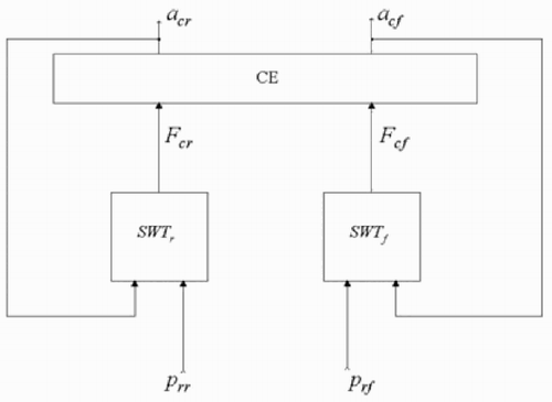
The block diagram of figure 4 can be represented in a more compact form by the block diagram of figure 5, which is then used for a structured identification procedure.

Figure 5. Generalized Lur'e form of half-car model.

In this form, the half-car model is represented as a generalized Lur'e system, consisting of the linear MIMO system CE, connected in a feedback form with the two nonlinear dynamic systems SWT_f and SWT_r, representing the overall behaviour of the front and rear suspensions, wheels and tyres. Note that here we have the same situation occurring in the identification of Hammerstein, Wiener or Lur'e systems: only input and output are measured (in the present case p _rf, p _rr, a _cf and a _cr), while the connecting variables are not measured (in the present case F _cf and F _cr). A widely used method for dealing with this problem is based on an iterative scheme (see, e.g. [14,15,16,17]), which in the present case can be adapted as follows:

1.	Assume an initial model for system CE.
2.	Evaluate the forces F cf and F cr required to generate measured accelerations a cf and a cr through the current model of CE.
3.	Identify nonlinear models of SWTf and SWTr using as output data the forces F cf and F cr estimated at step and as input data the measured accelerations a cf and a cr and known road profiles p rf and p ir.
4.	Identify a new model of CE using as output data the measured accelerations a cf and a cr and as input data the forces F cf and F cr simulated by means of the nonlinear models of SWTf and SWTr identified at step 3.
5.	If the simulation accuracy of the structured model NSMS, obtained by using, in the scheme of figure 5, the models of SWTf and SWTr identified at step and of CE identified at step 4, is not satisfactory, return to step 2.

The initial model required at step 1 has been obtained from the laws of motion, assuming the chassis and engine as a unique rigid body, leading to a 2 × 2 transfer matrix with constant elements. Indeed, the ‘true’ 2 × 2 transfer matrix has elements which are transfer functions of order 4, see figure 6 where the Bode plots of elements (1,1) of these transfer matrices are reported. This undermodelling is intentionally introduced, in order to verify the effects of errors in the initial guess of the iterative procedure. It can be noted that this initial model error is relevant, giving large errors (= 100%) in the initial estimates of the forces F _cf and F _cr, see figure 7.

Figure 6. Bode plots of CE(1,1): ‘true’ (bold line); initial model (dashed line); model at iteration 3 (thin line).

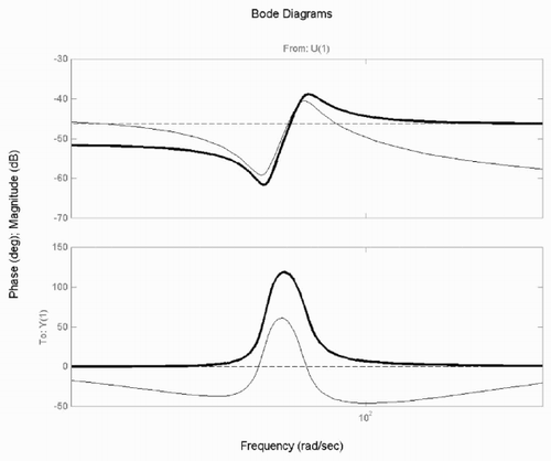
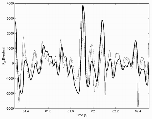
Figure 7. Forces applied to chassis from suspensions: ‘true’ (bold line); initial estimate (dashed line); estimate at iteration 3 (thin line).

In step 3, discrete time nonlinear models of SWT_r and SWT_r are identified using the set membership approach presented in [1,13]. The models are of the form (1) with q = 1, m = 2,

,

, and

, where * stands for ‘f’ or ‘r’. The choice of n_y, n ₁, n ₂ has been made by considering that the systems SWT_f and SWT_r have order 2. Models with values of n_y, n ₁, n ₂ between 1 and 6 have been identified and the best one has been chosen, having n_y  = 2, n ₁ = 2.

In step 4, the models of CE have been obtained by identifying linear output error models by means of the Matlab Identification Toolbox, with inputs F _cf, F _cf and outputs a _cf, a _cr.

The results derived by the NSMS _j models identified at iterations j = 1,2,3 are then compared with ‘true’ data on the testing data set.

In figure 6 the Bode plots of the elements (1,1) of the ‘true’ transfer matrix CE and transfer matrices identified at the first and third iterations are reported.

In figure 7 the ‘true’ forces applied to the chassis by the front suspension and those estimated at the first and third iteration are shown.

In figure 8 the ‘true’ front acceleration and those estimated by NSMS₁ and NSMS₃ are shown.

Figure 8. Front chassis accelerations: ‘true’ (bold line); NSMS₁ model (dashed line); NSMS₃ model (thin line).

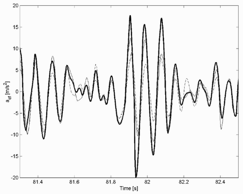
In table 1 the root mean square simulation errors between ‘true’ and estimated front accelerations are reported. It can be noted that after three iterations the estimates of the transfer matrix CE and of the forces F _c* are significantly improved, reflected in significant improvements of identification accuracy evaluated by chassis accelerations errors. Finally, it can be noted that the RMSE errors provided by the unstructured models NNU and NSMU are about 60% greater than the RMSE error provided by the structured model NSMS₃.

5. Conclusions

Block-oriented or structured identification is one of the most common approaches used in the literature to face the computational complexity and accuracy problems in identification of complex nonlinear systems. Most of the literature considers decompositions with two subsystems, a linear dynamic and a nonlinear static subsystem. Moreover, the nonlinear static subsystem is supposed to have a given parametric function form (polynomial, piecewise polynomial, etc.).

In this paper we have proposed an approach able to deal with more complex structures. A key feature is that the nonlinear subsystems may also be dynamic and are not supposed to have a given parametric form. In this way the complexity/accuracy problems posed by the proper choice of suitable parametrization of the nonlinear subsystems are circumvented.

The effectiveness of the proposed approach is tested on a simulated half-car model for vehicle vertical dynamics, where nonlinear suspensions and tyres are considered. The simulated experimental conditions allow a decomposition as a generalized Lur'e system, consisting of a linear MIMO system, connected in a feedback form with two nonlinear dynamic systems. The structured models identified by the proposed method in a few iterations reduce significantly the simulation errors, largely improving over unstructured models and reaching quite satisfactory identification accuracy.

Acknowledgements

This research was supported in part by Ministero dell'Università e della Ricerca Scientifica e Tecnologica under the Project ‘Robustness techniques for control of uncertain systems’ and by GM-FIAT World Wide Purchasing Italia under the Project ‘Modeling of vehicle vertical accelerations’.

References

- Milanese M C. Novara C 2002 Set membership estimation of nonlinear regressions IFAC 2002 Barcelona Spain
- Milanese M C. Novara C 2003 Optimality in SM identification of nonlinear systems Proc. 13th IFAC Symposium on System Identification SYSID 2003 Rotterdam The Netherlands
- Haber , R and Unbehauen , H . 1990 . Structure identification of nonlinear dynamic systems – a survey on input/output approaches . Automatica , 26 : 651 – 677 .
- Sjöberg , J , Zhang , Q , Ljung , L , Benveniste , A , Delyon , B , Glorennec , P , Hjalmarsson , H and A. Juditsky , A . 1995 . Nonlinear black-box modeling in system identification: a unified overview . Automatica , 31 : 1691 – 1723 .
- Narendra , KS and Mukhopadhyay , S . 1997 . Neural networks for system identification . Sysid 97 , vol. 2 : pp. 763 – 770
- Isermann , R , Ernst , S and Nelles , O . 1997 . Identification with dynamic neural networks – architectures, comparisons, applications . Sysid 97 , vol. 3 : pp. 997 – 1022
- Novara C Milanese M 2001 Set Membership prediction of nonlinear time series Proc. 40th IEEE Conference on Decision and Control Orlando FL pp. 2131 – 2136
- Milanese M C. Novara C 2002 Nonlinear Set Membership prediction of river flow Proc. 41st IEEE Conference on Decision and Control Las Vegas Nevada
- Sontag , ED . 1981 . Nonlinear regulation, The piecewise linear approach . IEEE Trans. Automatic Control , 26 : 346 – 357 .
- Ferrari-Trecate G Muselli M Liberati D Morari M 2001 A clustering technique for the identification of piecewise affine systems In: A. Sangiovanni-Vincentelli and M.D. Di Benedetto (Eds) Hybrid Systems: Computation and Control Lecture Notes in Computer Science Berlin Springer-Verlag
- Krtolica , R and Hrovat , D . 1992 . Optimal active suspension control based on a half-car model: An analytical solution . IEEE Transaction on Automatic Control , 37 : 2238 – 2243 .
- Lu , J and DePoyster , M . 2002 . Multiobjective optimal suspension control to achieve integrated ride and handling perfomance . IEEE Transactions on Control Systems Technology , 10 : 807 – 821 .
- Novara C Milanese M 2000 Set Membership identification of nonlinear systems Proc. 39th IEEE Conference on Decision and Control Sydney Australia pp. 2831 – 2836
- Narendra , KS and Gallman , PG . 1966 . An iterative method for the identification of nonlinear systems using a Hammerstein model . IEEE Transaction on Automatic Control , 11 : 546 – 550 .
- Stoica , P . 1981 . On the convergence of an iterative algorithm used for Hammerstein system identification . IEEE Transaction on Automatic Control , 26 : 967 – 969 .
- Vörös , J . 1999 . Iterative algorithm for parameter identification of Hammerstein systems with two-segment nonlinearities . IEEE Transaction on Automatic Control , 44 : 967 – 969 .
- Wemhoff E Packard A Poolla K 1999 On the identification of nonlinear maps in a general interconnected system American Control Conference San Diego CA