Equilibrium set investigation using bicausality

Abstract

The introduction of the bicausality concept in the bond graph language has allowed new analytical methodologies, for instance in the context of model inversion, mechatronic system sizing and control. The bicausality concept is here applied for solving the equilibrium state of a mechatronic system. We propose a new method, which permits us to determine the size of the equilibrium set and the algebraic system to be solved. The proposed method is applied to linear systems in a first step, and a generalization is also given for some non-linear systems. Several examples are included in order to explain the method.

Keywords:

• Bond graph
• Bicausality
• Equilibrium
• Sizing
• Design
• Inverse problem

1 Introduction

Since the introduction of the principles of bond graphs, the interest in bond graphs has been shown to be the basis of complex and pluridisciplinary system modelling [1]. Research was also carried out to develop a system analysis using the graphic support of bond graph and the concept of causality. The causal loop order studied by Van Dixhorn [2] sheds light on the organization of equations in models. Karnopp [3], Breedveld [4], Dauphin-tanguy [5] and Cornet [6] introduced several procedures based on causal assignment to determine system dynamic properties and to assist the synthesis of control law. Recently, the bicausality concept introduced implicitly by Cornet and Lorenz [7] and more formally by Gawthrop [8,9], has initiated a new philosophy with regard to the bond graph model. The essential concept of bicausality is that the causal stroke can be split into two bicausal half-strokes; this concept has established new rules for causal assignment and made a new range of problems accessible. This principle has been successfully applied in design or sizing problems by Fotsu-Ngwompo [10,11] and in control synthesis by Gawthrop [12,13]. Causality has to be regarded as a graphical principle to check the physical validity and the mathematical complexity of a given problem. The concept of bicausality also permits the searching of what information is required to solve a problem and which mathematical properties are needed to retain the physical meaning for the solution. A major contribution of the bicausality concept is that it defines reliable resources means to study inverse problems.

Bicausal half-strokes indicate the fixed or known variables of the bond and therefore determine the way to solve the modelled problem. This approach is also consistent for normal causality where it is still possible to split the causal stroke in one effort and one flow half causal stroke. All these aspects, including the bicausality assignment and the bicausal elements, are part of the bond graph modelling package MS1 (Lorenz Simulation) [14,15,16], which has been developed in close cooperation with the authors for all aspects related to bicausality.

In this paper, the bicausality concepts are used to solve the problem of the existence and the determination of the equilibrium set of a system using a bond graph model. If we consider a system defined by its state model (1), where x is the state vector and u the input vector, the resolution of the equilibrium consists in solving the algebraic system (2):

Using the bond graph representation of a system, P. Breedveld [17] has proposed a procedure to determine the equilibrium state. At steady state, the energy stored in each storage element is constant, that is to say the values of the energy variables are constant and the values of their derivatives are zero. On the bond graph, the efforts (respectively the flow) of the I-elements (respectively the C-elements) have then to be zero, and Breedveld proposes replacing the I-elements by null effort sources and the C-elements by null flow sources.

There are three limitations using this approach. First, the condition of use of this procedure is that all the storage elements in the bond graph in integral causality have to be in integral causality. This means that there is no static dependency between energy storage. Second, after replacing the storage elements by the corresponding sources, a causal conflict may appear and the proposed procedure is no longer valid. Finally, if the causality assignment is possible, all the input values have to be known in order to determine the steady state. This means that the values of all sources and modulation signals have to be fixed, although this is rarely the case in practice.

Due to these important limitations, the purpose of this paper is to complete the procedure proposed by Breedveld and to show the advantages of using the bicausality for the resolution of the equilibrium set.

2 Nature of the steady state problem

As previously introduced, Breedveld's procedure proposes replacing all the I-elements by null effort sources and the C-elements by null flow sources. In this step if there is no causal conflict and if all the inputs (sources and modulation signals) are known, it is possible to determine the output values (detectors) at steady state.

First of all, we can remark that this procedure leads to a single solution, if it exists, corresponding to calculation of the steady state values of the energy storage elements being given the input values. But usually, it is interesting to find the dimension of the solution because it shows how many state variables and input variables have to be fixed in order to determine an equilibrium point. The set of known variables, or more generally the variables for which values can be fixed, is strongly dependent on the problem that has to be solved. However the problem may be to determine the steady state from given input values; it is also very common in the control or design context to search the value of a source or an input, which allows a specific steady state to be reached. In this last case, the problem can be interpreted as an inverse problem [18,19].

Let us consider a time invariant linear system represented by its state equation (3). In this case, the equilibrium set is defined by equation (4). An equilibrium point is then a solution of a linear algebraic system, whose unknowns are (x_e ,u_e ). From linear algebra analysis, the dimension q of the solution is defined by equation (5). Therefore, the values of the q variables in a subset have to be fixed in order to completely define a specific equilibrium point. It is generally not possible to choose any set E _obj and the right decision has to be done in order to find the equilibrium state.

Although the rank of

is generally not calculated, one may remark that this rank is always greater than or equal to the rank of the state matrix A (equation 6). This interesting property shows that dynamic dependencies in the system may lead to a greater dimension of the equilibrium set (equation 7), and also that the input location may only decrease this dimension by decoupling the equations of the state matrix.

Our purpose is here to study the equilibrium problem using bond graph modelling. The previous remarks show that an important aspect of this problem is to determine the dynamically dependent state or energy variable in the system [20]. We will show that this can be graphically achieved using causality and bicausality. As this problem has to be put in the general context of system control, this work includes also models with bond graph and signal subsystems.

According to the assumptions in Breedveld's procedure, a single equilibrium point does not exist if there is a causal conflict when changing storage elements into their corresponding zero source. In fact, these causal conflicts show that there are dynamic dependent storage elements in the system, and therefore the dimension of the equilibrium set is greater than or equal to the number of inputs in the system. An infinity of equilibrium points exists and the solution is a space, whose directions are a subset of E _obj ⊂ (x∪u). As the rank of the system state matrix is determined from the number of storage elements staying in integral causality on the bond graph in derivative causality [20], we can conclude that the existence of an equilibrium point can be determined by solely applying derivative causality to the bond graph without changing any elements. If any storage element stays in integral causality in the bond graph in derivative causality, there is a dynamic dependency and the rank of the model state matrix is no longer equal to its order. This last case is not developed in this work; however the consequences are briefly examined in section 5.

Example

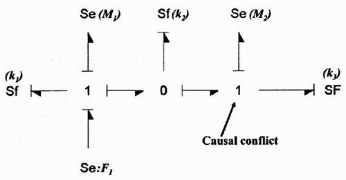
The mass – spring system (figure 1) shows a simple case in which it is not possible to conclude using Breedveld's procedure (figure 3). The dimension and the order of the model are 5, as there are the five storage elements in integral causality in the bond graph in integral causality. The rank of the system state matrix is only 4, as there is one storage element remaining in integral causality in the bond graph in derivative causality (figure 2). Using equation (7), we can conclude that the dimension of the equilibrium set is less than or equal to one.

Figure 1. Schema of a mass – spring system.

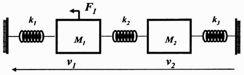
Figure 2. Bond graph in derivative causality.

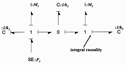
Figure 3. Breedveld's procedure.

3 Using bicausality to introduce constraints

Bicausality allows splitting the causal stroke into two parts, each one being related to either flow or effort power variable. Using this facility, it is possible to define three types of sources and three types of detectors:

1.	SeDf: effort source – flow detector (equivalent to classical effort source);
2.	SfDe: flow source – effort detector (equivalent to classical flow source);
3.	SeSf: effort and flow source;
4.	DeSf0: effort detector – zero flow source (equivalent to the classical effort detector);
5.	DfSe0: flow detector – zero effort source (equivalent to the classical flow detector);
6.	DeDf: effort and flow detector.

Apart from the double source and detector, which constitute new elements, the other ones are equivalent to classical bond graph elements with a slight distinction, which consists in giving a meaning to all the power variables on the bond. From a mathematical point of view, all the detected variables correspond to all the variables, which have to be evaluated; they are the outputs or unknowns of the mathematical problem. Respectively, all the source variables represent all the variables, which have to be imposed; they constitute the inputs or known values of the mathematical problem.

According to the previous remark, these elements can be efficiently used to clarify the procedure enabling the research of the equilibrium set. Whereas Breedveld's procedure only determines the equilibrium point, given the source element values, bicausality permits us to use any variable in the set E _obj as input of the problem. If the dimension of the equilibrium set is greater than or equal to one, double source elements can be used to force specific steady states for one or more energy variables, instead of imposing input or source values. An I-element will then be replaced by a double source, where first, the effort is set to zero in order to impose the steady state condition to the element, and second, the flow has the value corresponding to the desired steady state. The C-elements may be replaced similarly but in this case the flow of the double source element is set to zero, and the effort has the value corresponding to the desired steady state.

The use of the bicausality concept and inverse problem methodology will enable correct sets of variables to be chosen. Section 6 will detail this procedure.

4 Control variables

For control purposes, some auxiliary signal integrations may be required. They have to be carefully defined at the modelling stage as they may introduce dependency with energy storage elements. We assume in the rest of the paper that these auxiliary integrations define p independent equations. The auxiliary signal integrations have to be connected to either junctions, or detectors, or other signals in the bond graph. In the state model, they then introduce p equations (8):

The steady state condition imposes relation (9), which may be introduced in the bond graph by splitting the integrators and by introducing the relation corresponding to the steady state at the input and output of the integration. In order to impose these conditions on the bond graph, we propose first to replace the integrator input by a zero signal source and also to reverse the corresponding signal bond, and second, to replace the integrator output by a signal source corresponding to the steady state value. If the integrator input is directly connected to a detector or a junction, zero double sources have to be used. There are two reasons for this replacement. On the one hand, one of the power variables of the zero double source element has to impose the steady state condition similarly to energy storage elements. On the other hand, it is also necessary to force the other power variable to zero because this new source is not a physical energy source but a constraint, and also because this variable has no meaning and should not have an effect on the system steady state equations.

Another consequence of the use of a double source is that one of the power sources has to be changed into a double detector DeDf in order to keep the dimension of the input vector and then the dimension of the equilibrium set. The choice of the source to change into a double detector will be discussed in section 6.

When all the integrators have been replaced to introduce the steady state conditions, each remaining algebraic relation in the signal part must be considered (9). For each relation, one of the variables has to be chosen as a new output of the relation, whereas the other ones will stay as inputs. This choice must be made according to the problem to be solved and also according to the bond graph obtained at the end of the steady state procedure. In some non-linear cases, the algebraic equation (9) is implicitly defined and a more complex procedure would be required to obtain explicit equations.

Example

Figure 4 illustrates the proportional position control of a pendulum actuated by a DC motor. On the physical part of the bond graph (figure 5), it can be determined that the rank of the system state matrix is 2 as there is no storage element in integral causality in the bond graph in derivative causality. Including the signal part, there are three equations (two energy state variable +  one signal integration) and four variables (i, ω, θ, θ₀) corresponding to three state variables and one input signal variable. A single equilibrium point can be calculated when one of these variables is given. In other words, the equilibrium set dimension is one.

Figure 4. Proportional position control of a pendulum actuated by a DC motor.

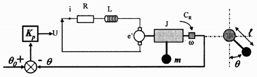
Figure 5. Bond graph in integral causality.

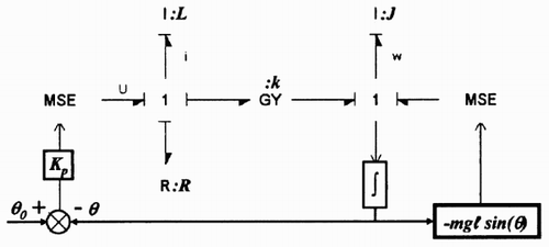
First, the integrator input is replaced by a zero double source as it is directly connected to a 1-junction. The procedure correctly introduces the fact that the equilibrium corresponds to a constant angular position, which also implies a zero angular velocity. The consequence is that bicausality can no longer be used to force a specific value for the energy variable related to the I-element (p2) at steady state as a conflict of causality would occur.

The integrator output is then replaced by a signal source corresponding to the equilibrium angular position θ _e . In order to solve the algebraic relation (10), two of the related variables (U_e ,θ_{0 e} , θ _e ) have to be supplied:

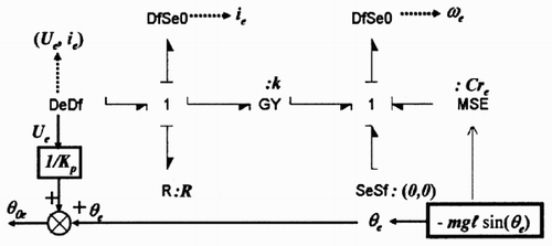
One of the energy sources has now to be replaced by a double detector to keep the dimension of the input vector. If the source corresponding to U_e is chosen, it becomes a DeDf. Assuming that θ _e is known, the remaining energy storage elements can be replaced by the corresponding zero source-detector: the I-elements (p1,p2) are changed into DfSe0. The implicit relation (10) becomes an explicit relation and θ_{0 e} can be computed using equation (11). The obtained bond graph (figure 6) permits us to compute the angular velocity ω _e and the current i_e at steady state according to equation (12):

In this previous example, several calculation schemes could have been developed. Using the same procedure, (i_e , θ _e , ω _e ) can be computed knowing the control input θ_{0 e} ; this corresponds to a control problem. Moreover, instead of propagating the bicausality towards the effort source U, the other effort source C _γ may also be used. In fact, any variables in the subset (i_e , θ _e , θ_{0 e} ) can be chosen as the known variable and used to compute the other ones. Note that the steady state value for ω _e is fixed to zero (as obviously expected) because of the zero double source. The procedure is then consistent as it not possible to freely set its value. Trying to force a specific equilibrium state for ω _e will require this element to be replaced by a double source element, and consequently will lead to a causal conflict as two bicausal bonds will be imposed on the same junction.

Figure 6. Determining the equilibrium point, given θ _e .

5 Dependent energy variables

Dependency between energy variable may occur and has to be carefully examined when a specific steady state is searched.

5.1 Statically dependent energy variable.

During the modelling stage, dependent energy variables may be defined in the system and they are associated to storage elements in derivative causality on the bond graph in integral causality [20]. The cause of the derivative causality may be related to an energy source imposing the co-energy variable behaviour, but more generally it corresponds to a dependency between energy variables. A zero order causal loop will indicate the dependent variables and it is usually possible to choose any of the energy variables of the causal loop as the dependent variable.

One possibility is then to simplify the bond graph by modifying its structure and determining the equivalent energy storage. However, the previous solution is not absolutely necessary and especially when the steady state is researched. At steady state, any dependent energy storage introduces a null power in the system because its power variable is computed from the derivative of the chosen independent energy variable. A dependent I-element (respectively, dependent C-element) is then replaced by a zero effort source – flow detector DfSe0 (respectively a zero flow sources – effort detector DeSf0). An important remark is that these dependent elements should not be used as steady state constraints and be replaced by double sources because of the dependency on another energy variable.

5.2 Causal conflict in the equilibrium bond graph.

When the bond graph in derivative causality presents n_D storage elements, which stay in integral causality, the rank of the model state matrix is no longer equal to its order n = n_I [20]. This case corresponds to causal conflict in Breedveld's procedure. These conflicts may occur due to causal paths with sources or other storage elements. From a mathematical point of view, it corresponds to the existence of n_D null eigenvalues. It indicates that there are r=n_i−n_d dynamically independent variables, and that the model order is r. It is then necessary to suppress n_D equations in order to obtain a full rank model.

When the causal conflicts occur due a causal path with a source element, it can result in a non-equilibrium case if the equilibrium condition of the storage element cannot be verified. The values of the considered sources have to be either equal to zero or set to zero through modulation or modulated elements such as a transformer or gyrator. However the dynamic dependency is broken by the source location, and the rank of the matrix

is greater than the rank of the state matrix A.

Some storage elements may stay in integral causality due to dependency with other storage elements and not from source location. This indicates that these elements have independent initial conditions but that there is an algebraic relationship between the states (energy variables) of the elements. It implies that the steady state will be related to the initial conditions of the concerned storage elements, that is the initially stored energy in the causal loop. Contrary to the previous case, the dependency between equations in the state matrix will remain and the rank of the matrix

will not increase. To determine the equilibrium, all the causal loops with other storage elements have to be identified. Within these storage elements, only one can introduce the steady state using the adequate source (Se for C-elements and Sf for I-elements); the other ones are left in derivative causality. It is then possible to solve the equilibrium problem.

6 Imposing the steady state condition

The dimension of the equilibrium set indicates the number of variables that must be known in order to define a specific equilibrium point. According to the problem to be solved, the set of known variables may vary. The problem can be either to determine the inputs to obtain specific values for the outputs, or to define the energetic state reached by the system, given the inputs, or any combination of the previous case. This approach is very close to a design problem as defined by Fotsu-Ngwompo et al. [18,19]. In the general case, it is not possible to choose any subset of state variables and inputs as known variables. Firstly, the number of variables to impose is limited by the dimension of the equilibrium set, and secondly, some combination of imposed variables may introduce causal conflicts. Indeed, if the considered storage element is related to causal conflicts due to sources or to zero order causal loops in the bond graph in derivative causality, a specific procedure has to be used. The concepts of bicausality and input – output causal path are here useful to determine if the chosen subset is adequate to solve the steady state problem.

If the power variable of an energy source or a modulation variable is chosen as a known variable, there is no consequence on the bond graph. But if it is a co-energy variable, two conditions are introduced at the same place on the bond graph: the equilibrium condition and the steady state value. Although it is possible to introduce this constraint on the bond graph using an adequate double source (SeSf0 for a C-element and a SfSe0 for an I-element), this requires us also to introduce double detectors. Either energy sources, or a modulated elements (in fact, the control variable) may be used as the new outputs. But any choice is not adequate. A causal path between the imposed variable (the steady state of the co-energy variable) and the input to compute have to exist in the bond graph in integral causality. Any input variable which is linked by a causal path with the considered co-energy variable in the bond graph in integral causality can be chosen.

Considering the search for a specific equilibrium point, the number of equilibrium states that may be imposed to energy storage elements is limited by the dimension of the equilibrium set. This case naturally corresponds to an inverse method as some inputs of the system become outputs. In order to verify if the choice of a subset of imposed steady states leads to a solvable system of equations, a set of disjoint causal paths has to exist in the bond graph in integral causality between the imposed co-energy variables and the outputs to compute. The causal loops which are related to storage elements that stay in integral causality in the bond graph in derivative causality (as indicated in section 6) have also to be taken into account.

If a set of disjoint causal paths does exist, the bicausality can be assigned from the different double sources SeSf towards the double detectors DeDf. The new system to solve can be obtained if it is still possible to complete the causality with the assignment of derivative causalities to the rest of the bond graph. Otherwise it shows that the choice is not adequate as causality conflicts will take place.

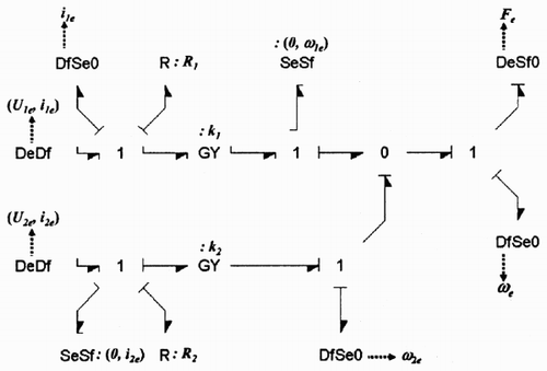
Example

Let us consider the bond graph (figure 8) representing a load driven by two DC-motors coupled by a differential described on figure 7. As one storage element is in derivative causality in the bond graph in integral causality (figure 8), the order of the model is 5. Applying derivative causality, we show that the rank of the system state matrix is equal to the model order, that is 5. The dimension of the equilibrium set is then 2, and consequently, two variables have to be known to define a specific equilibrium point.

Figure 7. Schema of the physical system.

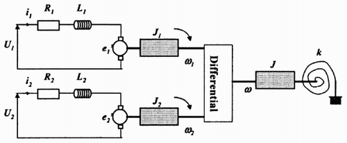
Figure 8. Bond graph in integral causality with the zero order causal loops and a set of disjoint causal paths.

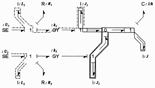
If the problem is to compute the values of the sources in order to obtain a specific equilibrium state of the system, only two energy storage elements can impose their steady state on the system. Figure 8 shows a set of disjoint causal paths from the two effort sources towards the co-energy variables of a couple of energy storage. Some other sets of disjoint causal paths can be identified on the bond graph, but for example, it is not possible to choose as imposed state the couple constituted by the C-element and the I-element (ω), or by the I-elements (ω) and the I-element (ω₁). In these two cases the causal paths are not disjoint and causal conflict would occur if they were used.

The equilibrium bond graph (figure 9) is deduced from the proposed procedure by substituting the chosen storage elements by double sources SeSf imposing the steady state and the equilibrium condition, and propagating the bicausality towards the effort sources, which are replaced by double detectors DeDf. The other storage elements are replaced by the adequate zero source-detector and finally, the causality is assigned to the rest of the bond graph. The obtained bond graph gives the calculation scheme (equation 13), which expresses the equilibrium point as a function of the imposed steady state values.

Figure 9. Equilibrium bond graph.

7 Equilibrium procedure

From the previous sections, a global procedure can be defined to determine first the dimension of the equilibrium set, and second a specific equilibrium point.

1.	Determine the order n of the model, which is equal to the number nI of storage elements in integral causality in the bond graph in integral causality.
2.	Impose the equilibrium conditions to the p integrators in the signal part and assign the derivative causality to the bond graph.
3.	Determine the rank r of the system state matrix, which is equal to the difference between nI and the number nD of storage elements that stay in integral causality in the bond graph in derivative causality.
4.	Identify the causal paths between the storage elements in integral causality and sources in the bond graph in derivative causality. For each element, check if there is a modulated transformer or gyrator on one of the paths or if it is possible to control the value of the sources. Otherwise the equilibrium cannot exist. Mark the chosen loops.
5.	Identify the causal loops between the storage elements in integral causality in the bond graph in derivative causality and other storage elements. Choose the dependent storage element within the concerned elements of the loops and mark the loops.
6.	From points 3, 4 and 5 determine the rank of the matrix [A:B] and the dimension of the equilibrium set.
7.	According to the researched equilibrium point, define the storage elements, for which the steady state will be known.
8.	On the bond graph in integral causality, determine a set of disjoint input – output causal paths, where the inputs are the power variables of the controllable sources and/or the modulation signals, and the outputs are the co-energy variables to be imposed in steady state and/or the power variables corresponding to signal integration and imposing constraints at the junctions. The marked causal paths and causal loops corresponding to steps 4 and 5 have to be taken into account.
9.	If there is at least one set of disjoint input – output causal paths, replace the storage elements where the steady states and/or constraints are imposed by double sources SeSf, and the chosen sources by double detectors DeDf. Propagate the bicausality between the SeSf and the DeDf or the modulated elements. Introduce the resolution of the dependent storage elements corresponding to steps 4 and 5. Assign a derivative causality to the rest of the bond graph.
10.	If there is a causal conflict, try another set of disjoint input – output paths. If there is no other set of disjoint input – output paths, the subset of imposed variables is not adequate for solving the equilibrium.
11.	On the bond graph in derivative causality, replace the storage elements in derivative causality by the adequate zero source-detector (DeSF0 for C-elements and DFSe0 for I-elements) and assign causality to the rest of the bond graph. Solve the system using the orientation of the characteristic relations defined by the causal assignment.

8 Conclusion

Based on causal analysis and the use of the bicausality concepts, this paper should complete Breedveld's approach for solving equilibrium problems. The existence and the dimension of the equilibrium set are only determined from a causal analysis of the bond graph. Then a complete procedure is proposed and allows a specific equilibrium point to be determined, given either input signals, or energy source value, or specific steady states of energy storage elements. The adequacy of the chosen subset of known variables can be easily checked before computing the equilibrium point. The developments introduced in this paper can naturally be extended to systems with multiport elements [21] and with non-linear elements. In these cases, the possible causal and bicausal assignments must be checked carefully before applying the procedure.

The search for equilibrium points is usually considered as a straightforward problem as it is only the starting point before linearizing the model. Nevertheless, it can be useful to have a correct value for an equilibrium point to define good initial conditions for complex simulations. The study of the steady state is also generally the first step of a system design, and for this purpose, the proposed procedure may show many advantages. Actually, the sizing of any parameter can be considered as a variable and introduced as a signal input in the bond graph. Determining a specific equilibrium point can then be used to compute this parameter. From our point of view, it is in this context that the proposed procedure will show many advantages over other methods.

References

- Karnopp DC Rosenberg RC 1968 Analysis and Simulation of Multiport Systems – The Bond Graph Approach to Physical Systems Dynamics Cambridge MIT Press
- van Dixhoorn J Evans F (Eds) 1974 Physical Structure in Systems Theory: Network Approaches to Engineering and Economics London Academic Press
- Karnopp DC Margolis DL Rosenberg RC 2000 Systems Dynamics: Modeling and Simulation of Mechatronic Systems New York John Wiley
- Breedveld PC van Dixhorn J 1989 Bond graphs in science and engineering IMACS Annals of Computing and Applied Mathematics 3 Modeling and Simulation of Systems Basel Baltzer pp. 5 – 6
- Dauphin-tanguy G et al. 1999 Modélisation des systèmes physiques par bond graphs: Ouvrage Collectif Paris Editions Masson
- Cornet A Lorenz F 1989 Equation ordering using bond graph causality analysis IMACS Annals of Computing and Applied Mathematics 3 Modeling and Simulation of Systems Basel Baltzer pp. 55 – 58
- Cornet A Lorenz F 1997 Equation ordering using bond graph causality analysis 12th IMACS World Congress 1 Paris pp. 43 – 46
- Gawthrop PJ 1995, Bicausal bond graphs Proceedings of ICGBM'95 Las Vegas pp. 83 – 88
- Gawthrop , PJ . 2000 . Physical interpretation of inverse dynamics using bicausal bond graphs . Journal of The Franklin Institute , 337 : 743 – 769 .
- Fotsu-Ngwompo , R , Scavarda , S and Thomasset , D . 1996 . Inversion of linear time invariant SISO systems modeled by bond graph . Journal of the Franklin Institute , 333B : 157 – 174 .
- Fotsu-Ngwompo , R and Scavarda , S . 1999 . Dimensioning problems in system design using bicausal bond graphs . Simulation Practice and Theory , 7 : 577 – 587 .
- Gawthrop PJ 1997 Control system configuration: Inversion and bicausal bond graphs Proceedings of ICGBM'97 Phoenix pp. 97 – 102
- Gawthrop PJ Ballance DJ Dauphin-Tanguy G 1999, Controllability indicators from bond graphs Proceedings of ICGBM'99 San Francisco pp. 101 – 107
- Lorenz F Erhard P 1997 MS1: A multi-formalism modeling and simulation environment Proceedings of ICGBM'97 Phoenix pp. 192 – 196
- Lorenz F 1999 New features in MS1 Proceedings of ICGBM'99 San Francisco pp. 169 – 174
- MS1: Lorenz Simulation Available online at: http://www.lorsim.be
- Breedveld PC 1984 Physical systems theory in terms of bond graphs PhD thesis, Twente University of Technology Enschede, The Netherlands
- Fotsu-Ngwompo , R , Scavarda , S and Thomasset , D . 2001 . Physical model-based inversion in control systems design using bond graph representation. Part 1: Theory . Proceedings of the IMECHE Part I, Journal of Systems and Control Engineering , 215 : 95 – 103 .
- Fotsu-Ngwompo , R , Scavarda , S and Thomasset , D . 2001 . Physical model-based inversion in control systems design using bond graph representation. Part 2: Applications . Proceedings of the IMECHE Part I, Journal of Systems and Control Engineering , 215 : 105 – 112 .
- Karnopp , DC . 1979 . On the order of a physical system model . Journal of Dynamic Systems, Measurements, and Control , 101 : 185 – 186 .
- Bideaux E Martin de Argenta D Marquis-Favre W Scavarda S 2001 Applying causality and bicausality to multi-port elements in bond graphs International Conference on Bond Graph Modeling, Proceedings of ICGBM'01 18 – 25 January, 2001, Orlando, Florida, CD-ROM