Results to aid applications of ellipsoidal state bounds

Abstract

Results to assist in the application of the ellipsoidal bounds provided by standard state-bounding algorithms are presented. They include derived bounds on scalar state-dependent quantities and the state values which determine them, tests of intersection and inclusion of ellipsoids, measures of how much an ellipsoid may be changed without altering its inclusion in another, and an ellipsoidal inner bound for the set reachable in the worst case from an ellipsoidal set by ellipsoidally bounded forcing, in a linear system. Approximations are suggested for the most computationally demanding result. Ways in which these results might be employed in aerospace interception problems are discussed to illustrate their utility.

Keywords:

• State estimation
• State bounding
• Ellipsoids
• Reachability analysis
• Aerospace control

1. Introduction

Recursive updating of bounds on the state of a dynamical system is a long-established alternative to probabilistic state estimation [1 –  8]. At each observation instant, the error in a vector of observed output variables is assumed to have known bounds, so bounds on the outputs at that instant can be inferred from the observations. They are translated, via the observation equation, into bounds on the current state. The discrete-time state equation also imposes time-updated bounds on the state, by combining bounds on the state at the previous sampling instant and specified bounds on the effects of forcing inputs since then. The feasible set of state values consistent with all observations up to the present is found by combining the time-updated bounds and the new observation-derived bounds.

As new observations add state bounds, the feasible set becomes inconveniently complicated. A simpler outer-bounding approximation is therefore usually updated, the most popular choice being an ellipsoid. The ellipsoidal bound

on the state at observation instant k has centre

, axes along the eigenvectors of P _k and half-axis lengths equal to the square roots of the eigenvalues. The updating algorithm for

and P _k aims to make the ellipsoid as tight as possible, usually by minimizing tr P _k , |P _k | or a combination [3]. The recursive ellipsoid-updating algorithms are algebraically quite similar to the Kalman filter, and there is an obvious analogy between

and P _k in equation (1) and the mean and covariance updated by the Kalman filter. The analogy is closer if the mean and covariance are those of a Gaussian posterior probability density function (pdf) of state, as then the confidence ellipsoid defined by

and P _k is a direct analogue of the state-bounding ellipsoid. Bounding can (but need not) be regarded as a component part of probabilistic state estimation if the bounds are regarded as defining the finite support of a state pdf.

Batch algorithms for ellipsoidal state bounding also exist [7]. They usually produce much tighter bounds than do the recursive algorithms but are, of course, less suited to real-time use. The results in this paper are applicable to ellipsoids generated by either batch or recursive algorithms.

Ellipsoidal state bounds can be used for two purposes for which they are better suited than probabilistic state estimation yet which have received less attention than they deserve. The first is to produce bounds on practically significant, scalar functions of state. Bounds on certain variables may be needed for control or decision support when the state coordinate system does not give them directly, being chosen instead to give a simple model. For example, Cartesian coordinates are often convenient for modelling motion, while polar variables may be preferred for guidance or collision avoidance. Section 2 shows that bounds on scalar functions of state can be found from ellipsoidal state bounds in several important cases. By contrast, the mean and covariance of a nonlinear function of state cannot generally be derived from the estimated state mean and covariance, and are not readily found even if the state pdf is Gaussian.

The second potential use of ellipsoidal state bounds is to check whether the future state, subject to uncertainty, can meet some desired condition. Examples are checking whether the future state can definitely be brought into a specified desirable region, true if its feasible set is contained in that region; checking if two objects can be made to meet or to miss in future, as in interception or collision avoidance; and unequivocal fault detection when the feasible set is outside the ‘no fault’ region. It is fairly straightforward to detect whether two ellipsoids intersect or one contains the other. If they do not intersect, the smallest change (translation, expansion or contraction) required to make one ellipsoid intersect or contain the other can also be found readily. This may show, for example, what action is necessary for the whole range of uncertain predicted position of a target to be reachable, ensuring interception. Similarly, when one set contains the other, it is easy to find the largest expansion or contraction factor for which that remains true.

The next section gives results for bounds on state-derived scalar quantities. Section 3 considers the intersection and inclusion of ellipsoids, and ellipsoidal reachable sets. Section 4 illustrates their utility by outlining applications in aerospace interception.

2. Bounds on scalar functions of state

2.1 Linear functions

The extremes of a scalar, linear function

over the ellipsoid

are at the points of tangency of the supporting hyperplanes of

normal to φ. The points are readily found by the Lagrange multiplier method:

so the extremes of f are

. As each extreme point is the intersection of a hyperplane and the strictly convex ellipsoid, it is unique.

By use of equation (3), the usual ellipsoid-updating state-bounding algorithms [1 –  6] can be modified to make the state bounds as tight as possible in any nominated direction (e.g. that of a particular crucial state variable). However, this is at the cost of bound looseness in other directions, so a better idea is to find the feasible set as the intersection of a number of ellipsoids, each tight in a different direction. A refinement would be first to find the minimum-volume bounding ellipsoid by the standard algorithm, then to update the ellipsoids tightest in the axis directions of that ellipsoid.

2.2 Ratio of two state variables

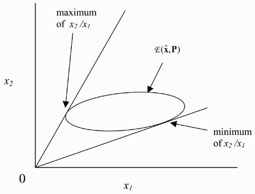
This case covers derivation of bounds on azimuth or elevation θ from joint bounds on Cartesian position components and their derivatives. For instance, for a target bounded by

, with (x ₁, x ₂), the Cartesian position coordinates of the target in the horizontal plane with respect to an observer at the origin, the azimuth extremes are defined by the extremes of x ₂/x ₁ over

, as sketched in figure 1. Another example is discrimination between target types, by comparing bounds on the image intensities of the target in two spectral bands, measured by a multispectral infrared sensor, with bounds on their ratio for different types of target.

Figure 1. Extremes of x ₂ / x ₁ over .

As x ₂/x ₁ is constant on a hyperplane and is monotonic in the slope of the hyperplane, its extremes are the points of tangency of such hyperplanes with

. The extremes of x ₂/x ₁ subject to x being on the boundary

of

are stationary points of the augmented cost function

with respect to x and λ. Differentiating L with respect to x, substituting equation (4) and solving for x,

where

Solution of equation (6) for x and substitution into equation (7) gives

where

is the top left 2 × 2 partition of P. With d known, the first two rows of equation (6) (linear) are solved for x ₁ and x ₂, yielding extremes

Each extreme point is the intersection of a hyperplane, which contains the normal to the x ₁:x ₂ plane through the origin and is defined by a constant value of arctan (x ₂/x ₁), and the strictly convex ellipsoid. The point is thus unique. The values of the other state variables at these extremes are easily shown to be

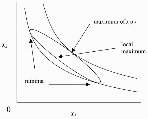
2.3 Product of two state variables

This covers, for instance, derivation of bounds on the vertical velocity component of a target from bounds on its velocity and the cosine of the angle of the velocity to the local vertical, convenient state variables in ballistic flight. To find the extremes of x ₁ x ₂ over

, an analysis along similar lines to that in Section 2.2 gives

where now

The small increase in complexity of d leads to a quartic for d in terms of the first two elements of

and the top left 2 × 2 partition of P:

where

An exact solution of equation (13) is available by several classical methods [9]. The extremes of x ₁ x ₂ follow by solving the linear equation (11) for x ₁ and x ₂ in terms of d, then forming x ₁ x ₂ directly or, to get a slightly simpler expression, using equation (12) again to give

The nature of the stationary points of x ₁ x ₂ on the boundary of

is seen by examining the values of the Lagrange multiplier λ = – d/2 at the roots of equation (13). They comprise either (i) a complex conjugate pair, a negative, real value yielding the minimum and a positive, real value giving the maximum, or (ii) four real values: a positive value at the global maximum, a negative value at the global minimum, another negative value at a local minimum, and a negative value at a point which is a local maximum with repect to x ₁ and x ₂ but a minimum with respect to the other state variables. The global maximum is at the unique point of external tangency of the strictly convex

and a convex set of the form x ₁ x ₂ ⩾ c. Any minimum is at a point where

is a tangent from the interior to a set of the form x ₁ x ₂ ⩾ c, so in (ii), the pair of minima may be distinct yet coincide in value, as in figure 2 and the example below.

Figure 2. Points corresponding to roots of equation (13).

Example. The extreme points of x ₁ x ₂ on the boundary of

are required, where

has centre

and describing matrix

In equation (13) α = 18.0655, β = 6.2955, γ = – 15.0545 yielding roots d′= 2.509091, 2.509091, – 4.244288 and – 0.773894. The corresponding points x ^T  = [5 0.2 …], [0.5 2 …], [3.723 1.489 …], [2.277 1.971 …] are respectively two global minima, the global maximum and a local maximum between the minima. Δ

2.4 Positive-semidefinite quadratic form

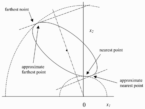
The extremes of x ^T Qx on the boundary of the ellipsoid

, for Q symmetric and positive-semidefinite or definite, are useful in a number of situations. They include as a special case bounds on the range of a target with Cartesian position components and their derivatives as state variables. More generally, tests for the intersection and inclusion of ellipsoids can be based on these extremes. With Q positive definite, if

, one can check whether the ellipsoids

and

intersect by examining the minimum of x ^T Qx subject to

. If

, the minimum shows whether

. Such tests appear in Section 3.

The case where

contains a point in the null space of Q (such as the position origin in the range-bounding case) is uninteresting, as the minimum of

subject to

is then zero. Excluding this case, the extreme points of x ^T Qx can be found by setting the derivative ∂L/∂x of the augmented cost function

to zero, yielding

The inverse in equation (17) exists unless λ is an eigenvalue of PQ. In that case, the origin, the centre

of

and the point where

and

touch are collinear on the eigenvector associated with λ. Such cases are detectable by noticing that

is an eigenvector of PQ, and the location and value of the extreme of x ^T Qx are found from the corresponding eigenvalue.

In the generic case, premultiplying ∂L/∂x = 0 by

and setting

gives

From equation (17),

so

becomes

This polynomial in scalar λ is solved; then, x follows from equation (17), yielding a bound

on

. In general, equation (19) is of degree 2n in λ and requires a root-finder if n > 2.

Computational cost may inhibit the use of equations (19) and (20) in conjunction with recursive state estimators at high update rates, so economical approximations may be useful. A very cheaply computed one is found by noticing that the terms of degree 2n and 2n – 1 in λ in the polynomial equation obtained by rationalizing equation (19) are those of |PQ – λI|², namely λ ²ⁿ ,− 2tr(PQ)λ^{2 n  – 1}. Hence, for a dominant root | λ| >> 1 an approximate solution is

.

The points of

closest to and farthest from a given point x* not in it are found by putting I for Q and

for

. They may be approximated by the extreme points

in direction

, using equation (3). This approximation is clearly good when the distance from x* to

is much longer than the longest half-axis

of

.

Example. The points of

farthest from and nearest to the origin are required, where

has centre

and describing matrix

Straightforward calculation gives:

Substituted into equation (19) with Q = I, this gives, after tidying up,

The only real roots are λ = 11.9031, – 2.1247. The positive value indicates that x ^T x increases if the bound on

is increased from 1, so it applies at the farthest point of

from the origin, and the negative root gives the nearest. Through the second part of equation (22), the extremes are, respectively, x ^T  = [ – 2.6731 4.6114], [0.0679 1.2703].

The simplest approximation

is fairly close to the larger root and gives as the farthest point x ^T  = [ – 2.2453 4.2264]. The other approximation

gives

 = [− 2.5250 4.6775], quite good given that the distance from the origin to

is only 3.162, comparable with the length 2.358 of the longer half-axis of

. The approximation

 = [0.5250 1.3225] to the nearest point is less good absolutely as well as relatively. Figure 3 sketches the situation, showing the extreme points and second approximation.

Figure 3. Points of nearest to and farthest from origin, and approximations.

3. Operations on state-bounding ellipsoids

3.1 Test for intersection and inclusion of ellipsoids

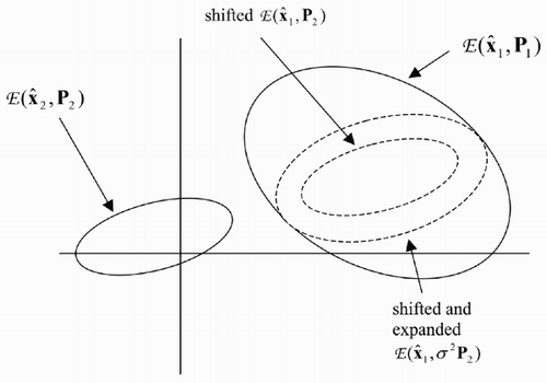
Results (17), (19) and (20) provide tests for inclusion and intersection of general ellipsoids

and

. They can be used directly, putting P ₁,

for P, Q and

. Alternatively, they can be simplified by an affine transformation

where

, which transforms

to the unit ball

centred at the origin, so Q = I, and transforms

to

where

replace P and

. This option is adopted here to minimize algebra. The following tests are then obtained.

Test 3.1.1

Does

contain

? If

, then

. This is so if and only if (i) the origin is in

and (ii) the point of the boundary of

nearest the origin is at least distance 1 from it. Hence

contains

iff

and (putting Q = I,

in equations (17) and (19))

Moreover, if tests (25) and (26) are passed, the largest factor by which

can be expanded and stay contained in

is

. As ratios of distances in the same direction are unchanged by affine transformation, this is the largest ratio by which

can be expanded and still be contained in

.

The following complementary test to Test 3.1.1 reuses the affine transformation.

Test 3.1.2

Does

contain

? If

then

. This is so if and only if the distance of the farthest point of the boundary of

from the origin is no greater than 1. From equations (17) and (20), this is so iff

If Test 3.1.2 is passed, the largest ratio by which

can be expanded and still be contained in

is

, which is the largest ratio by which

can be expanded and remain in

.

Test 3.1.3

Does

intersect

? If

, then

. This is so if either (i) the distance of the nearest point of the boundary of

from the origin is no greater than 1 or (ii)

. The test is thus whether

or

Test 3.1.4

Are

and

disjoint? If

then

. This is so if Test 3.1.3 is failed, but an equivalent test is whether

does not contain the origin (or any other test point of

; the origin is the simplest to test), and the distance of the nearest point of the boundary of

to the origin is greater than 1, i.e.

The smallest factor by which

must be expanded to intersect

, and hence the smallest ratio by which

must be expanded to intersect

(but not vice versa) is

.

3.2 Largest expanded ellipsoid of given shape in a given ellipsoid

The problem is to find

and the greatest scalar σ such that

, given

. That is, find the largest scaled and shifted version of an ellipsoid with describing matrix P ₂ which will fit into

.

By symmetry,

, and the ellipsoids

and

touch when the ratio

of the distances in direction ϕ from their joint centre

to their boundaries is unity. Now

so

Figure 4 illustrates a two-dimensional case.

Figure 4. Largest shifted and expanded version of ellipsoid inside .

Example. Given

the largest scaled version of

fitting into

is required.

The eigenvalues of

are 12.8146, 0.3814 and 0.1790, so

0.4231, and

has to be shrunk in this proportion to fit into

.

3.3 Worst-case-reachable set

The worst-case-reachable set comprises all future state values reachable, by the exercise of bounded forcing, from every point in the current feasible set. If the effect of forcing is additive (as in any system which is linear in additive forcing), the set is

That is, every point in

is reachable from any starting point in

by adding an increment (due to forcing) from

. It is convenient to approximate

and the bounded forcing by ellipsoids, but the forcing may be of lower dimension than the state. If so,

with F positive-semidefinite. Whether or not F has full rank,

is generally not an ellipsoid but must be approximated by the largest (maximum-hypervolume) ellipsoid

Denoting the vector sum of sets

by

, (34) implies and is implied by

The largest ellipsoid

in the ‘vector difference’ of

can be found as follows, by a derivation much like that for the smallest ellipsoid containing the vector sum of two ellipsoids ([5], appendix A). If

were zero, the centre of

would be the origin, by symmetry. Non-zero

simply add

to every vector in

and subtract

from every vector in

, adding

to every point of

, so for the centre of

choose

To permit an analytical solution for

, we require R to be linear in S and F:

The width

of

in any direction φ must not be less than the sum of the widths g_s, g_r of

and

in that direction, so using equation (37),

so

or, defining ρ ≡ g_f /g_s  ⩾ 0 (permissible as S > 0),

With g_s  > 0 and g_f  ⩾ 0,equation (39) requires at least one of α/β and 1/β to be greater than unity. It is easy to confirm that equation (40) is satisfied by

closely analogous to the choice in the standard vector-sum algorithm [1, 5]. Hence,

The final step is to find the value of p maximizing the hypervolume of

, proportional to |R|. Its maximum is where

As |R| is not zero, the trace in equation (43) must be zero, giving

so, after some manipulation,

Noting that tr(A + B) = tr(A) + tr(B), this yields

where n is dim(x). As

, (46) gives

A root-finder solves this polynomial equation for p; then, equation (42) gives R for each positive root, and the one giving the largest |R| is selected. Δ

4. Illustrative use of results

4.1 Interception subject to uncertainty in threat trajectory

Terminal-phase guidance laws for ballistic-missile interceptors do not take account of longer-range factors such as target selection or economical use of fuel for manoeuvring. Control schemes with the potential to include these factors in mid-course navigation of the interceptor, through periodically updated constrained optimization of the interceptor's planned trajectory, are approaching computational practicability. In such schemes, the performance of the interceptor may be made less sensitive to uncertainty in the predicted target trajectory by two strategies. One is to rely on the feedback provided by periodic correction, reoptimizing the interceptor trajectory in the light of up-to-date observation of the target and applying each successive optimized control sequence only up to the next observation. The second strategy is to account explicitly for the uncertainty during the optimization. This is desirable if a number of candidate targets must still be considered, weighted by their perceived threat and the uncertainty in their trajectories, or if the uncertainty is large enough to pose a large risk, if ignored, that the control action is inappropriate even in the short term.

When uncertainty is included in the optimization, a worst-case optimality criterion suits interception. The predicted situation closer to interception is to be optimized in the most difficult case over the bounded uncertain future state of the threat. This has some similarity to employing a game-theory formulation of the problem [10], but the connection will not be pursued here. The uncertain threat state prediction may be updated relatively easily, as new sensor measurements arrive, if it is in the form of an ellipsoidal feasible set

[5, 7]. If uncertainty in predicting the interceptor state can be neglected, the guidance optimization needs to evaluate some measure of the discrepancy between the future controlled interceptor state and the most unfavourable future threat state, e.g. the largest possible range of the threat from the interceptor. The results of Section 2.4 give this discrepancy so long as it is expressed as the maximum of a weighted quadratic norm of the threat state with respect to interceptor state. The second approximation suggested in Section 2.4 can be employed while

covers a small proportional range of the weighted quadratic norm, which will normally be so until late in the engagement, by which time a simple terminal guidance law will have been initiated.

4.2 Interception with uncertainty in trajectories of both threat and interceptor

If the interceptor state is also significantly uncertain, worst-case-optimal guidance requires the maximum difference between the two states over both feasible sets. Generalizing Section 2.4 to find the maximum, over two ellipsoids, of a non-negative-definite quadratic form in the state difference is algebraically and computationally complex. Instead, the simpler strategy of making the predicted interceptor feasible set (usually much the smaller) first intersect that of the threat then be contained in it, positioned by some subsidiary criterion, is attractive. This requires the tests in Section 3.1.

4.3 Gauging of requirements to meet the control objective

The results of Section 3.2 indicate what nominal final state maximizes the permissible uncertainty about this value while still meeting a terminal control condition, expressed as an ellipsoidal set of acceptable final state values. It also gives the size of that uncertainty. It could, for instance, be used to indicate the change in nominal future interceptor state and the reduction in its uncertainty required to ensure that the interceptor comes close enough to the threat to guarantee successful interception.

4.4 Interception employing worst-case-reachable set

Computation of the worst-case-reachable set of the interceptor at each update allows the control sequence and choice of target to be optimized in full knowledge of the range of outcomes achievable. In the early stages of an engagement, the control can aim to keep as many objects as possible within reach of the interceptor or to keep specific objects reachable for as long as possible. Once the target is selected, a simple worst-case-optimal strategy is to make the reachable set at the predicted interception time cover, in the subspace of the state variables appearing in the control objective (including position components), as large an expanded version of the threat's feasible set as possible. That is, the range of future threat behaviour (about its predicted, perhaps optimistic, feasible set) over which interception is guaranteed is maximized.

Section 3.3 gives the largest ellipsoidal internal approximation to the set reachable in the worst case from an ellipsoidal feasible set by additive, ellipsoidally bounded forcing.

5. Conclusions

A number of results, with some approximations to reduce computational load, have been presented for deriving bounds on scalar state-dependent quantities from the ellipsoidal bounds produced by standard state-bounding algorithms. Tests of intersection and inclusion of ellipsoids have been based on them. An algorithm for computing an ellipsoidal worst-case-reachable set has also been obtained, and some ways in which these results might be employed in interception problems have been discussed to illustrate their potential.

Acknowledgements

This material results in part from work supported by the UK Ministry of Defence. The advice and encouragement provided by Martyn Bennett of dstl, Farnborough, are gratefully acknowledged.

References

- Chernous'ko , F . 1981 . Optimal guaranteed estimates of indeterminacies with the aid of ellipsoids. I, II . Engineering Cybernetics , 18 : 1 – 9 .
- Chernousko FL 1994 State Estimation for Dynamic Systems Boca Raton FL CRC Press
- Durieu C Polyak BT Walter E 1996 Paper presented at Proceedings of the 13th Triennial IFAC World Congress San Francisco CA
- Kurzhanski AB Valyi I 1997 Elliposidal Calculus for Estimation and Control Boston MA Birkhäuser
- Maksarov , DG and Norton , JP . 1996 . State bounding with ellipsoidal set description of the uncertainty . International Journal of Control , 65 : 847 – 866 .
- Maksarov , DG and Norton , JP . 2002 . Computationally efficient algorithms for state estimation with ellipsoidal approximations . International Journal of Adaptive Control & Signal Processing , 16 : 411 – 434 .
- Pronzato , L and Walter , E . 1994 . Minimum-volume ellipsoids containing compact sets: application to parameter bounding . Automatica , 30 : 1731 – 1739 .
- Schweppe , FC . 1968 . Recursive state estimation: unknown but bounded errors and system inputs . IEEE Transactions on Automatic Control , AC-13 : 22 – 28 .
- O'Connor JJ Robertson EF 1996 Quadratic, cubic and quartic equations Available online at: http://www-history.mcs.st-andrews.ac.uk/history/HistTopics/Quadratic_etc_equations.html (accessed 16 December 2003)
- Anonymous news release: New research analyzes the game of missile interception 10 July 2000 Available online at: American Technion Soc, http://www.ats.org/news.php?id = 13 (accessed 10 March 2004)