Modelling and hierarchical diagnosis of timed discrete-event systems

Abstract

A new diagnostic method for hierarchically structured discrete-event systems is presented. The efficiency of this method results from the fact that the complexity of the diagnostic task is reduced by first detecting a faulty component using a coarse process model on a high level of abstraction, and subsequently refining the result by investigating the faulty component with the help of a detailed component model in order to identify the fault with sufficient precision. On both abstraction levels, the method uses a timed discrete-event model of the appropriate part of the system. On the higher abstraction level a timed event graph is used that describes how the temporal distance of the events is changed by component faults. On the lower level of abstraction, timed automata are used to cope with the non-determinism of the event sequence generated by the faulty and faultless components. The approach is illustrated by the diagnosis of a batch process.

Keywords:

• Time discrete-event modelling
• Hierarchical diagnosis
• Timed automata
• Timed event graphs

1. Introduction

Process diagnosis is the task of detecting and isolating faults in technical processes from measured input and output data. A model-based diagnostic algorithm uses an explicit model of the dynamical system under investigation ( figure 1). This model incorporates the knowledge about the faultless and the faulty system behaviour.

Figure 1 The principal structure of model-based diagnosis.

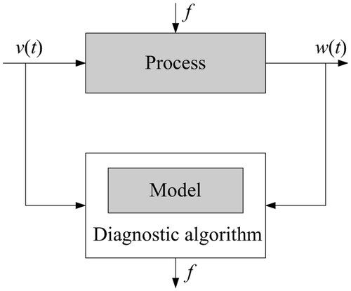
This paper is concerned with discrete-event systems whose inputs v, states z and outputs w have discrete value spaces. Likewise, the faults f are considered to be discrete phenomena. Such systems are commonly found in manufacturing or chemical engineering, where actuators influence the process by initiating discrete command signals and sensors provide discrete measurement values of, for example, position, level or temperature to the controllers and the process supervision systems. The dynamical behaviour of such systems is characterized by sequences of discrete events that represent changes of the discrete-variable inputs, states or outputs at certain time instants. Therefore, the models used in diagnosis have to describe the evolution of the given system in terms of untimed or timed event sequences.

In recent literature, various diagnostic approaches to the solution of the diagnostic problem for discrete-event systems have been developed. These methods differ with respect to the modelling paradigm, the use of timed or untimed models, the interpretation of the fault in the model and the complexity. An overview of the diagnosis of discrete-event systems is given in 1. In 2 and 3, the fault is explicitly modelled as a fault event in an untimed or timed automaton, respectively, and the diagnosis consists of detecting the occurrence of a particular fault event. In contrast, faults are detected from the deviation of the measured timed event sequence from given template languages in 4 or the firing sequence of a timed Petri net in 5. The principle of consistency-based diagnosis has been applied in 6 to timed discrete-event systems described by semi-Markov processes. The fault is modelled implicitly in terms of its effects on the system behaviour.

The issue of complexity reduction in model-based diagnosis is addressed in 7 by representing a model in the form of logic programs at several levels of detail which leads to the formulation of a hierarchical diagnostic algorithm. An alternative approach for discrete-event models has been presented in 8 and in more details in 9 for untimed discrete-event systems and explicitly modelled fault states. The diagnosis does not require a model of the overall process or a global diagnoser as in 2 but decomposes the problem into less complex subproblems by treating systems as assemblies of components. A decentralized diagnostic architecture is presented in 10.

The method presented in this paper uses a hierarchical model and the diagnostic methods that are appropriate for the models at the different hierarchical levels. As large-scale systems as well as their control equipment typically possess a hierarchical structure, the behaviour of the modules on different hierarchical levels is represented by different discrete-event models that are appropriate to the different abstraction levels along the system hierarchy. While on the lower level of the process, component models should describe physical quantities, on the higher level only sequences of global processing steps executed by these components are of interest for the diagnoser. For the representation of the timed discrete-event behaviour of the components, timed automata are used whereas the global system behaviour is modelled by a timed Petri net. The latter describes the process as a whole and does not contain the detailed behaviour of each process component. This hierarchy with a rough model of the overall system and detailed models of the components reduces the information to the amount necessary for diagnosis on these abstraction levels. On the upper level the existence of a fault is detected and the set of possibly faulty components is isolated based on the coarse model. The detailed component model at the lower level is subsequently used to identify the fault, thus refining the diagnostic result.

This paper is organized as follows: Section 2 states the diagnostic problem for timed discrete-event systems. After the main ideas of the solution to the diagnostic problems at both hierarchical levels have been presented in Section 3, Section 4 introduces the two modelling paradigms followed by a presentation of their integration to form a hierarchical model for the diagnostic purpose. According to the modelling hierarchy, the diagnostic task is solved in two steps as described in Section 5. Finally, the effectiveness of the hierarchical diagnosis is illustrated in Section 6 by applying the method to a batch process.

2 Diagnostic problem

Discrete-event systems are dynamical systems with a discrete state space where the state evolution depends on the occurrence of events 11. Similar to the states z, the input values v and output values w of the discrete-event system are considered as discrete quantities. Thus, v, z and w can be enumerated as follows:

where , and represent the sets of inputs, states, and outputs, respectively. The changes of states will be considered as events. represents the finite set of events which can occur. Figure 2 illustrates a possible sequence of events generated by a system with . The dash at the lower part of the figure shows the events e(0), e(1),…, e(4) and the time instants T(0),T(1),…,T(4) at which these events occur.

Figure 2 Event generation in discrete-event systems.

This paper concerns timed discrete-event models, in which not only the order of discrete events but also the sojourn time between the events is important. The timed event sequence

marks the transitions from one discrete state to another within the time interval [0, t_h ]. The system evolution is influenced by a discrete-valued input sequence

and its behaviour is observed as a discrete-valued output sequence

where T(k) denotes the time instant at which the k-th change of a signal occurs. Obviously, one can obtain untimed sequences from the timed descriptions by neglecting the temporal information. Note that synchronous discrete-event systems are considered, where any change in the input or output sequence can occur only at the same time with some event e. This means that the time points T(k) are the same in the event, input and output sequences (2) –  (4).

In order to describe the faulty discrete-event system, the set of discrete faults

is introduced. Unlike the sets defined in (1), includes 0 to denote the case where no fault is present in the system. Faults occurring in a discrete-event system may affect the event sequence in two respects:

	A fault changes the temporal distance between the events. This change is typical for small fault magnitudes where the system remains in operation and follows the same event sequence as in the faultless case but changes the temporal distance between events.
	A fault changes the causal order of the events. Such fault effects are typical for large faults which change the event order or enable some unexpected events.

Both fault effects can be represented by the timed automaton used as component model later on, whereas only the first effect can be described by the timed event graph used to represent the overall system behaviour.

With the notations given above, the diagnostic problem can be formulated as follows:

Table

	Diagnostic Problem
Given:	Timed discrete-event model
	Timed input sequence V(0…th )
	Timed output sequence W(0…th )
Find:	Fault f

This problem will be solved for hierarchical systems, where at each hierarchical level the relevant model and the relevant timed input and output sequences will be used.

3 Hierarchical diagnosis

3.1 Main idea

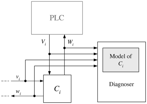
This paper considers dynamical systems, which are controlled by programmable logic controllers (PLC) as illustrated in figure 3. The system consists of a set of interconnected components C_i . These components interact with each other, interchanging material, energy or information. This interaction at the component level for a component C_i is represented by the signals v_i and w_i where v_i describes the influences of the components C_j (j ≠ i) on the component C_i and w_i represents the output of C_i which may affect other components.

Figure 3 System to be diagnosed.

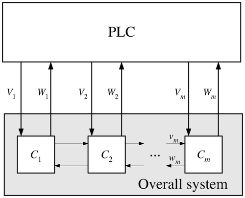
At the overall system level, the PLC controls the system by discrete-valued inputs V_i acting on the component C_i . All component inputs together form the input

to the overall system. Likewise, the outputs W_i of the components C_i are collected in the overall system output

In figure 3, the input V and output W include only the information required by the PLC in order to control the system behaviour in a predefined way. V and W are subsets of the set of signals received and generated by the components . The input signal received by the component C_i consists of the input signal V_i from the PLC and the coupling signals v_i that describe the influence of all other components C_j (j ≠ i) on the component C_i . Similarly the output signal from the component C_i contains both W_i and w_i . Therefore, it is obvious that the amount of information available on the component level is more detailed than that required by the supervision system.

The diagnostic method introduced in this paper uses this hierarchical structure to decompose the diagnostic problem into two steps:

1. The occurrence of a fault is detected by considering only the overall system behaviour given by V and W and a set of candidate components for a detailed diagnosis is determined.

2. This step refines the diagnostic results by performing a detailed diagnosis for the components by means of the input V_i and output W_i relevant to C_i and the additional signals v_i and w_i describing the interconnection with other components. The aim of this step is to determine the exact location of the fault.

Accordingly, in the diagnostic problems to be solved at the overall system level or at the component level, the sequences

or

respectively, are available.

3.2 Diagnostic problem for the overall system

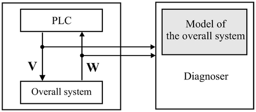
The overall system is considered from a process-oriented viewpoint. At this level of abstraction, the system behaviour is described by sequences of processes each of which is executed by one component or by several components together. In order to satisfy the technological goals, the PLC enforces a specified sequence of processes by issuing commands V while receiving information about the status of the running processes via the signals W as shown in figure 4.

Figure 4 Overall system diagnosis.

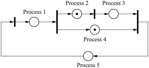
In practical applications, especially in manufacturing and process industries, several processes are executed synchronously, while concurrency is eliminated by the PLC. This means that the sequence of events which occur at the level of overall system is predefined and the behaviour of the overall system can be determined by the time at which each event has to occur. Therefore, the overall system can be appropriately described by a timed event graph 12, whose places represent the processes and their duration and whose transitions describe the beginning or termination of these processes as shown in figure 5. Details will be explained in Section 4.1.

Figure 5 Representation of the sequence of processes by a timed event graph.

A fault in one component C_i typically changes the duration of a process and hence the temporal distance of events. In the worst case the component cannot carry out its job at all and hence has an infinite processing time. By monitoring the process durations, the diagnoser detects the presence of a fault in the overall system. To do so, the diagnoser evaluates the timed sequences of inputs V and outputs W of the overall system by means of an overall system model.

3.3 Diagnostic problem for components

Once the diagnosis of the overall system has determined the candidate set of faulty components , a more detailed diagnosis of these components will be triggered. The principle of the diagnosis at the component level is illustrated in figure 6 where the component is under consideration. C_i receives the control signal V_i  ∊ V from the PLC and contributes the output W_i  ∊ W to the overall system level. In addition, the component C_i also generates the output w_i to other components j (j ≠ i) and receives the coupling signal v_i from other components j (j ≠ i). The diagnoser of the component C_i uses the signals V_i , W_i , v_i and w_i to identify the fault. Hence, only the signals which are relevant for the component C_i are used. Other signals from V and W at the overall system level not crucial for the component C_i are void.

Figure 6 Diagnosis at the component level.

The discrete-event behaviour at the component level is, in general, non-deterministic. Therefore, timed automata are used to describe the individual components. In addition, multiple transitions of a timed automaton from one initial state to all potential successor states can be interpreted as several operating modes of a process component.

4 Timed discrete-event models for diagnosis

4.1 Timed event graphs as models on the higher hierarchical level

The model considered for the description of the overall system behaviour is a timed event graph. Timed event graphs are Petri nets where each place has precisely one upstream transition and one downstream transition (for details see 12). Each place represents a process that occurs in the technical system under consideration. The marking of the places by tokens indicates which processes are active whereas the firing of a transition indicates the activation of the processes represented by the places downstream of the transition. A holding time associated with each place describes the duration of the corresponding process and thus the minimum time a token must spend in a place before contributing to enable the transition downstream to this place.

The timed-event behaviour is described by the daters x_i (k) and u_j (k), where x_i (k) denotes the time of the k-th firing of the transition q_i and u_j (k) the firing time of the input transition . An input transition is a transition with no predecessor places. Its firing time does not depend on the system state. We will assume in the sequel that the signals u_j (k) are determined by the PLC.

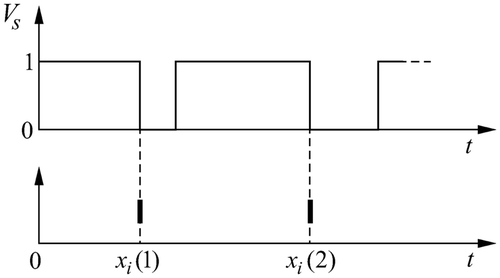
As the daters x(k) and u(k) mark the activation of the processes, they correspond to particular changes in the signals V and W as illustrated by an example in figure 7. It shows that the dater x_i (k) denotes the k-th time instant at which the signal V_s changes from 1 to 0. Therefore, for a given system and a given sequence of processes there exist transformations and that transform the discrete valued sequences V and W into the daters x(k) and u(k).

Figure 7 Changes in signal V_s and corresponding dater x_i (k).

The evolution of the daters x_i (k) in timed event graphs can be described algebraically as follows (for details see 12). Consider the initial marking of the timed event graph on the left-hand side and the event sequence given on the right-hand side of figure 8. The token in the place p_ir has been produced by a firing of the transition q_r prior to the beginning of the system observation. By convention, this event is identified by the event counter k = 0 such that this particular event time is x_r (0). The first firing of transition q_i occurs at time x_i (1) only if transition q_j and input transition have fired for the first time (x_j (1) and u_j (1)) and the holding times τ _ij , and τ _ir in the downstream places p_ij , and p_ir have elapsed. The same reasoning holds for the relation between x_i (k + 1), x_j (k + 1), u_j (k + 1) and x_r (k):

This equation is linear in the max-plus algebra 12, 13. The operators of the max-plus algebra ⊕ and ⊗ are defined by

The identity elements of max-plus addition ⊕ and max-plus multiplication ⊗ are −∞ = ε and 0, respectively. Note that ε is absorbing with respect to ⊗. The matrix addition and multiplication are defined similarly to the conventional algebra.

Figure 8 Part of a timed event graph and potential event sequence.

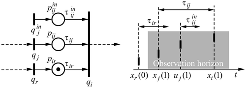
As described above, the marking of a place indicates whether or not a process is active. Thus, each place contains at most one token in the initial marking. In addition, we assume that each downstream place of each input transition is initially unmarked. 1 Then the daters x_i (k) (i = 1,…, n) representing the internal events of the system and the daters u_j (k) (j = 1,…, p) modelling the input events satisfy the implicit equation

The entry (A ₀) _ij and (A ₁) _ij of the matrices A ₀ and A ₁ is equal to the holding time τ _ij of the place p_ij which is downstream to q_j and upstream to q_i if the place is initially unmarked or initially marked, respectively. Similarly, the entry (B ₀) _ij is equal to the holding time of the place downstream to the input transition . If no place connects transition q_j or to q_i then the corresponding matrix entry is equal to ε.

Equation (6) relates the holding times corresponding to process durations collected in the matrices A ₀, A ₁ and B ₀ to the measured event times x(k + 1) and x(k) and the given input event times u(k + 1). A difference between the observed event time sequence and the event time sequence generated by the model indicates a change of holding times. Thus, the occurrence of a fault is modelled as a deviation of the holding time corresponding to a particular process from a given reference value. This interpretation will be used in Section 5.1 to detect a fault by comparing estimated holding times with given reference values.

4.2 Timed automata as models on the lower hierarchical level

To identify the fault in a system component, a more elaborated model of the component is necessary. Timed automata, which are finite state machines with timed transition behaviour, will be used 14. To model the system component for diagnosis, a timed automaton is extended to describe the relation between inputs, coupling signals and outputs under the effects of different faults.

A timed automaton is denoted by the 7-tuple

with the finite sets , , and as described in Section 2. T _h is the time interval for which the automaton is defined and R is the transition relation of the automaton. is the initial state.

If the automaton describes the component C_i , the states of the automaton represent the internal states of the component. The input v to the automaton includes both the control input V_i from the PLC and the coupling signal v_i (see figure 6). Similarly, the output w of the automaton consists of the outputs W_i and w_i . These facts can be represented by two mappings M_v and M_w :

The transition relation R which describes the dynamical behaviour of the automaton subject to a fault f is given by

The variable τ ∊  T _h describes the sojourn time in the state z of the timed automaton with the fault f while receiving the input v before the automaton makes an instantaneous transition to state z′ and generates the output w.

In general, the sojourn time τ(z′, w, z, v, f) is uncertain and expressed as the time interval that the automaton has spent in z before the transition to z′ takes place

where τ_min(z′, w, z, v, f) and τ_max(z′, w, z, v, f) are the lower and upper bounds for a possible occurrence time of a state transition. The interval [τ_min(z′, w, z, v, f), τ_max(z′, w, z, v, f)] is defined for any pair of states and inputs (z, v) for which there exists a successor state z′ and an output w such that R(z′, w, τ, z, v, f) = 1 holds. For R(z′, w, τ, z, v, f) = 0, τ(z′, w, z, v, f) is not defined.

For a given component, the timed automaton can be obtained, for example, by abstraction from a given quantitative model that describes the behaviour of the physical system quantities or by identification if experimental data are available 15.

The graphical representation of an automaton is the automaton graph, where each state is represented by a node. The edges connecting the nodes describe the state transitions corresponding to z′, w, τ, z, v, and f for which R(z′, w, τ, z, v, f) = 1 holds. The left part of figure 9 illustrates an automaton graph for a faultless system (f = 0) with four states, two possible values for v and three possible values for w. The solid and dashed edges in the automaton graph represent the possible transitions for v = 1 and v = 2, respectively. The ticks in the right part of the figure represent the time instants when the automaton makes a transition from one state to another.

Figure 9 A timed automaton and one of its possible state sequences.

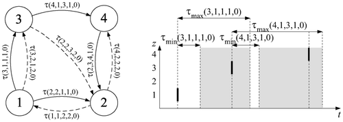
The state evolution of this timed automaton for f = 0 can be described as follows: Let z ₀ = 1 be the initial state. For v = 1, a transition to state z = 2 or z = 3 is possible. The transition to z = 3 must occur within the time interval τ(3, 1, 1, 1, 0), which means the earliest at τ_min(3, 1, 1, 1, 0) and the latest at τ_max(3, 1, 1, 1, 0) as shown in the right of figure 9. If this state transition occurs, the output value w = 1 is generated.

To this end it is assumed that both models of the overall system described by the timed event graph and the component model described by the timed automaton are complete in the sense defined in 6. This means that the model generates all the event and output sequences that the system may generate over the same timed horizon for the same initial event, input sequence, and fault.

5 Integration of two diagnostic methods for hierarchical diagnosis

This section elaborates the main idea described in Section 3 in detail. First, the two diagnostic methods based on the models described in Sections 4.1 and 4.2 are presented. Then, Section 5.3 describes the integration of these two approaches to a hierarchical diagnostic algorithm.

5.1 Parameter estimation for overall process monitoring

In this section, a method is developed for solving the diagnostic problem for the overall process modelled by a timed event graph. This method uses the N + 1 last state event times and N last input event times which form the sequences

Table

	Fault detection problem for the overall system
Given:	Model of the overall system (6)
	Sequences of event times X(k − N…k) and U(k − N + 1…k)
Find:	Set of possibly faulty components

As discussed in Section 4.1, the effect of a fault is interpreted as a change of a parameter in (6). Therefore, residuals defined as the deviations of estimated values for the entries in the matrices of (6) from given reference values provide the information about the set of possibly faulty components.

A first solution to this problem was introduced in 16 using a particular equation error for parameter estimation (for earlier parameter estimation approaches see 17 and the references cited therein). However, the proposed method provided only heuristic solutions to the following problems:

1. To obtain reliable residuals, all estimated parameters should be equal to their corresponding true values. However, in general the parameter estimation algorithms for the considered system class give only an upper bound. This problem can be overcome by applying one of the methods given in 18 to determine particular input signals, similar to the concept of persistent excitation known from conventional system identification.

2. The parameter estimation requires measured event times. However, for particular fault types or fault magnitudes the system may stop generating additional events.

To overcome this problem, a residual generation method that enables a residual determination even in the case that the process ceases to generate events is presented here 18. Before this extension is described, the parameter estimation method given in 16 is reviewed. Let

be the estimates of the system matrices occurring in (6) and the measured event times and given input event times, respectively. Then the following equation error ξ(k + 1) is determined after the observation of the (k + 1)-st firing of each of the transitions:

As the vector m(k + 1) contains the firing times x(k + 1), x(k) and u(k + 1), it can be determined similarly to x(k) and u(k) using the transformation .

The following considerations illustrate how the estimates for the system parameters can be determined.

Consider the i-th line of Equation (6). By recalling that ⊕ and ⊗ represent conventional maximization and addition, respectively, it can be seen that

holds for all i, j, k. Thus, an upper bound for the parameter Θ _ij is obtained from

The least upper bound that results from the most recent N measurements of x(k) and m(k), collected in the matrices

is now defined as the estimate:

Note that this corresponds to the greatest solution of the inequality

12, 13. Due to (15) the solution determined by (16) satisfies the relation

Since the operation ‘⊗’ is isotone, one obtains for a constant matrix Θ

by using (17) 13,17. Thus,

holds. From (19) it follows immediately that the equation error vanishes ξ(ν) = 0, for all ν = k − N + 1,…, k. Thus the solution given by (16) minimizes the equation error if the matrix Θ is constant. With the occurrence of a fault Θ changes. Then the equation error is no longer zero. However, Equation (16) still provides the true system parameter values, meaning that (18) holds with equality, if the system is subject to an adequate persistent excitation. Three methods to compute a persistent excitation have been introduced in 18. In addition, the choice of an appropriate value for N, the number of measurements considered for parameter estimation, has been discussed.

Denote by

the dater [xcirc]_i (k) predicted by the model estimated at the end of the (k − 1)-st cycle. The residual for Θ _ij obtained in the k-th cycle is now defined as:

If x_i (k) ≤ [xcirc]_i (k) + Δ _ij holds, which means that the k-th firing of transition q_i occurs earlier than predicted by the model estimated in the previous cycle or is delayed less than Δ _ij , this residual is equivalent to the residual already defined in 16. Otherwise, the k-th firing of q_i is delayed by more than Δ _ij with respect to the time [xcirc]_i (k) predicted by (20). This includes the case of an infinite delay meaning that the k-th firing of q_i never occurs. Then

holds and the resulting residual deviation indicates the occurrence of a fault even in this case. Note that if the reference values Θ _{ij, Ref} are not known a priori, they can be determined using (16) from measurements x(k) and m(k) of the faultless process.

The algorithm presented subsequently describes how the residual r_ij is determined. We will assume that the persistent excitation of the process is such that the true value of each parameter can be determined within N process cycles. During the first N − 1 measurements of x(k) and m(k) no parameter estimation is performed as we cannot be sure that the estimated values are equal to the true parameters. Therefore, the residuals in the first N process cycles are set to zero. After the measurement of x(N) and m(N) we always can determine estimates based on N measurements and therefore obtain reliable residuals.

Algorithm 1. Monitoring of the overall system using parameter estimation

• Given:  –  Timed event graph that describes the overall system behaviour

•  – Nominal parameters Θ _{ij, Ref}

•  – Transformations ,

•   – Threshold δ _ij  > 0 for residual evaluation

• Initialize:Set X, M as empty matrices

• While  k < N:

  1. measure next event time

  2. if is measured, append M by m_r (k) determine [xcirc]_i (k) using (20)

  3. If t ≤ [xcirc]_i (k) + Δ _ij then

     • if is measured, append X by x_i (k)

     else r_ij (k) = Θ _ij,Ref − [xcirc]_i (k) + m_j (k) − Δ _ij

• While  k ≥ N:

  1. measure next event time

  2. if is measured, append M by m_r (k) determine [xcirc]_i (k) using (20)

  3. If t ≤ [xcirc]_i (k) + Δ _ij then

     • if is measured, append X by x_i (k) determine from (16)

     else r_ij (k) = Θ _ij , Ref − [xcirc]_i (k) + m_j (k) − Δ _ij

  4. Remove old entries from X and M

• Result: Set of possibly faulty components corresponding to the residual |r_ij | ≥ δ _ij .

The threshold δ _ij is introduced to cope with uncertainties in the system parameters for the faultless case. The residual r_ij which is greater than δ _ij indicates that a fault must have occurred in one or more components involved in the execution of the process represented by the parameter Θ _ij . Thus, this algorithm detects a fault in the system and determines the set of components that are candidates for a detailed component diagnosis. As the cardinality of typically is much lower than the cardinality of , this step also yields a rough fault isolation.

5.2 Fault isolation and identification of process components by consistency-based diagnosis

To isolate and identify the fault at the component level, the model in the form of timed automata introduced in Section 4.2 is used. The paper applies the idea of consistency-based diagnosis for timed automata elaborated in 19 for fault isolation and identification.

Until the diagnostic algorithm for overall process has not detected any faults, the diagnosis at the component level is idle. It is triggered after the diagnoser on the higher hierarchical level has found some faulty components. Then the diagnostic algorithm to be described here is applied to each relevant component to isolate and identify the fault ( figure 6). The fault isolation is performed at this level to ascertain that the component is actually faulty while the fault identification indicates the fault which has occurred. The input and output sequences for this diagnostic step are described by

and

where the automaton input v and output w at each time instant are obtained after applying the transformations (8) and (9). Note that synchronized input/output measurements are considered here. [t ₀, t_h ) denotes the time interval relevant for the diagnosis of C_i , where t ₀ denotes the time instant of the first input and output values considered for diagnosis and t_h denotes the current time instant. The difference between two consecutive measurements in (23) and (24) is one sampling period t_s . It is worth remarking here that the sampling period t_s depicted is smaller than the maximum of the time under which the automaton is defined t_s  < max( T _h ) in order to apply this algorithm. It has been discussed in 20 that the choice of t_s of a given system can be used as a measure in setting up the timed automaton for the process supervision of that system.

The diagnostic problem for each component C_i can be stated as follows:

Table

Fault isolation and identification problem at the component level
Given:	Model (7) of the component Ci
	Timed input sequence v(t 0…th )
	Timed output sequence w(t 0…th )
Find:	Fault f

Accordingly, the diagnosis of the component fault is done by evaluating whether the sequences v(t ₀…t_h ) and w(t ₀…t_h ) are consistent with the transition relation R of the automaton for some fault f. The faulty component is isolated if it is ensured that the measurement is consistent with the automaton representing the component with a fault f (f ≠ 0) and hence, the fault f is completely identified. The consistency check with the timed automaton cannot be directly carried out because the current state of the process component is unknown. Therefore, a state observation problem for timed automata has to be solved.

The diagnosis based on the observation problem for the timed automaton is based on the definition of consistency of the input and output given below:

Definition 5.1

The input v and output w are said to be consistent with the timed automaton subject to a fault f if v is an input accepted by the automaton and there exists at least one state such that the transition to its successor and the generation of output w within the time τ exist, i.e. R(z′, w, τ, z, v, f) = 1.

At time t ₀ all states of the automaton subject to fault are considered to be consistent since the initial state of the component is unknown to the diagnoser. This is to guarantee that the a priori knowledge is not in conflict with the real system. For the increasing time horizon, the diagnoser receives more information on the input v and output w, and determines all states that are con sistent with the model subject to fault f. The result is a set of states which is called the set of active states 20. A fault f for which the set is not empty is a fault candidate. The possibility of fault occurrence for increasing t_h is denoted by

If P(f | v(t ₀…t_h ), w(t ₀…t_h )) = 0, then the fault f is known not to have occurred in the component C_i . Conversely, if P(f | v(t ₀…t_h ), w(t ₀…t_h )) = 1, C_i may be subject to the fault f as the measurements are consistent with the model behaviour for this fault. Thus, the diagnosis algorithm applies the principle of consistency check (see 21) to exclude faults as the time horizon increases based on the timed automata and the input output sequences given by (23) and (24), respectively.

After the diagnosis of component C_i has been triggered, the diagnoser initially considers that all faults can occur. Hence, at the beginning of the diagnosis of C_i , the following relations

hold, where P(f | v(t ₀), w(t ₀)) = 1 denotes the possibility of the occurrence of fault f at t ₀.

For increasing t_h , is determined using the transition relation R of the automaton as follow:

	A state z′ is known to belong to if the automaton can move from z to z′upon receiving the input v in the presence of fault f and generating the output w within the interval [τmin(z′, w, z, v, f), τmax(z′, w, z, v, f)].
	A state z can be removed from if no such transition starting from z is possible.

According to these two rules, the set of active states is determined for increasing time horizon t_h by

Equation (26) determines the set of states z′ which are consistent with v, and w at the time t_h for the timed automaton which represents the component C_i subject to a fault f. If is empty for a particular fault f, then the measurements are not consistent with the behaviour of the timed automaton for this fault. Thus, this fault cannot have occurred in the system.

The set of possible faults at t_h can be determined recursively as:

The first part of (27) concerns the case that the fault f could not be excluded within the time interval [t ₀, t_h  − t_s ). The second part checks the consistency of the observations with the automaton behaviour at time t_h using (25). The fault f belongs to if both conditions are satisfied.

The use of this relation for identification of a fault at the component level is summarized in Algorithm 2. The main idea of the algorithm is to determine the set of fault candidates at time t_h from the fault set which are consistent with the input and output sequences (23) and (24). In the main loop of the algorithm, the relations (26), (25) and (27) are applied. This is done for every increase of the time horizon t_h . In each iteration, only simple formulae have to be applied and only the last measurement is processed. Therefore, the algorithm is applicable under real-time constraints.

Algorithm 2. Fault identification at the component level

• Given:  –  Timed automaton

•   – Maximum time horizon [tbar]_h

•   – Sampling period t_s

• Initialize: t_h  = t ₀,

• Do:

  1. Set t_h  = t_h  + t_s .

  2. Measure input v(t_h ) and output w(t_h ).

  3. Determine the set of active  states from v(t _h ) and w(t_h ) by (26).

  4. Determine the possibility of fault f P(f | v(t ₀…t_h ), w(t ₀…t_h )) by (25).

  5. Determine from (27).

  6. If t_h  < [tbar]_h , go to Step 1.

• end

Result:Set of possible faults for the component C_i .

5.3 Hierarchical process diagnosis

The two algorithms for fault detection for the overall system and for fault identification for the components presented in the previous two sections are now integrated to an hierarchical diagnosis approach summarized in Algorithm 3.

Algorithm 3. Hierarchical process diagnosis

• Given: –  Overall system model: Timed event graph

•   – Process component models: Timed automata

Initialize: r_ij  = 0 for all parameters (Θ) _ij corresponding to processes

• While:|r_ij | < δ _ij

     Algorithm 1: Overall system monitoring

   If | r_ij | ≥ δ _ij

    Algorithm 2: Fault identification in the components

Result: Sets of faults which affect the process components C_i for increasing t_h .

Note that systems considered in this presentation typically store all relevant data in data archives. These data can be used by the diagnoser at the component level to identify the fault. Once a component fault has been detected at the overall process level, the detailed diagnosis starts by tracing back the stored process data for the identification of the fault. The amount of the history data required by the diagnoser for the detailed diagnosis is related to the subject of diagnosability which is not discussed in this paper.

The hierarchical process diagnosis yields the following results:

	Fault detection on the upper process level using parameter estimation indicates that some fault must have occurred in some process component if there is a deviation in the residual rij since each parameter Θ ij in the timed event graph is assigned directly to one particular process executed by the components Ci .
	Fault identification on the lower process level using consistency-based diagnosis indicates that a fault f must have occurred in the process component if the detailed diagnosis finds that it is a singleton in the set of fault candidates . Note that as f = 0 indicates the faultless case, for some component means that this component is faultless and can be removed from the set .

For diagnosis, only the component monitoring is done continuously. The detailed diagnosis using the timed automata is done only upon request. This is the main advantage of the two-step approach: In each step only the information needed to accomplish the diagnostic task on the considered hierarchy level is processed, thus significantly reducing the amount of memory required for storing the component models and the amount of data that needs to be processed.

6 Diagnosis of actuator faults in a batch process

The methods described in the preceding sections are now applied to diagnose actuator faults in the batch process described in 22 and shown in figure 10 which consists of containers, reactors, valves, pipes, pumps and a filter device. The system is controlled by a PLC that opens and closes the valves, switches the reactor heating, etc. and receives discrete measurements about the status of the system. Hence, from an overall system viewpoint, the process can be modelled as a discrete-event system. Faults in the seven valves are considered. This system has been implemented for simulation purposes in the Matlab-Simulink/Stateflow environment.

Figure 10 Batch process.

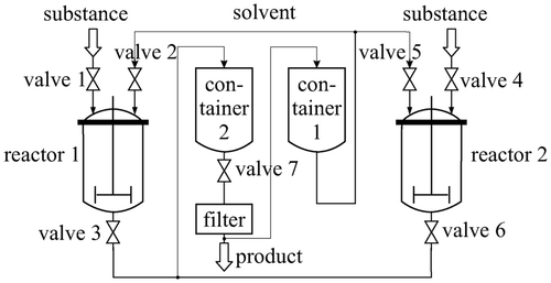
The final product of the batch process in figure 10 results from a reaction where a substance and a solvent are involved. In each batch cycle, defined quantities of substance and solvent are filled through the inlet valves 1, 4 and 2, 5, respectively, in the reactors 1 and 2. After the completion of both inlet processes for each reactor, a reaction takes place, the result of which flows through the valves 3 and 6 into the container 2. Then, the solvent is separated from the final product by a filter and collected in the container 1. As soon as this operation is completed the solvent is available for a new batch cycle. This behaviour is enforced by the PLC that opens and closes the valves 1,…, 7 issuing the binary signals V ₁,…, V ₇.

Overall system model

For the upper process hierarchy, the sequence of processing steps of the batch process is modelled by the timed event graph given in figure 11. The holding times τ _ij represent the durations of the inlet and outlet processes through the seven valves. The measured event times x_i (i = 1,…, 10) and the input event times u_j (j = 1, 2) correspond to the transitions q_i and input transitions of the timed event graph and are explained in detail in table 1.

Figure 11 Timed event graph representing the overall behaviour of the batch process. All places where no holding time is displayed have the holding time 0.

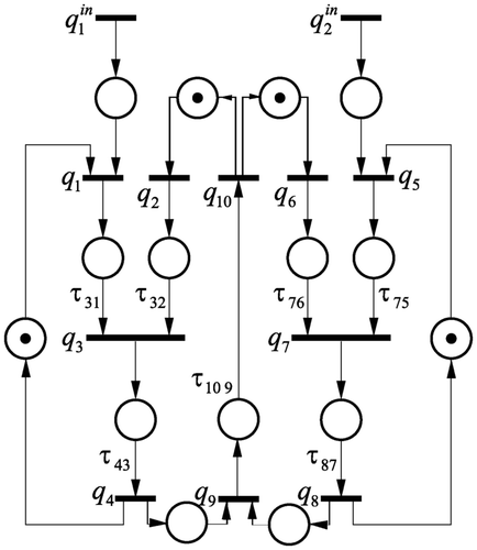
Table 1. System parameters and elements of the timed event graph

Event and corresponding changes in Vi	Transition
New charge of substance becomes available for reactor 1 | 2
Open valve 1 | 2 (Change V 1 | V 2 from 1 to 0)	q 1  |  q 2
Open valve 4 | 5 (Change V 4 | V 5 from 1 to 0)	q 5 | q 6
Close valves (1,2) | (4,5) and start reaction in reactor 1 | 2 (Change (V 1,V 2) | (V 4,V 5) from 0 to 1)	q 3 | q 7
Reactor 1 | 2 gets empty, close valve 3 | 6 (Change V 3 | V 6 from 0 to 1)	q 4 | q 8
Open valve 7 and start filtering (Change V 7 from 1 to 0)	q 9
Solvent becomes available, close valve 7 (Change V 7 from 0 to 1)	q 10
Process	Holding time	Corresponding valve
Fill substance into reactor 1 | 2	τ31 | τ75	valve 1 | 4
Fill solvent into reactor 1 | 2	τ32 | τ76	valve 2 | 5
React and empty reactor 1 | 2	τ43 | τ87	valve 3 | 6
Filter	τ10 9	valve 7

Based on the given timed event graph, the non-recursive equation that relates the event times to the processing times is determined

corresponding to Equation (6).

Component models for the valves

Each of the inlet and outlet valves of the containers and reactors has the structure shown in figure 12. Although each valve was considered from the overall system point of view as a switch that allows or prevents flows into or out of a reactor, a more detailed analysis on the component level shows that they consist of the following components 23:

	Control valve is the main part for controlling the fluid flow.
	Spring and diaphragm pneumatic servomotor is intended to provide a linear motion to servomotor stem.
	Positioner is a device applied to eliminate the control valve stem mispositions.

Figure 12 Schematic structure of a valve.

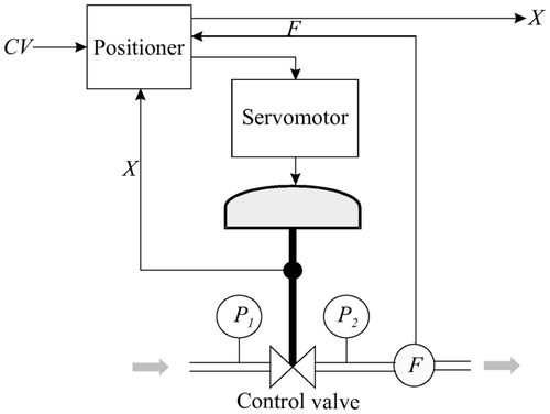
Each valve i receives a binary input variable CV = V_i from the PLC. The maximum and minimum values of CV correspond to the maximum and minimum movement of the piston rod, or the minimum and maximum flow rate, respectively.

The output measured by the sensors in each valve are the medium flow rate F and the piston rod displacement X. Additional measurable parameters are the upstream pressure and downstream pressure (P1 and P2) which are used to monitor the flow rate sensor. These data are not available at the overall system level because they are not transmitted to the PLC, but they are available to the diagnoser for component diagnosis upon request.

In the sequel three types of faults are considered for each valve:

1. f = 1: valve clogging,

2. f = 2: servomotor diaphragm perforation,

3. f = 3: leakage in the control valve.

The timed automaton representing the valves is obtained by the identification algorithm described in 15. The automaton consists of 432 states and approximately 15,000 transitions which cover the wide range of operating conditions for the actuator.

Hierarchical diagnosis

Figures 13 and 15 illustrate the diagnostic results. In figure 13 the grey box marks the region in which |r ₃₁/τ_31,Ref |<δ₃₁/τ_31,Ref holds. The persistent excitation was designed following the principles given in 18 and implemented in the PLC. The number of cycles used for parameter estimation by (21) and residual generation was set to N = 2.

Figure 13 Event sequences used at the upper process level.

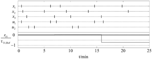
The ticks in the upper part of figure 13 denote the occurrence times of the process events that correspond to transition firing times of the timed event graph. At time t = 605 seconds valve 1 clogs at 50% of the normal valve stroke during the valve closing process in cycle k + 1. Note that for the computation of the residual r ₃₁ only the firing times x ₁ and x ₃ of the transitions q ₁ and q ₃ are required. After the measurement of x ₁(k + 2) = m ₁(k + 2) and x ₃(k + 2) the residual r ₃₁ significantly deviates from zero (see the lower part of figure 13) indicating that some fault affects the substance inlet process in reactor 1. As the valve 1 is the only component involved in the execution of this process, the hierarchical diagnostic algorithm activates the component diagnosis for valve 1.

The diagnosis of the valve 1 starts with reading the data of the last two process cycles from the data archive. Figure 14 shows the discrete data of the valve retrieved for diagnosis. The bars in the figure denote the discrete values of each signal. It can be seen that the data is retrieved from the buffer starting from the time when the valve 1 started to open as shown by the decrease of the rod displacement X.

Figure 14 Signals retrieved for diagnosis from the archive starting at t = 8 minutes.

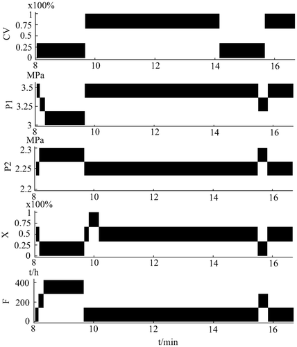
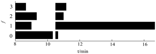
The diagnostic result of valve 1 is shown in figure 15. The horizontal bar in the figure denotes the time horizon until which the archived discrete inputs and outputs are consistent with the model for respective fault. The diagnostic algorithm is started with the data beginning at t = 8 minutes in order to determine the occurrence time of the fault which has been detected around t = 15.5 minutes by means of parameter estimation. For the first 2 minutes of the diagnosis of valve 1, the algorithm finds that there is actually no fault in this component as denoted by the consistency of f ₀ in figure 15. However, once the fault occurs at 605 seconds, the timed automaton representing the faultless system becomes inconsistent with the measurement, which proves the existence of a fault in this valve. Hence, the valve is isolated as a faulty component. Algorithm 2 is then reinitialized and after a short time the fault f ₁ (Valve clogging) is identified.

Figure 15 Diagnostic results from lower process hierarchy.

In principle, the timed automaton alone could be used for fault detection and isolation. However, the modelling complexity for the overall system using a single timed automaton would be very high and make on-line diagnosis impossible. Note that it is well known that the modelling effort and the complexity of the model grow faster than the size of the process. This example illustrates that by decomposing the process into two model forms which are used together by exploiting the process hierarchy one can use the advantages provided by each method.

7 Conclusion

This paper has presented a new method for diagnosing discrete-event systems with a hierarchical structure. The diagnosis is based on two model-based diagnostic methods that use timed discrete-event representations. The two models separate the global and local behaviour of the process and reduce the complexity of the diagnostic task. The timed event graph as a coarser model is used to represent the overall process, which has a predetermined sequential operation. The diagnosis at this process layer is done by parameter estimation. The timed automaton which contains more detailed information is used to represent individual process components. Once the existence of a fault has been detected on the higher level and associated with some components, the diagnosis at the lower process level starts for fault isolation and identification. The principle and performance of the proposed diagnostic method was illustrated by diagnosing actuator faults in a batch process.

The field of application of the presented method covers complex systems for which the temporal distance between events is influenced by the presence of faults and, from a detailed view point, the behaviour of the components may be given by non-deterministic event sequences. Fault diagnosis of such systems necessitates to use timed models like timed event graphs or timed automata. Furthermore, the methods developed here are applicable under real-time constraints because the given algorithms process only a small amount of data with simple operations in each cycle.

Acknowledgements

This project has been supported by the Deutsche Forschungsgemeinschaft under grants Kr 949/9 and Lu 462/13.

Notes

¹This means that the first firing of e.g. the transition q_i can occur only after the first firing of the transition . The assumption is for convenience only. The extension is straightforward.

References

- Blanke , M. , Kinnaert , M. , Lunze , J. and Staroswiecki , M. 2003 . Diagnosis and fault-tolerant control , Berlin : Springer-Verlag .
- Sampath , M. , Sengupta , R. , Lafortune , S. , Sinnamohideen , K. and Teneketzis , D. C. 1996 . Failure diagnosis using discrete-event models . IEEE Transactions on Control Systems Technology , 4 : 105 – 124 .
- Hashtrudi Zad , S. , Kwong , R. H. and Wonham , W. M. . Fault diagnosis in timed discrete-event systems . In Proc. 38th IEEE Conference on Decision and Control . 7 – 10 December 1999 . pp. 1756 – 1761 . Phoenix
- Pandalai , D. N. and Holloway , L. E. 2000 . Template languages for fault monitoring of timed discrete event processes . IEEE Transactions on Automatic Control , 45 : 86 – 882 .
- Srinivasan , V. S. and Jafari , M. A. 1993 . Fault detection/monitoring using time petri nets . IEEE Transactions on Systems, Man and Cybernetics , 23 : 1155 – 1162 .
- Lunze , J. 2000 . Diagnosis of quantized systems based on a timed discrete-event model . IEEE Transactions on Systems, Man and Cybernetics, Part A , 30 : 322 – 335 .
- Mozetic , I. 1991 . Hierarchical model-based diagnosis . International Journal of Man-Machine Studies , 35 : 329 – 362 .
- Baroni , P. , Lamperti , G. , Pogliano , P. and Zanella , M. 2000 . Diagnosis of a class of distributed discrete-event systems . IEEE Transactions on Systems, Man and Cybernetics, Part A , 30 : 731 – 752 .
- Lamperti , G. and Zanella , M. 2003 . “ Diagnosis of active systems, principles and techniques ” . In Kluwer International Series on Engineering and Computer Science , Vol. 741 , Dordrecht : Kluwer Academic .
- Debouk , R. , Lafortune , S. and Teneketzis , D. C. 2000 . Coordinated decentralized protocols for failure diagnosis of discrete event systems . Discrete Event Dynam. Syst. , 10 : 33 – 86 .
- Cassandras , C. and Lafortune , S. 1999 . Introduction to Discrete Event Systems , Boston : Kluwer Academic .
- Baccelli , F. , Cohen , G. , Olsder , G. J. and Quadrat , J. -P. 1992 . Synchronization and Linearity , Chichester : John Wiley .
- Cuninghame-Green , R. 1979 . Minimax algebra, volume 166 of Lecture Notes in Economics and Mathematical Systems , Berlin : Springer-Verlag .
- Alur , R. and Dill , D. 1994 . A theory of timed automata . Theoretical Computational Science , 126 : 183 – 235 .
- Supavatanakul , P. , Falkenberg , C. and Lunze , J. . Identification of timed discrete-event model for diagnosis . In Proc. 14th International Workshop on Principles of Diagnosis . 11 – 14 June 2003 , Washington, DC.
- Schullerus , G. and Krebs , V. . Diagnosis of batch processes based on parameter estimation of discrete event models . In Proc. 6th European Control Conference . 4 – 7 September 2001 , Porto. pp. 1612 – 1617 .
- Menguy , E. , Boimond , J. -L. , Hardouin , L. and Ferrier , J. L. 2000 . A first step towards adaptive control for linear systems in max algebra . Discrete Event Dynamic Systems , 10 : 347 – 368 .
- Schullerus , G. 2004 . Identifikation Zeitbewerteter Ereignisdiskreter System , Düsseldorf : VDI Verlag . VDI Fortschritt-Berichte, Vol. 8
- Lunze , J. and Supavatanakul , P. . Diagnosis of discrete-event systems described by timed automata . In Proc. IFAC World Congress . 21 – 26 July 2002 , Barcelona.
- Supavatanakul , P. 2004 . Modelling and diagnosis of timed discrete-event systems Steuerungs- und Regelungstechnik , Aachen : Shaker Verlag .
- Lunze , J. 1995 . Künstliche Intelligenz für Ingenieure , 2nd edition , München : Oldenbourg Verlag .
- Hanisch , H. -M. 1992 . Petri-Netze in der Verfahrenstechnik , München : Oldenbourg Verlag .
- Bartys , M. 2002 . “ Specification of the actuators intended to use for benchmark definition ” . Available online at: http://diag.mchtr.pw.edu.pl/damadics (accessed 18 April 2006)