Comparison of discretization methods to solve a population balance model of activated sludge flocculation including aggregation and breakage

Abstract

Population balance models (PBMs) can be used to describe the evolution with time of distributions of properties of individuals. In this study a PBM for activated sludge flocculation including aggregation and breakage processes was investigated. The PBM is an integro-differential equation and does not have an analytical solution. A possibe method of solving the equation at relatively low computational cost is to use discretization. Two different discretization techniques, the fixed pivot and the moving pivot, were compared using geometric grids of different coarseness. Simulations were performed for three different processes: pure aggregation, pure breakage and combined aggregation – breakage. The results for pure aggregation showed that the fixed pivot overpredicts the large particle sizes when using coarse grids since grid refinement results in a clear downward trend. The predictions of the moving pivot technique show even lower predictions for the large particle sizes, with a slight upward trend for finer grids. This suggests that these predictions are closer to the pseudo-analytical solution (i.e. at infinitely fine grid). For the pure breakage case it was found that the moving pivot predictions collapsed onto one curve. Since a binary breakage case was studied, a fixed pivot with a grid with geometric factor 2 also collapsed onto that curve. Grid refinement for the fixed pivot case resulted in overestimations. Similar conclusions could be drawn for the combined aggregation – breakage case. Overall, the moving pivot is found to be superior since it produces more accurate predictions, even for much coarser grids. Despite the computational burden, the latter implies a lower computational load.

Keywords:

• Population balance model
• Discretization
• Aggregation
• Breakage

1. Introduction

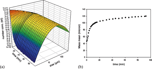
A population balance model (PBM) can be used to describe the time evolution of one or more property distributions of individuals of a population. This type of model was proposed in the late 1970s 1, but applications were limited because of a lack of computational power and appropriate measurement techniques to feed the models. Since these limitations have gradually eased over recent decades, the popularity of PBMs has increased which is reflected by an increase in the number of studies using this type of model. Applications can be found in various scientific fields dealing with a ‘population’ of individuals, such as crystallization, flocculation, flotation, polymerization, precipitation, aerosol dynamics, cell age evolution, etc. Typically, one is interested in describing the evolution of the distribution of a population property (e.g. size, specific surface area, fractal dimension, density, cell age, cell storage material). The aim is either to improve understanding of certain phenomena or to predict the evolution of the distribution in order to control certain processes. An example of the type of experimental data that can be described by a PBM (taken from a biological flocculation experiment using activated sludge 2) is shown in figure 1. It shows the evolution of a number distribution in time, together with the evolution of the mass mean diameter of the distribution which is often used as a summarizing parameter.

Figure 1. Example of the type of data that can be modelled using a PBM: evolution with time of (a) size distribution and (b) the mass mean derived from the distributions 2.

The format of the PBM depends on the process under study. The most general (multidimensional) format of the population balance equation is as follows 3:

where x is a vector of properties, f(x,t) is the joint property distribution function, [Xdot] is a vector containing the time derivatives of x, ▿ _x is the gradient operator (i.e. the sum of all partial derivatives of the scalar on which it operates with respect to the elements of the vector x), and h(x,t) represents the birth and death of individuals typically occurring through aggregation and breakage. In the following sections the structure of the model is described, two methods for solving this type of equation using discretization are presented, and simulations using these two solution techniques are compared.

2 Description of the model

In the application investigated in this paper, activated sludge flocculation, the individuals are activated sludge flocs, the property vector x is the floc size (one-dimensional PBM) expressed as volume, and the distribution f(x,t) is the number distribution. Since the model will be used to describe data from relatively short flocculation experiments, biological floc growth is not considered. Therefore the second term in equation (1) disappears because [Xdot] is zero. The function h(x,t) consists of birth and death terms for both aggregation and breakage. Note that this function typically consists of four terms, two for aggregation (birth and death) and two for breakage (birth and death).

Most aggregation models are based on the ‘integral’ Smoluchowski equation 4:

where α is the collision efficiency and β is the aggregation frequency function, often referred to as the ‘aggregation kernel’.

The first term on the right-hand side of equation (2) describes the increase in flocs of size x by aggregation of two smaller flocs (x–x′ and x′) whose total volume is equal to the volume of a floc of size x (aggregation birth). The second term on the right-hand side of equation (2) describes the loss of flocs of size x because of their aggregation with flocs of any other size (aggregation death).

In a PBM describing flocculation, the aggregation kernel β represents the number of collisions that occur and can be interpreted as a description of the transport of the particles towards each other. Typically, the aggregation kernel is a function of the volume of the colliding particles. The aggregation kernel used in this study is a ‘sum kernel’ (since it is a function of the sum of the particle volumes) and is expressed as follows 5:

where G is the average velocity gradient and v _i is the volume of particle i. It describes orthokinetic flocculation caused by fluid shear. Other methods of particle transport can occur, such as Brownian motion (perikinetic flocculation) or differential sedimentation. However, these are not considered here.

The factor α represents the fraction of collisions that are successful. It corrects for hydrodynamic and/or electrostatic interactions which might affect the success of a collision. It is often chosen to be a constant (fitting parameter) but it can be dependent on particle properties (e.g. size) 6.

Breakage models are typically expressed as follows:

where n(x) is the average number of daughter particles that are formed per breakage event, Γ is the daughter distribution function, which describes the properties of the particles that are formed, and S is the breakage rate or ‘breakage kernel’. The first term on the right-hand side of equation (4) describes the increase in the number of flocs of size x as a result of break-up of larger flocs (breakage birth). The second term on the right-hand side of equation (4) describes the loss of flocs of size x because of breakage (breakage death). In the literature, binary breakage is often assumed, i.e. n(x) = 2. The daughter distribution function can be a discrete or a continuous function. In this study it is assumed that particles break up into two daughter particles with equal volumes. The breakage kernel is function of the particle volume. Some studies relate the breakage kernel to the turbulence regime, leading to complex functionals 7,8. The following breakage kernel was chosen in this simulation study 9:

where A is the breakage rate and a is a constant which is chosen to be 1/3. The latter implies a linear relationship with the floc diameter.

Combining equations (1) –  (5) results in an integro-differential equation which, depending on the aggregation and breakage functions used, rarely has an analytical solution. Hence other techniques, such as successive approximation, Laplace transforms, weighted residuals, discretization, or Monte Carlo simulation, are used to solve the equation. An overview of the different techniques used to obtain approximate solutions for PBMs can be found in 3. In this simulation study we use discretization techniques to solve the population balance model.

When the property vector x is discretized, the integrals in equations (2) and (4) become summations and the integro-differential equation is converted into a set of ordinary differential equations which can be solved simultaneously using a time-integration algorithm. However, accurate solutions need a fine grid which implies a high computational load. If an accurate solution of the complete distribution is needed, it is necessary to use a fine grid and the coarseness will determine the accuracy of the solution. If accurate estimates of certain properties of the distribution are required, it is possible to use other techniques 10,11 which were developed in order to decrease the computational load while still ensuring the conservation of at least two integral properties of x (e.g. numbers and mass). These techniques will be discussed in more detail in the following sections.

3 The fixed pivot approach

Several authors have proposed methods of solving a population balance equation numerically using a reduced number of equations by applying discretization. The reduction in the number of equations implies that the accuracy of the solution deteriorates. However, in some cases one is not interested in an accurate solution of the complete distribution, but only the conservation of certain properties (e.g. number or mass conservation). Batterham et al. 12 used a geometric grid (v _i+1 = 2v _i , where v is the floc volume) to solve a pure aggregation population balance model conserving mass only. Hounslow et al. 13 used a similar grid and developed a set of equations conserving both number and mass for pure aggregation systems. Litster et al. 14 generalized Hounslow's technique for other geometric grids (v _i+1 = rv _i , where r = 1/q and q is a positive integer), again for pure aggregation. Finally, Hill and Ng 15 developed a similar technique for pure breakage problems. The main disadvantage of these methods is that they can only be used for one or a limited number of geometric grids and that the conservation of distribution properties is restricted to number and mass. When another grid is to be used and the properties of interest are different, new equations need to be derived.

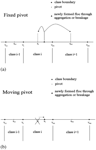
In order to solve this problem, Kumar and Ramkrishna 10 proposed a framework which allowed conservation of any two chosen integral properties of the distribution. Moreover, the numerical technique developed can be used for any arbitrarily chosen grid. The main difficulty which needs to be overcome is that particles can be formed (through either aggregation or breakage) whose property x does not coincide with one of the existing grid points or ‘pivots’. Two property balances are used to reallocate these particles to the adjoining pivots ( figure 2(a)). Thus two arbitrarily chosen properties of the distribution can be conserved.

Figure 2. Schematic representation of how the different techniques deal with newly formed particles which do not coincide with an existing pivot: (a) fixed pivot; (b) moving pivot.

The set of equations needed to conserve both mass and number is as follows 10:

where

where Γ(v,x _k ) is the breakage distribution function, i.e. the probability that a daughter particle of size v is formed from the breakage of a particle of size x _k . In this study, Γ(v,x _k ) was chosen to be 1 if v = x _k /2 and zero in all other cases.

Equation (6) consists of four terms. The first is the aggregation birth term and contains a factor η (defined in equation (7)) responsible for the reallocation of the particles formed to the adjoining pivots if they do not coincide with a pivot. If they do coincide with a pivot, η = 1. It is important to note here that the summation is performed for aggregated particles which have a volume between the pivots x _i−1 and x _i+1. The second term describes the loss of particles due to aggregation (aggregation death) and does not require any reallocation since particles only disappear and are not formed. the third term (breakage birth) requires a factor for reallocation (n _i,k ) based on the breakage distribution function (equation (7)). The fourth term describes the loss of particles due to break-up (breakage death), and since no particles are formed during this process this term does not require any reallocation. Note that equations (6) and (7) are simplified equations which can only be used to conserve number and mass; hence they yield identical results to the equations derived by Hounslow et al. 13 when a geometrical grid with factor 2 (volume-based) is used. The advantage of the fixed pivot technique is its generality in terms of the properties to be conserved and the grid choice. The general equations of the fixed pivot technique can be found in the literature 2,10.

Kumar and Ramkrishna 10 compared their technique with an analytical solution (i.e. their population balance model had a rather simple structure with regard to aggregation and breakage kernels) to check the performance of the technique for pure break-up, pure aggregation, and combined aggregation – breakage. The technique produced accurate predictions for pure break-up even when coarse grids were used. The cases involving aggregation (pure aggregation and the combined case) suffered from severe overprediction at large particle sizes. The degree of overprediction was reduced by using a finer grid. The overprediction was attributed to steep non-linear gradients in the number density functions. This problem was addressed by the moving pivot technique described in the next section.

4 The moving pivot approach

In order to overcome the problem of steep non-linear gradients in the number density functions, leading to overprediction in the large particle size range, Kumar and Ramkrishna 11 proposed the ‘moving pivot’ technique. This technique accounts for the evolving non-uniformity of the distribution in each interval as a result of breakage and aggregation events by allowing a varying pivot location ( figure 2(b)). The other features (arbitrary choice of grid and integral properties to be conserved) were maintained. Details of the derivation of the equations can be found in the literature 2,11. The equations conserving number and mass are as follows:

where

The first expression in equation (8) describes the time variation of N _i and looks similar to that in the fixed pivot method. It also contains four terms (aggregation birth/death and breakage birth/death). However, the first and third terms are different from those in equation (6). The difference in the first term is the fact that the summation now involves aggregated particles which are formed between the class boundaries v _i and v _i+1 (and not between pivots as was the case in the fixed pivot approach). A similar difference occurs in the third term where the integrals (equation (9)) have different limits from those for n _i,k (equation (7)). A closer look at the second expression in equation (8) reveals that only two terms are responsible for changing the pivots x _i , one for aggregation birth and one for breakage birth. In fact, the equation is just a determination of the average diameter (in this case volume) of every size class when new particles are created in them. In this way, the pivots are allowed to move inside the class boundaries depending on the number and volume of particles that are created in the class through either aggregation or breakage.

The moving pivot technique was compared with the fixed pivot technique, but only with respect to its additional features 11. It was found that it did not overpredict in the large particle size range; rather, a small underprediction was observed. However, the results for the moving pivot technique were much closer to the analytical solution than those obtained using the fixed pivot technique with exactly the same grid. Further refinement of the grid improved the accuracy of the solution.

5 Numerical results

The aim of this study was to compare solutions of the PBM described in section 2 and to determine the optimal solution method and grid coarseness, taking into account both the accuracy of the solution and the required calculation time. Three cases were investigated: pure aggregation, pure breakage, and combined aggregation – breakage. Unlike the investigations by Kumar and Ramkrishna 10 11, no analytical solution of the PBE was available. The solution methods described in sections 3 and 4 were implemented in the modelling and in the simulation platform WEST (Hemmis NV, Belgium) which was used to perform all simulations 16.

5.1 Simulation conditions

The distribution properties to be conserved were chosen to be number and mass (zeroth and third integral moments of the number distribution). Different geometrical grids were used (v _i+1 = sv _i , 1.1 ≤ s ≤ 2). The lower boundary of the size range was chosen to be 0.6 μm because the single bacterial cells making up the floc have a diameter of about 1 μm. The upper boundary of the size range was chosen to be the upper limit of the class for which the pivot did not exceed 800 μm. Thus the number of classes ranged from 31 for the case where s = 2 to 226 for the case where s = 1.1. A floc monodispersion of diameter 5.5 μm with a total volume of 5.9 × 10¹⁰μm³ was chosen as the initial condition. The average velocity gradient G was chosen to be 37.0 s⁻¹.

The initial conditions were calculated for each of the different grid – solution method combinations. When using the fixed pivot technique, the pivots between which the monodisperse diameter was situated were identified, and the mass and number were reallocated to the adjoining pivots conserving both mass and number of the monodispersion (same procedure as described for the fixed pivot (see section 3)). All other N _i values were set to zero. When using the moving pivot technique, the class containing the monodisperse diameter was assigned a pivotal size of 5.5 μm and was filled with 6.77 × 10⁸ flocs as the initial N _i . All other pivots were chosen to be class centres and the N _i values were set equal to 10⁻¹³. This is needed because equation (8) contains a division by N _i . The value was chosen such that no mass is added to the system. Parameters α and A were set at 0.1 and 5000, respectively (or to zero for the pure aggregation and pure breakage cases), which corresponds to moderate aggregation and breakage. In order to check for mass losses the third moment of the distribution was monitored during all simulations. No significant mass losses were observed in any of the simulations (<10⁻³%).

The numerical results are presented in terms of cumulative oversize number (CON) as a function of the floc volume, which is defined as follows:

This plot emphasizes the predictions for number density in the large particle size tail of the distribution and the zeroth moment of the size distribution (total number) in a single plot. To emphasize the predictions in the small particle size tail, the cumulative undersize number (CUN) can be used, which is similar to CON except that it has different integration limits:

5.2 Pure aggregation and pure breakage simulations

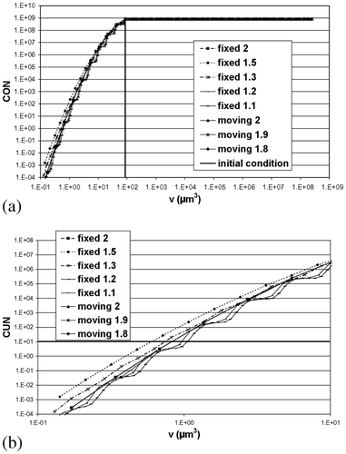
First, simulations using either the fixed or the moving pivot approach were performed for the pure aggregation and pure breakage processes. The results are shown in figure 3 for pure aggregation (A = 0) at t = 23 s and in figure 4 for pure breakage (α = 0) at t = 10 s. These time points were chosen so that it was possible to observe the moving front. Since a steady state will not be reached for pure aggregation and pure breakage, the front eventually disappears after a while and the volume becomes concentrated in the largest size class for pure aggregation and in the smallest size class for pure breakage.

Figure 3. Prediction of the cumulative oversize number (CON) as a function of the particle volume for pure aggregation (A = 0) at t = 23 s: (a) complete range, (b) enlarged section.

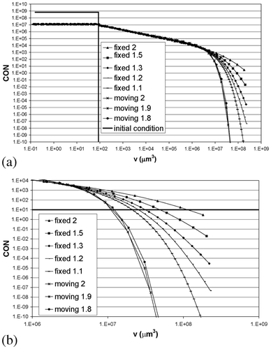
Figure 4. Prediction of the cumulative undersize number (CUN) as a function of the particle volume for pure breakage (α = 0) at t = 10 s: (a) complete range; (b) enlarged section.

For pure aggregation, five different geometric grids were studied using the fixed pivot method (s values of 1.1, 1.2, 1.3, 1.5, and 2) and three using the moving pivot technique (s values of 2, 1.9, and 1.8). Coarse grids tend to overpredict the large particle sizes for the fixed pivot technique and hence inherently overpredict the rate of aggregation. This can clearly be seen in figure 3(b) where grid refinement results in lower predictions for the CON tail. The improvements in accuracy for the grids investigated was evaluated at CON = 10 (i.e. the volume at which there are still 10 oversized particles). These improvements are still quite large in the fixed grids, implying that even the accuracy of the finest grid (s = 1.1) is not very great. This can be seen in table 1 which summarizes the corresponding diameters for CON = 10. Litster et al. 14 used s values as low as 1.12 to approach an analytical solution for their case. As the results here show, this still seems to be too coarse.

Table 1. Diameters corresponding to CON = 10 for the pure aggregation case using different solution techniques (at t = 23 s).

Solution technique and grid coarseness	Diameter (μm)
Fixed pivot, s = 2.0	641
Fixed pivot, s = 1.5	466
Fixed pivot, s = 1.3	396
Fixed pivot, s = 1.2	365
Fixed pivot, s = 1.1	343
Moving pivot, s = 2.0	319
Moving pivot, s = 1.9	301
Moving pivot, s = 1.8	330

The moving pivot technique resulted in even smaller numbers of large particles compared with the fixed pivot predictions. When refining the grid, rather higher predictions of the CON tail are observed. However, the improvements in accuracy between the grids investigated at CON = 10 are much smaller, implying that the accuracy cannot be improved much by further refining the grid. Moreover, in view of the convergence of the fixed pivot predictions and the relative stability of the moving pivot predictions, the solution obtained using the latter can be regarded as being close to the pseudo-analytical solution. This is confirmed in table 1 as the increase in diameter when refining the grid with the moving pivot is less than the decrease was observed with the fixed pivot. This was also noted by Kumar and Ramkrishna 11. They compared the results with the analytical solution and found that the latter lay between the fixed and moving pivot predictions, but closer to the latter. It can be concluded that the moving pivot technique is superior in terms of accuracy, even for coarse grids. However, it should be noted that the calculation load for the moving pivot is higher than that for the fixed pivot for the same grid coarseness. It is recommended that the moving pivot technique is used for pure aggregation cases since coarser grids, which are less computation intensive than the fine grids required by the fixed pivot, can be used to obtain the same accuracy.

For pure breakage, five grids were studied using the fixed pivot method (s values of 1.1, 1.2, 1.3, 1.5, and 2) and three using the moving pivot technique (s values of 2, 1.9, and 1.8). For the different moving pivot grids, the predictions almost completely collapse onto the same curve and the pivots, although starting at a different value for each grid at t = 0 s, all move to the pivot values of the grid with s = 2. Moreover, the prediction of the fixed grid for s = 2 collapses onto the same curve. For finer grids, the fixed pivot yielded different results at CUN = 10 ( table 2). This rather surprising result actually has a simple explanation. It is caused by the kind of breakage used in this study (binary breakage into equally sized daughters). If a grid with s = 2 is used, a breakage event will produce particles which are the size as the pivot of the underlying class. Therefore no errors will be made when this kind of grid is used, and the fixed and moving pivot techniques will yield the same result. However, when a finer grid is used, the fixed pivot method is unable to correct for the fact that particles are created in volumes different from the pivot. The moving pivot can correct for this by moving to the same volumes as for a grid with s = 2 (still remaining within their boundaries). This example shows the flexibility of the moving pivot technique. When even finer grids are used for the fixed pivot (s values of 1.1 and 1.2), waves start to build up in the solution. This is also due to the binary breakage into equal-sized daughters. Some classes of particles simply cannot be formed. Grid refinement does not appear to give a more accurate solution in the breakage case. Only the fixed pivot case with s = 2.0 yields comparable results to those obtained with the moving pivot. However, it should be noted that, for other kinds of breakage (e.g. binary breakage into unequal daughters, multiple breakage), the comparison between the two solution methods is expected to be similar to the results obtained for aggregation, i.e. the moving pivot will be superior. Therefore it is recommended that the moving pivot is used for pure breakage.

Table 2. Diameters corresponding to CON = 10 for the pure breakage case using different solution techniques (at t = 10 s).

Solution technique and grid coarseness	Diameter (μm)
Fixed pivot, s = 2.0	1.10
Fixed pivot, s = 1.5	1.01
Fixed pivot, s = 1.3	1.10
Fixed pivot, s = 1.2	1.22
Fixed pivot, s = 1.1	1.25
Moving pivot, s = 2.0	1.10
Moving pivot, s = 1.9	1.10
Moving pivot, s = 1.8	1.10

5.3 Combined aggregation – breakage simulations

Finally, the PBM was solved for the combined aggregation – breakage case. Under the conditions mentioned above, it takes about 300 s to reach a steady-state particle size distribution. The steady-state numerical results for CON and CUN are shown in figures 5 and 6, respectively. Again, five grids were studied using the fixed pivot method (s values of 1.1, 1.2, 1.3, 1.5, and 2) and three using the moving pivot technique (s values of 2, 1.9, and 1.8). For the fixed pivot approach, the CON tail predictions are different for the grids investigated with a clear direction of change. A similar, but less pronounced, effect to that in the pure aggregation case is observed. The diameter values obtained at CON = 10 are summarized in table 3. A downward trend can clearly be observed and it is assumed that the ‘exact’ or pseudo-analytical solution can be found by further refinement of the grid. A similar trend has been observed by other researchers 10,14.

Figure 5. Steady-state prediction of the cumulative oversize number (CON) as a function of the particle volume for the fixed and moving pivot: (a) complete range; (b) enlarged section.

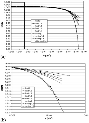
Figure 6. Steady-state prediction of the cumulative undersize number (CUN) as a function of the particle volume for the fixed and moving pivot: (a) complete range; (b) enlarged section.

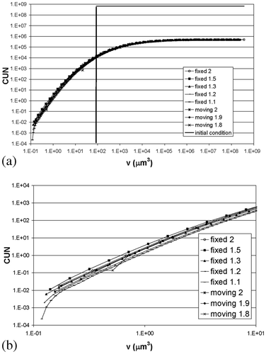
Table 3. Diameters corresponding to CON = 10 and CUN = 10 for the combined aggregation – breakage case using different solution techniques (at t = 10 s).

Solution technique and grid coarseness	Diameter (μm)
	CON = 10	CUN = 10
Fixed pivot, s = 2.0	441	1.43
Fixed pivot, s = 1.5	406	1.40
Fixed pivot, s = 1.3	369	1.50
Fixed pivot, s = 1.2	356	1.56
Fixed pivot, s = 1.1	343	1.59
Moving pivot, s = 2.0	337	1.45
Moving pivot, s = 1.9	334	1.47
Moving pivot, s = 1.8	346	1.45

Since the difference between the grids with s values of 1.2 and 1.1 is still rather large, it is thought that the accuracy is still not very high and that further grid refinement is necessary. Again, the moving pivot predictions for large particle sizes are much lower than the fixed pivot solution. Since grid refinement does not result in large differences (<2%), the moving pivot can be considered to be closer to the pseudo-analytical solution and hence is superior to the fixed pivot.

The predictions for smaller particle sizes ( figure 6) are also different for the investigated grids. Similar results to those for the pure breakage case were found. However, the moving pivot predictions do not collapse as perfectly onto the same curve for all grids (again the curve obtained with the fixed pivot for s = 2) as was the case in the pure breakage case. Further refining the grid in the fixed pivot case leads to lower predictions of the CUN tail. This is probably because of inaccuracies introduced by the aggregation. Therefore in this case it is less clear that the moving pivot is superior and will produce more accurate results. However, based on the CON values, the moving pivot is still thought to be superior.

Overall, it can be concluded that the moving pivot approach is superior to the fixed pivot method, even for coarse grids (s = 2). Therefore more accurate predictions than those obtained using the fixed pivot approach can be obtained at much lower computational cost (coarser grids can be used).

6 Summary

Two different methods of solving a PBM for activated sludge floccuation using discretization, the fixed pivot and the moving pivot techniques, have been presented. Simulations for geometric grids with different coarseness using both techniques were compared for three different processes: pure aggregation, pure breakage, and combined aggregation – breakage. The pure aggregation case revealed that the fixed pivot technique overpredicts the CON tail (i.e. the number of large particles) when using coarse grids. The moving pivot technique yielded much lower predictions, but since grid refinement caused only minor changes, it is, in agreement with literature reports, thought to be more accurate than the fixed pivot technique (even for coarse grids). In the pure breakage case, the fixed pivot technique with a grid with a geometric factor of 2 was found to produce accurate results for the specific breakage case investigated (binary breakage into equally sized daughters). This will not be true for more general breakage cases, and the moving pivot is again expected to be superior. The combined aggregation – breakage case revealed very similar results to the pure cases. Overall, the moving pivot is found to be superior in almost all cases investigated. The only drawback of this method is its larger computational cost per size class considered. However, this is more than compensated by its numerical efficiency, since significantly coarser grids yield more accurate results than with the fixed pivot approach.

Acknowledgements

This research was financially supported by the Fund for Scientific Research – Flanders (project G.0032.00) and the Ghent University Research Fund (BOF 01111001).

References

- Ramkrishna , D. 1979 . Statistical models of cell populations . Advances in Biochemical Engineering , 11 : 1 – 47 .
- Nopens , I. , Biggs , C. , De Clercq , B. , Govoreanu , R. , Wilen , B. , Lant , P. and Vanrolleghem , P. 2001 . Modelling the activated sludge flocculation process combining laser light diffraction particle sizing and population balance modelling (PBM) . Water Science and Technology , 45 : 41 – 49 .
- Ramkrishna , D. 2000 . Population Balances: Theory and Applications to Particulate Systems In Engineering , New York : Academic Press .
- Thomas , D. N. , Judd , S. J. and Fawcett , N. 1999 . Flocculation modelling: a review . Water Research , 33 : 1579 – 1592 .
- Spicer , P. T. and Pratsinis , S. E. 1996 . Shear-induced flocculation: the evolution of floc structure and the shape of the size distribution at steady state . Water Research , 30 : 1049 – 1056 .
- Kusters , K. , Wijers , J. and Thoenes , D. 1997 . Aggregation kinetics of small particles in agitated vessels . Chemical Engineering Science , 52 : 107 – 121 .
- Ducoste , J. 2002 . A two-scale PBM for modeling turbulent flocculation in water treatment processes . Chemical Engineering Science , 57 : 2157 – 2168 .
- Maggioris , D. , Goulas , A. , Alexopoulos , A. , Chatzi , E. and Kiparissides , C. 2000 . Prediction of particle size distribution in suspension polymerisation reactors: effect of turbulence nonhomogeneity . Chemical Engineering Science , 55 : 4611 – 4627 .
- White , E. T. and Ilievsky , D. 1996 . “ The use of the population balance for modelling metallurgical systems ” . In Emerging Separation Technologies for Metals II , Edited by: Bautista , R. 91 – 103 . Warrendale, PA : Minerals, Metals and Materials Society .
- Kumar , S. and Ramkrishna , D. 1996 . On the solution of population balance equations by discretisation. I: A fixed pivot technique . Chemical Engineering Science , 51 : 1311 – 1332 .
- Kumar , S. and Ramkrishna , D. 1996 . On the solution of population balance equations by discretisation. II: A moving pivot technique . Chemical Engineering Science , 51 : 1333 – 1342 .
- Batterham , R. J. , Hall , J. S. and Barton , G. Pelletizing kinetics and simulation of full scale balling circuits . Proceedings of the 3rd International Symposium on Agglomeration, Nurnberg . pp. A136
- Hounslow , M. J. , Ryall , R. L. and Marshall , V. R. 1988 . A discretized population balance for nucleation, growth and aggregation . AIChE Journal , 34 : 1821 – 1832 .
- Litster , J. D. , Smit , D. J. and Hounslow , M. J. 1995 . Adjustable discretised population balance for growth and aggregation . AIChE Journal , 41 : 591 – 603 .
- Hill , P. and Ng , K. M. 1995 . New discretisation procedure for the breakage equation . AIChE Journal , 41 : 1204 – 1216 .
- Vanhooren , H. , Meirlaen , J. , Amerlinck , Y. , Claeys , F. , Vangheluwe , H. and Vanrolleghem , P. 2003 . WEST: Modelling biological wastewater treatment . Journal of Hydroinformatics , 5 : 27 – 50 .