Model order reduction for object-oriented models: a control systems perspective

Abstract

In recent years several concepts and tools for modelling and simulation of non-linear heterogeneous and multi-domain systems have been developed, speeding up to a great extent the process of an accurate analysis by simulation of increasingly complex technological systems. In parallel, for dimensioning and, above all, for control system design purposes, the need of models of reduced complexity has emerged; together with the need of tools capable of extracting, from the overall dynamic model, reduced models representing the dominant behaviour. This article reviews recent results in non-linear model order reduction method (NORM), originally developed with reference to computer-aided analysis and design of electronic circuits, and puts them in a control system design-oriented perspective, pointing out interesting future research directions.

Keywords:

• model order reduction
• object-oriented modelling
• control system design
• non-linear systems

1. Introduction

Equation-based, object-oriented modelling techniques, languages and tools emerged during the 1990s and are now well established in the modelling and simulation field, in particular to support the design of modern integrated systems, which require multi-physics modelling capabilities. Object-oriented models are usually non-linear, and mostly used for simulation purposes. There is a strong interest in object-oriented modelling for control system analysis and design, but so far the use of such models to support control-related activites has been mostly limited to the verification of the control system performance in closed loop by simulation, rather than giving direct support to the controller design [1]. For this specific purpose, the equations that correspond to object-oriented models built by the aggregation of reusable components are usually too complex, and not formulated in a way that can be directly used in the controller design.

In the field of electronic circuit analysis and design, a research interest has recently emerged in Model Order Reduction (MOR) techniques for non-linear circuits [2,3]. The main motivation behind this interest is to support hardware design activities. On one hand, as pointed out in Refs. [4] and [5], the design of modern mixed-signal (analog and digital) integrated circuits represents a challenge for modelling and simulation software, due to the ever-increasing complexity of the circuits allowed by the progress of integrated circuit manufacturing technology. To master the complexity, it is necessary to provide good macro-models of basic functional units, which are then used at a higher level for the design of the integrated system. These macro-models are usually developed manually by skilled designers, but this activity is very labour-intensive and might lead to neglect parasitic and secondary phenomena which have a significant impact on the overall system performance, expecially as the features of the integrated circuits get smaller and smaller. This motivates the development of techniques to extract these macro-models automatically from finer-detail models of the hardware. On the other hand, as noted in Ref. [6], MOR techniques can help to highlight the influence of key design parameters of the hardware on the dynamic performance of the system, for example, the frequency and damping of poles in the transfer function of the linearized model, thus providing valuable information for the optimization of the system design.

Similar issues also arise in the field of control system design, even though with some significant differences. The aim of this article is then to review some of these recently developed MOR techniques, putting them in a control system perspective and motivating the need for further research and extensions to make them more effective for control applications.

This article is structured as follows: Section 2 discusses how object-oriented models could be used for direct support of control system design, with emphasis on the specific requirements of control-oriented models. In Section 3, several recently developed MOR techniques are reviewed, whereas Section 4 points out open issues and future research work which is needed to make these techniques more effective for control system design support. Section 5 concludes the article with final remarks.

2. From object-oriented modelling to control system design

2.1. Object-oriented modelling of physical systems

The object-oriented approach to system-level, heterogeneous physical system modelling follows an a-causal, equation-based approach. Basic components, corresponding to elementary physical objects or to specific phenomena going on in a physical object, are built by directly writing the differential and algebraic equations describing them as in the article. The equations refer to both the internal variables and the connector (or port) variables. Connectors represent the boundary conditions of the component and usually contain flow/effort pairs of variables, such as current and voltage, with no implied causality (i.e. neither input nor output). The basic components can then be connected together through their ports to form aggregate models; the connection of one or more ports corresponds to adding connection equations to the system, stating that the sum of the flow variables is zero, and that the effort variables are equal. Where appropriate, it is also possible to define causal input and output connectors, for example, for a signal processing system. The complete system model, obtained by the connection of many basic components, thus corresponds to a system of differential-algebraic equations (DAEs), including the component-and the connection equations, which is usually called the flattened model.

The Modelica language [7,8] is the result of a cooperative effort by tool vendors, end-users and researchers towards the development of standard, tool-independent object-oriented language for the modelling of physical and technological systems, with a strong emphasis on the development of libraries of reusable components, to reduce the model development time and effort. During the last decade, component libraries have been developed covering many fields of engineering, including:

• mechatronic systems;

• automotive systems;

• electrical and electronic circuits;

• electrical machinery;

• power hydraulics;

• thermo-fluid systems (cooling and air conditioning, heating, power generation) and

• aircraft and space systems.

Many of these libraries, as well as their applications to specific projects, are documented in the proceedings of the International Modelica Conference series, which are available online on the Modelica Association webpage [9]. The availability of an ever-growing base of reusable modelling knowledge promotes model-based system design, by making it easier and faster.

Object-oriented modelling is particularly attractive in supporting the study of the control of integrated systems, which combine different technologies to achieve a certain goal. For example, the study of an aircraft landing gear requires the integration of the aircraft body model, of the multibody model of the gear links, of the power hydraulics actuators or of the electrically driven actuators and of the control system, together in the same system model. Because object-oriented modelling techniques are based on completely general models described by DAEs, there is no particular problem in describing the dynamics of such integrated systems within a unified framework.

2.2. Mathematical features of typical object-oriented models

Modelica allows us to describe hybrid systems, whose behaviour can be modelled by continuous time equations, combined with event-driven or discrete-time equations. This very general class of systems is too large for the scope of the following discussion, which will just focus on continuous-time, time-invariant models, which contain no discrete variable and no explicit reference to the time variable. The overall model is assumed to have one or more exogenous inputs, collected in the vector u and corresponding to the control signals and to the external disturbances acting on the system, as well as one or more output variables, collected in the vector y and corresponding to the sensor signals.

As noted above, the flattened system model corresponds to a set of non-linear DAEs, which can be formulated as

(1)

where is a vector-valued function, x ₀ the vector of the dynamic variables, which also appear under derivative sign, v ₀ the vector of the algebraic variables, which are not differentiated in the original model, and p the vector of the system parameters, which are constant throughout the time evolution of the system. The vector y of the system ouputs contains a subset of the elements of .

It is often the case that the DAEs of an object-oriented system are of an index greater than one; this happens every time some of the equations in (1) are purely algebraic constraints among dynamic variables. For example, the connection of two 3D rigid body models through a rotational joint in a closed kinematic loop, or the connection of two 1D rotational inertia models through an ideal gear introduce algebraic constraints among the two body coordinates, which appear differentiated in the equations of motion. In this case, it is standard practice in object-oriented tools to transform Equation (1)(1) into an index-one system, by means of Pantelides' algorithm and of the dummy derivative algorithm [10], which add new equations and variables by differentiating the algebraic constraints and substituting some of the derivatives with dummy algebraic variables. The same algorithm can also be used to change the state variables, when this is appropriate for some reason. The end result is a new set of index-one DAEs

(2)

where x is the new vector of the differentiated variables (which can now be called the system's states, as they can be assigned arbitrary initial values) and v is the new vector of algebraic variables. The outputs y are now selected from the elements of x, v.

Unfortunately, this model formulation is not directly suitable for the design of control systems, due to a number of reasons.

First of all, if the model has been built by connecting reusable components from an existing library, it will usually be much more detailed than needed for the effective synthesis of a control law. In other words, it will describe a lot of dynamic behaviour which is irrelevant or marginal for the purpose of control design, and that should therefore be eliminated from the model:

• fast dynamics in a frequency range well beyond the control system bandwith;

• dynamics which is unreachable and/or unobservable from the selected inputs and outputs;

• second-order effects with negligible impact on the input–output behaviour;

• description of the non-linear system behaviour over a range of operating points which is wider than needed by the specified operating modes of the closed-loop system.

Second, the model is not formulated in standard state-space form, which is required by most control design techniques. Furthermore, the model typically has too many state variables: the complexity of typical control system design algorithm is or more, n being the number of states, and most advanced design techniques will also run into numerical problems when fed with a very high-dimensional model. Finally, solving the system equations might be too time-consuming, especially when the model contains large algebraic loops and/or non-linear function with large computation time (such as fluid property models in thermo-fluid systems).

It is therefore necessary to reduce the complexity of the model by eliminating all irrelevant details, and to cast the model in the form required by the control system synthesis algorithms.

2.3. Requirements of models for control system design

Generally speaking, there are different scenarios for the use of reduced-order models in control-related activities. In the first scenario, all the parameters of the plant are known and fixed: the model can then be used for control design, and for robustness analysis against non-linear effects. In all the other cases, a model which keeps the dependency from some key parameters is required.

In the second scenario, some of the parameters are uncertain, because first-principle modelling is difficult or impossible, but there are experimental data available, or simulation data from some more accurate reference model: in this case, the model might be used for grey-box parameter identification [11,12].

In the third scenario, some parameters are design parameters of the process, which should be chosen to obtain a dynamics which is most favourable for control. Ideally, the model should provide a direct relationship between the design parameters and the dynamic features of the plant, like the damping or natural frequency of oscillation modes, or the presence of non-minimum phase behaviour, like in the case of right-half-plane zeros in the transfer function of the linearized model. If a simple, explicit relationship cannot be obtained, some kind of sensitivity analysis can also be very helpful to guide the design process.

Most control design techniques and algorithms require models in state-space form, that is,

(3)

Ideally, explicit analytical expressions should be available for the two right-hand-side functions. If this is not possible, some numerical procedure should be provided to compute the functions, as well as their Jacobians with respect to all their inputs. For the design of non-linear Model Predictive Controllers (MPC, see Ref. [13] for a comprehensive review), a discrete-time version of the state-space equations is usually required

(4)

It is possible to obtain Equation (4)(4) from Equation (3)(3) by means of standard one-step numerical integration methods, such as forward Euler or Runge-Kutta. If explicit methods are used, one has to pay attention to numerical stability in the case of stiff systems; on the contrary, it is hoped that the MOR procedure has already gotten rid of the fast states of the original model before the discretization step.

An increasing body of control-theoretic methods is being developed for special forms of the state-space Equation (3)(3). A first popular one is the so-called Linear Fractional Representation (LFR), or Linear Fractional Transformation (LFT), where non-linearities and uncertain or design parameters are ‘pulled out’ of the model, which is then represented as the feedback connection between a linear, time-invariant (LTI) state-space model and two feedback blocks containing the non-linear functions and the uncertain parameters δ _j (see Figure 1)

Figure 1. Block diagram of the considered LFT representation.

(5)

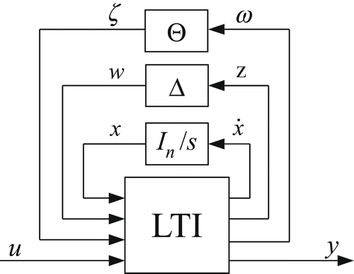
This formalism can be very useful both for robust control analysis [14] and for grey-box parameter identification [12,15]. Tools and algorithms are now being developed which allow us to perform the transformation from Equation (1)(1) [16,17] or (3) [18] to Equation (5)(5) automatically.

Another popular formalism is that of Linear Parameter Varying (LPV) systems, which is the basis for many gain scheduling control design techniques (see the survey papers [19,20]). The system model must be formulated as

The system matrices depend on the time-varying vector of scheduling variables ρ(t), which is assumed to be measurable, and thus known to the controller. The vector ρ may include some of the system states, as well as known functions of the system inputs, in which case the model is known as quasi-LPV. There might be different assumptions about the dependency of the system matrices from ρ, depending on the specific control design techniques. The most common ones are:

• Affine parameter dependence (LPV-A): , and similarly for B, C and D. An extension to polynomial dependence can also be considered.

• Input-affine dependence (LPV-I): as above, but only for matrices B and D, while A and C are constant.

• LFT parameter dependence (LPV–LFT): the dependence on the scheduling parameters is described by an LFT, such as in Equation (5)(5), with .

The reduced-order model should eventually be cast in the above-mentioned formulations, with the minimum possible complexity which is compatible with a good performance of the closed-loop control systems. This can be either checked empirically a posteriori through closed-loop simulation with the full model or formally proven a priori through robust control analysis techniques, in case it is possible to quantify the approximation inherent in the MOR phase in a way which is compatible with the robustness analysis technique.

For all possible kinds of controller, minimum complexity means first and foremost the lowest possible number of state variables, to keep the complexity of the controller design phases and of the implemented control law at a reasonable level. It might also mean that only the non-linearities that are effectively influencing the system behaviour over the expected operating range are considered, to avoid unnecessarily conservative and/or complex designs. For this reason, local approximation techniques, which only try to approximate the system behaviour around specified reference trajectories, are definitely useful.

For most design techniques, where the bulk of the computation is done off-line during the controller synthesis phase, it is not essential that the reduced-order model is also fast to compute, as the design phase is done once and for all, and not in real time. A situation where, for example, the computation of f (x, u) might require the iterative solution of implicit equations might still be acceptable. On the contrary, models for MPC control require us to compute the right-hand-side of the state-space equations many times at each time step by non-linear optimization algorithms that must run in real time; in this case, it is absolutely essential that the speed of computation is as fast as possible.

2.4. Strategies for control-oriented MOR of object-oriented models

The starting point for the generation of a reduced-order, control-oriented model from an object-oriented model is the set of index-1 DAEs (2) obtained from the O–O compiler. This model can be brought into standard state-space form Equation (3)(3) by solving it for the unknowns through a suitable combination of symbolic and numeric techniques, which are routinely implemented in O–O tools to produce the simulation code. Two different strategies can then be followed to obtain a reduced-order model. The first option is to first bring the full DAE model into state-space form, and then apply MOR techniques for ordinary differential equation (ODE) models; the other option is to apply MOR techniques for DAE models to the full DAE model, and then bring the reduced-order DAE in state-space form at the end of the process. Techniques to support both strategies will be reviewed in the next section.

3. MOR techniques for non-linear systems

3.1. Trajectory PieceWise-Linear approximation

The non-linear dynamical system considered in the Trajectory PieceWise-Linear (TPWL) approximation is given in the state-space form [21]:

(6)

where is the state vector, is a non-linear vector-valued function, B is an n × m input matrix, is the system input, C is a p × n output matrix and is the output.

The TPWL technique is based on a quasi-piecewise-linear approximation of the function f, around s linearization points (states) :

(7)

where A_i are the Jacobians of f evaluated at states x_i and 's are state-dependent weights (, for all x). Linear MOR can be then applied to each linearized system:

(8)

through some classical techniques, based on the construction of an orthonormal basis , with , spanning the most significant dynamics. Thus, assuming , where is the reduced state-space vector, one obtains:

(9)

where w_i (z)s are weights dependent on the reduced-order state z (, for all z). These weights are computed based on the distances between the current state and the linearization points (see Ref. [22]), with a rapid transition from one linearization point to another, so that a single linearized model is actually dominant for most of the state space (in this sense (9) is a piecewise-linear model). For example, in Ref. [23] the following weighting scheme is proposed:

(10)

where β is a positive constant, , with z_i being the projection of the linearization state x_i and .

As far as the choice of a suitable projection basis V is concerned, various techniques may be considered. For example, a set of Krylov subspaces could be determined for different linearized model and then merged together, or the projection could be computed according to a Truncated Balanced Realization (TBR) techinque, or a hybrid combination of both approaches ([24–26 26]). In this last case, a singular value decomposition (SVD) on the projection matrix V is performed, and only vectors corresponding to the largest singular values are selected as the columns for a new reduced projection matrix. An alternative technique could also be considered to generate the projection matrix: the Proper Orthogonal Decomposition (POD) [27]. This technique is based on a snapshot of the system solution, obtained, for example, by simulation: and computes a basis V minimizing the overall projection error . The solution is hence given by the SVD on the data collection , where V is made up by the dominant singular vectors.

The choice of the linearization points is also crucial. To limit the computational burden, while spanning the n-dimensional state space of the original model (6), the authors propose to generate a collection of models selected from a single training trajectory, corresponding to some relevant training input, by performing a simulation of the full-order non-linear system. Of course, the reduced-order model is accurate as long as its trajectories are not too far from the training one.

3.2. Piecewise-linear parameterized MOR

In Ref. [21], the authors also proposed a method for estimating a posteriori the approximation error, based on the estimation of the norm of the Hessian of function f, moreover, some results on the stability and passivity of the reduced-order model are derived. If the original non-linear system is L_p -stable and the input signal is bounded, the difference δx between the state of the full-order non-linear model and the state of the piecewise-linear approximated model is bounded, provided that all matrices are symmetric and strictly stable or all matrices are strictly diagonally dominant, with all diagonal elements being negative. Moreover, if 0 is an exponentially stable equilibrium point for system , there exists a stability-preserving weighting procedure.

In Ref. [23], the TPWL technique is extended by considering a non-linear dependence of system (6) from some parameters:

(11)

where is a vector of parameters then, by polynomial fitting or Taylor series approximation, the dependence of the parameters is extracted from the non-linear functions:

For example, a first-order Taylor series expansion on f (x, p) in the neighbourhood of a nominal value of parameters yields

By introducing a new set of parameters, it is finally possible to obtain

(12)

The TPWL technique may now be applied to Equation (12)(12) similar to Equation (7)(7), while considering the parameter dependence of the system, obtaining

Again, standard projection techniques can be applied to each linearized system in (3.2) obtaining

(note that the constant vector k_ij may be treated as a second input vector B ₂ with a constant input ).

The authors suggest in Ref. [23] selecting the linearization points with additional trajectories with respect to the training inputs considered in the standard TPWL, relevant to a set of nominal points in the parameter space. In particular, training should be performed in regions where the system is more sensitive to each parameter (the authors also show how to estimate the sensitivity of trajectories to parameter variations).

They also suggest simulating a linearized model, instead of the full non-linear system, to evaluate the training trajectories: once the current simulated state leaves the neighbourhood of a linearization point, a new linearized model is created at the current state. It must also be pointed out that the additional trajectories relevant to parameter-space training increase the cost of construction the model but not its simulation, since the weighting functions are typically non-zero for few models at any given time.

3.3. MOR based on PieceWise Polynomial representation

Very recently, a new method has been proposed to overcome a limitation of TPWL methods [4], namely, the fact that these methods provide accurate results for large-signal transient analyses, in that they capture strong non-linearities well in a wide range, but may fail for small-signal distortion analysis. The reason is that when considering a trajectory close to a linearization point, the TPWL model reduces to an LTI system and no distortion can be captured. Essentially, the new method: PieceWise Polynomial (PWP) is based on a higher-order (tensor) polynomial approximation rather than a simple linear one as in TPWL, capturing small-signal distortion well around the expansion point.

Again, s points x_i are considered in the state space () but, instead of a first-order expansion as in the TPWL, a higher-order expansion is performed, for the sake of simplicity a quadratic expansion will be considered:

where matrix A _2,i collect the second-order derivatives of f(x) and the symbol ⊗ represents the Kronecker tensor product.

A projection basis V_i can be constructed for each expansion point by applying a weakly non-linear MOR technique, and a uniform projection base is then generated through SVD on the collection of all basis . The final reduced-order PWP model is again obtained by a weighted combination of models:

where , , and .

Some comments are now in order about the weakly non-linear MOR techniques. Consider a polynomial expansion of f (x) around a DC operating point:

(13)

where A_i is the i-th order derivative. According to the Volterra theory [28], the solution of Equation (13)(13) is the sum of different responses:

where each response x_i  (t) can be recursively computed by solving the same LTI with different inputs. For example, the first- through the third-order responses are the solutions of the following linear systems:

(14)

(15)

(16)

The problem has been therefore recasted as a reduction of a series of LTI.

The simplest way to deal with the reduction of this form is to separately reduce each LTI [29], for example, by Krylov subspace computation, by plugging the response of each system as an input to the following LTI in the series. For example, assume that the first-order LTI (14) is reduced by the projection base V ₁, then the response can be approximated as and plugged into the second-order LTI (15) having as input

for which another projection base V ₂ can be determined and so on. However, in this way the dimension of the projection base rapidly increases, resulting in inefficiently large reduce models. A more compact projection base V could be computed through SVD on the collection of separated basis [30], that is, but the improvement is in general scarcely appreciable. The most efficient way to approach the problem is the Non-linear Model Order Reduction Method (NORM)–Momentwise Projection [31], which obtains a very compact reduced model without loss of accuracy by removing some redundancies among the Krylov subspaces of each LTI system in the series. Anyway, in Ref. [4] an alternative to NORM is presented, namely, the MPI method, which exploits the intrinsic correlation among the inputs to the LTI in series.

The PWP method is also endowed with an heuristic algorithm to choose expansion points to cover a wide range of the state space with limited expansion regions. Essentially, a new state is added to the expansion point set when the relative error between the current evaluation of f (x) and its linearization exceeds a predefined error tolerance along the training trajectory. Another improvement in efficiency is obtained by merging regions from different trajectories, to maximize the state-space coverage. Thus, new points on new trajectories are added to the base set of expansion points only if the distance between the new points and the points already in the base set is greater that some predefined tolerances.

Finally, some limitations of the choice (10) for the weighting functions were pointed out in Ref. [4], namely, the fact that sometimes the error is large when the current state is on the border of the space covered by the expansion points. The authors then propose the following expression for the weighting function:

where , , D _min is the minimum distance among the base set points z_i , whereas parameter p is used to make the transition smoother or shaper when switching from one region to another. The whole weight function is finally normalized to satisfy .

3.4. Simulation-free NORM

A rather different approach to NORM, thus not based on linearization nor on simulation, has been proposed in Ref. [32]. The key idea of the method is to separate the original non-linear model into a linear and a non-linear part, and to consider the non-linearities of the resulting system as additional inputs to the linear part.

The method considers a general non-linear time-invariant system:

which can be rewritten as

(17)

where the vector g (x, u) collects the non-linear parts of the element of f (x, u), in such a way that every non-linear term appears only once and is free from any possible constant factor. In turn, by defining a new input matrix and a new input model (17) can be rewritten in the form

(18)

If u* is actually considered as an exogenous input, which it is not because it depends on the state x, the order of system (18) can be reduced through any MOR technique for LTI systems:

(19)

Finally, if an approximation of the state vector is considered in g (x, u), just derived from Equation (19)(19), thus or, more generally, , the overall reduced-order model can be defined by a feedback connection of Equation (19)(19) and :

or

Authors in Ref. [32] suggest the adoption of Eitelberg's order reduction method [33], which they extend to find suitable matrices W ₁ and W ₂. As in the original method, the solution is found by minimizing the error between the step responses of the full system and the reduced-order system, after defining a set of dominant state variables and imposing a null steady-state error for the reduced linear model. Actually, a sub-optimal solution is computed, minimizing the time-dependent term of the error to find W ₁ and vanishing the time-independent term by a suitable choice of W ₂.

3.5. Analytical MOR based on symbolic analysis

An even more different approach is described in Refs. [6,34,35], where the dominant system behaviour is extracted by automated derivation of approximated symbolic formulas, by means of mixed symbolic (computer-algebra) and numerical strategies. One major advantage of this approach is that it can be applied to a very general non-linear DAE system in form (2).

A key aspect of the method is that a symbolic formulation of the DAE system is considered, in other words, a complete class of models with arbitrary parameter values. Another advantage is that the accuracy of the reduced-order model can be predefined and automatically checked, and the result of the simplification maintains a physical interpretation. The method is original from the field of the analog electronic circuits design, but it can be extended to general equation-based, acausal modelling environments.

The equation-based approximation process can be sketched as follows:

1. A general symbolic DAE system and a list of numerical reference values are first generated.

2. Based on the said reference values, the system of equations is evaluated and numerically solved for some variables of interest.

3. The results are compared with a simulation, to ensure that the equations are correct and the symbolic model reduction can start.

4. Because the model reduction consists in a sequence of symbolical simplification steps, it is fundamental to predict the influence on the error with respect to an objective function a simplification step causes. This prediction is performed by a ranking algorithm that orders simplification steps according to the error generated [36]. One way is to iteratively applying each simplification step to the original system and carrying out one single Newton step starting from the reference solution, the corresponding deviations set up the ranking order.

5. The next step applies the simplification (or a cluster of simplifications having the same order of magnitude in the ranking), the accumulated error is calculated and compared with the given error bound. If the error bound is exceeded, the algorithm terminates returning the approximated system, otherwise the next simplification steps from the ranking list are carried out.

Several simplification strategies may be applied: algebraic simplification (variable elimination and decoupling of blocks), branch simplification (deletion of branches of piecewise-defined solution), switch simplification (fixing of values of switch variables), term substitution (replacement of variables with mean values obtained in reference simulations) and term deletion (removal of terms in equations).

One important point to remark upon is the fact that simplifications may increase the index of the DAE system (2), thus preventing the numerical solution with standard solvers [37]. As a consequence, an index observer must be integrated in the simplification algorithm to monitor and avoid index increase.

4. Extensions and future research directions

The MOR methods described in this survey are generally applied to the design of integrated micro-electro-mechanical systems (MEMS) and electronic circuits. Within this application domain, the objective is to obtain reduced models to support the integrated system design through virtual prototyping techniques. This kind of models can contain strongly non-linear components, but the external inputs to the system–typically current and voltage generators–appear as linear terms. This consideration results in a simplification of the mathematical formulation of the dynamic model, that can be represented as an ODE system which is linear in the inputs (6). When taking into account generic models of multi-domain dynamic systems, this formulation might not be general enough. It would then be interesting to extend the TPWL techniques to the more generic non-linear systems (3), which could be obtained after index reduction and reformulation as ODEs.

Another issue with existing TPWL techniques is that they usually employ a Krylov-based approach for the reduction of the linearized models, which requires those models to have no poles in the origin. This is not a problem with typical MEMS and electronic circuits, which always have finite DC gains, but might be an issue with generic object-oriented models that contain pure integrators. In this case, different methods for the local approximation of the linearized systems should be investigated.

The methods described in Section 3.5, although initially developed for electronic circuits, have already found some applications in other domains, as shown in Ref. [6]. It would be interesting to test those methods with a wider range of multi-physics model, obtained from object-oriented models written in Modelica. It might as well be interesting to embed index reduction techniques in these methods, to allow an even more aggressive order reduction.

It will also be necessary to investigate how well different MOR techniques can match the specific formalisms required by the different control design techniques, both from a theoretical point of view and through testing on specific applications.

Another promising research direction could be to explicitly consider the information that is available on the topological representation of the dynamic system before obtaining the abstract mathematical representation (as DAE or ODE). Several works are present in literature considering mechanical applications. In particular, an ‘Energy-Based Model Reduction’ is proposed in Refs. [38,39], using the bond graph approach. Even if this could lead to some advantages, the limitation of the proposed methods is quite restrictive, because it is only possible to use bond graph connectors when creating a model. An improvement in the direction of supporting more general object-oriented models could be to extend these techniques considering also more general connectors.

Obtaining effective results in this field would require the integration of different tools (Modelica compilers, symbolic manipulation tool, numerical tools), possibly developed within different communities. More generally, a closer interaction between research groups working in different areas, like electronic circuit design, modelling and simulation and control theory, would be helpful to obtain better results for everyone.

5. Conclusions

Object-oriented modelling methodologies, and in particular the Modelica language, are emerging as a tool for system design, but their use is currently mostly limited to simulation activities. On the other hand, the control system (and thus its design) is a key part of all modern integrated systems.

The models which are required for the control system synthesis have rather stringent requirements in terms of simplicity and of specific mathematical structures, which are discussed in this article. In particular, MOR is essential to obtain models which are simple enough to be directly used for that purpose. This activity is nowadays performed manually, and there is thus a clear need of methods and tools to perform this task automatically, starting from object-oriented descriptions of the plant.

Several MOR techniques, which have been recently introduced by the electronic circuit design community, have been reviewed in this article. Much work remains to be done to adapt and possibly extend them to work satisfactorily when dealing with generic object-oriented models; some possible research lines have then been proposed in this direction.

References

- Casella , F. , Donida , F. and Lovera , M. 2008 . Beyond simulation: computer aided control system design using equation-based object oriented modelling for the next necade . 2nd International Workshop on Equation-Based Object-Oriented Languages and Tools . July 8 2008 , Paphos, Cyprus. pp. 35 – 45 . Linköping University Electronic Press .
- Feng , L. 2005 . Review of model order reduction methods for numerical simulation of nonlinear circuits . Appl. Math. Comput , 167 : 576 – 591 .
- Feng , L. 2005 . Parameter independent model order reduction . Math. Comput. Simulat , 68 : 221 – 234 .
- Dong , N. and Roychowdhury , J. 2008 . General-purpose nonlinear model-order reduction using piecewise-polynomial representations . IEEE Trans. Computer-Aided Des. Int. Circuits Syst. , 27 : 249 – 264 .
- Schwarz , P. , Bastian , J. , Clauss , C. , Haase , J. , öhler , A. K , Otte , G. and Schneider , P. 2007 . A tool-box approach to computer-aided generation of reduced-order models . EUROSIM 2007 . September 2007 , Ljubljana, Slovenia. pp. 9 – 13 . EUROSIM .
- Sommer , R. , Halfmann , T. and Broz , J. 2008 . Automated behavioral modeling and analytical model-order reduction by application of symbolic circuit analysis for multi-physical systems . Simul. Model. Pract. Theory , 16 : 1024 – 1039 .
- Mattsson , S.E. , Elmqvist , H. and Otter , M. 1998 . Physical system modeling with Modelica . Control Eng. Pract , 6 : 501 – 510 .
- Fritzson , P. 2004 . Principles of Object-Oriented Modeling and Simulation with Modelica 2.1 , Piscataway, NJ : 1 Wiley-IEEE Press .
- The Modelica Association, Modelica Home Page. Available at http://www.modelica.org (http://www.modelica.org)
- Mattsson , S.E. and öderlind , G. S . 1993 . Index reduction in differential-algebraic equations using dummy derivatives . SIAM J. Sci. Comput , 14 : 677 – 692 .
- Ljung , L. 2008 . Perspectives on system identification . 17th IFAC World Congress . July 2008 , Seul, South Korea. pp. 6 – 11 . Curran Associates, Inc .
- Casella , F. and Lovera , M. 2008 . LPV/LFT modelling and identification: overview, synergies and a case study . 2nd IEEE Multi-conference on Systems and Control . September 2008 , San Antonio, Texas, USA. pp. 3 – 5 . IEEE .
- Qin , S.J. and Badgwell , T.A. 2003 . A survey of industrial model predictive control technology . Control Eng. Pract. , 11 : 733 – 764 .
- Zhou , K. , Doyle , J.C. and Glover , K. 1996 . Robust and Optimal Control , Englewood Cliffs, NJ : Prentice-Hall .
- Hsu , K. , Vincent , T. , Wolodkin , G. , Rangan , S. and Poolla , K. 2008 . An LFT approach to parameter estimation . Automatica , 44 : 3087 – 3092 .
- Casella , F. , Donida , F. and Lovera , M. Automatic generation of LFTs from object-oriented non-linear models with uncertain parameters . MATHMOD 2009, ARGESIM Report no. 35 . 2009 . Vienna, Austria, 11–13 February
- Casella , F. , Donida , F. and Lovera , M. 2008 . Automatic generation of LFTs from object-oriented Modelica models . 2nd IEEE Multi-Conference on Systems and Control . September 2008 , San Antonio, Texas, USA. pp. 3 – 5 . IEEE .
- Magni , J.F. 2006 . User manual of the Linear Fractional Representation Toolbox, version 2.0 , ONERA : TR 5/10403.01F DCSD .
- Leith , D.J. and Leithead , W.E. 2000 . Survey of gain-scheduling analysis and design . Int. J. Control , 73 : 1001 – 1025 .
- Rugh , W. and Shamma , J. 2000 . Research on gain scheduling . Automatica , 36 : 1401 – 1425 .
- Rewiénski , M. and White , J. 2006 . Model order reduction for nonlinear dynamical systems based on trajectory piecewise-linear approximations . Linear Algebra Appl. , 415 : 426 – 454 .
- Rewiénski , M. and White , J. 2002 . A trajectory piecewise-linear approach to model order reduction and fast simulation of nonlinear circuits and micromachined devices . IEEE Trans. Computer-Aided Des. Int. Circuits Syst. , 22 : 155 – 170 .
- Bond , B. and Daniel , L. 2007 . A piecewise-linear moment-matching approach to parameterized model-order reduction for highly nonlinear systems . IEEE Trans. Computer-Aided Design of Integrated Circuits Syst. , 26 : 2116 – 2129 .
- Muscato , G. 2000 . Parametric generalized singular perturbation approximation for model order reduction . IEEE Trans. Automatic Control , 45 : 339 – 343 .
- Shi , G. and Shi , C.J.R. 2005 . Model-order reduction by dominant subspace projection: error bound, subspace computation and circuit applications . IEEE Trans. Circuits Syst. , 52 : 975 – 993 .
- Wong , N. , Balakrishnan , V. , Koh , C. and Ng , T. 2006 . Two algorithms for fast and accurate passivity-preserving model order reduction . IEEE Trans. Computer-Aided Des. Int. Circuits Syst. , 25 : 2062 – 2075 .
- Rathinam , M. and Petzold , L. 2003 . A new look at proper orthogonal decomposition . SIAM J. Num. Anal. , 41 : 1893 – 1925 .
- Rugh , W. 1981 . Nonlinear System Theory-The Volterra Wiener Approach , Baltimore, MD : Johns Hopkins University Press .
- Roychowdhury , J. Reduced-order modelling of linear time-varying systems . IEEE/ACM international conference on Computer-aided design ICCAD '98 . New York, NY. pp. 92 – 95 . San Jose, CA : ACM .
- Phillips , J. 2000 . Projection frameworks for model reduction of weakly nonlinear systems . IEEE Design Automation Conference . June 2000 , Los Angeles, CA. pp. 5 – 9 . 184 – 189 . IEEE .
- Li , P. and Pileggi , L.T. 2003 . NORM: compact model order reduction of weakly nonlinear systems . Design Automation Conference . June 2003 , Anaheim, CA. pp. 2 – 6 . 472 – 477 . IEEE .
- Salimbahrami , B. and Lohmann , B. 2004 . A simulation-free nonlinear model order-reduction approach and comparison study . Math. Computer Model. Dyn. Syst. , 10 : 317 – 329 .
- Eitelberg , E. 1981 . Model reduction by minimizing the weighted equation error . Int. J. Control , 34 : 1113 – 1123 .
- Wichmann , R. , Popp , R. , Hartong , W. and Hedrich , L. 1999 . On the simplification of nonlinear DAE systems in analog circuit design . 2nd Workshop on Computer Algebra in Scientific Computing, CASC ‘99 . June 1999 , Munich, Germany. 31 May–4 . Springer Verlag .
- Mikelsons , L. , Ji , H. , Brandt , T. and Lenord , O. 2009 . Symbolic model reduction applied to realtime simulation of a construction Machine . 7th International Modelica Conference . September 2009 , Como, Italy. pp. 20 – 22 . Modelica Association .
- Halfmann , T. and Wichmann , T. 2006 . “ Symbolic methods in industrial analog circuit design ” . In Scientific Computing in Electrical Engineering , Edited by: Anile , A.M. , Ali , G. and Mascali , G. Springer Heidelberg .
- Ascher , U.M. and Petzold , L.R. 1998 . Computer Methods for Ordinary Diferential Equations and Differential-Algebraic Equations , Philadelphia, PA : SIAM .
- Loucas , L.S. and Stein , J.L. 1999 . Energy-based model reduction of linear systems . 4th International Conference on Bond Graph Modeling and Simulation ICBGM'99 . January 1999 , Francisco, CA. pp. 17 – 20 . SCS Publishing, San .
- Loucas , L.S. and Yildir , U.B. 2006 . Modelling and reduction techniques for studies of integrated hybrid vehicle systems . Math. Computer Model. Dyn. Syst. , 12 : 203 – 218 .