Reconstructing the knee joint mechanism from kinematic data

Abstract

The interpretation of joint kinematics data in terms of displacements is a product of the type of movement, the measurement technique and the underlying model of the joint implemented in optimization procedures. Kinematic constraints reducing the number of degrees of freedom (DOFs) are expected to compensate for measurement errors and noise, thus, increasing the reproducibility of joint angles. One approach already successfully applied by several groups approximates the healthy human knee joint as a compound hinge joint with minimal varus/valgus rotation. Most of these optimizations involve an orthogonality constraint. This contribution compares the effect of a model with and without orthogonality constraint on the obtained joint rotation angles. For this purpose, knee joint motion is simulated to generate kinematic data without noise and with normally distributed noise of varying size. For small noise the unconstrained model provides more accurate results, whereas for larger noise this is the case for the constrained model. This can be attributed to the shape of the objective function of the unconstrained model near its minimum.

Keywords:

• tibiofemoral joint
• kinematics
• optimization
• compound hinge joint
• model comparison
• sensitivity analysis

1. Introduction

The relevance of understanding knee joint kinematics reveals itself in a number of clinical topics. For instance, prostheses have to be designed so that the flexibility and stability characteristics of the human knee joint are reproduced as close as possible to limit loosening and accelerated wear. During surgical intervention of lower-limb alignment, it is also very important to consider joint kinematics.

The interpretation of joint kinematics strongly depends on the measurement process. When using opto-electronic, magnetic or medical imaging techniques markers may be placed invasively or on the skin, the latter involving soft tissue artefacts [1,2]. Further sources for differing interpretations evolve from the measurement protocol including the marker set and kind of the investigated movement.

An important source for discrepancies between different studies is the fact that the calculated rotation angles strongly depend on the way how the axes locations are defined [3]. For a given definition of the joint rotation axes, the acquisition of anatomical landmarks by palpation is an additional source of error and high intersession variabilities. Thus, functional methods independent of anatomical landmarks are to be preferred, that is, the kinematic marker data of two adjacent body segments are matched with a kinematical model to find the joint rotation axes [4]. In some cases, for example, if the range of motion in the concerned joints is too small, functional methods are not applicable. In many clinical applications, the acquisition of full 6 degree of freedom (DOF) knee joint motion data is not required because of the reliability of the measurement techniques [5]. A simplified model of the knee joint may lead to a higher reproducibility. It is expected that an appropriate model compensates for the measurement errors and reduces the effects of noise. However, using a model means that the solution is sought in the subspace defined by the model constraints and further realities could be concealed.

The aim of this contribution is to quantify the influence of previously applied kinematic models described in Section 2.2 on the interpretation of measurement data. Section 2.1 describes the present conclusions about the location of the axes of a healthy human knee joint due to empirical studies. These empirical investigations formed the basis for the simulation of the knee joint motion and the generation of data from a kinematic measurement. Models approximate the real geometry of the joint. In this study a model was constructed matching the geometry of the knee joint closer than previously applied ones. The calculated joint axes and angles due to the above-mentioned new model and a previously applied model were compared for simulated kinematic data without noise and with normally distributed noise of varying size. It is expected that the noise level determines whether a model closer to the geometry of the simulation involving more DOF or a more constrained model has to be preferred.

2. Current models describing human knee joint kinematics

2.1. Models using anatomical landmarks

The human knee is composed of two joints, the patellofemoral and the tibiofemoral joint (TFJ). Here we focus on the TFJ which was intensively studied in the past, involving a paradigmatic shift in the understanding of human knee joint kinematics. Based on observations in the sagittal plane, that is, in two dimensions, it was concluded that the knee has no fixed flexion/extension (FE) axis. However, the plane of the FE movement and the sagittal observation plane are tilted by about 5–10° [6,7]. Thus, even a fixed axis seems to move as a result of the tilt [8,9].

Currently, it is widely accepted that within achievable accuracy the FE axis is fixed in the posterior femoral condyles [9]. Observations from active and passive movement are consistent. The assumption of a fixed FE axis is supported by the fact that isometric points on the distal femur – the femoral attachments of the collateral and the cruciate ligaments – can be found [10]. However, there exist several different definitions of the FE axis on the basis of anatomical landmarks. Several authors compare the clinical and the surgical transepiconylar axis, the functional FE axis and the cylindrical (geometric centre) axis [9,11,12].

According to [9], TFJ motion can be represented as a pair of independent rotations about two axes. The FE axis is fixed with respect to the femur and the tibial rotation (TR) axis is fixed in the tibia. Femoral rollback is then the manifestation of tibial (longitudinal) rotation during knee flexion. It was found in [13] that the TR axis was anterior to the FE axis (i.e. there is no intersection) and not perpendicular to it. The compound hinge theory was tested by estimating the error made as a consequence of the assumption of the two-fixed-axes model [14]. The compound hinge model is supported by observing minor residual displacements only [7,15].

The choice of the axes system is substantial. For a mechanical linkage it was demonstrated that an improper selection of the FE and TR axes can result in a virtual screw home motion [16]. Therefore, angles from different studies become comparable first when they are recalculated for the same system of axes.

Additionally, tibial rotation can be influenced by external forces and there is no strict correspondence between extension and tibial rotation [8,17]. The location of the observed TR axis is task-dependent. Therefore, it is necessary to specify the movement task in combination with the recorded joint kinematics.

Further in vitro research identifies two FE axes, one acting in the regime of 150° to 15° of knee flexion and one in the regime until full extension [8,10].

Summarizing this section, it can be stated that the healthy human tibio-femoral joint can be approximated by a model exhibiting two fixed axes [8–11,13,15,18]. For the following investigations, we assume that the TR axis is fixed and the plane of the FE movement is tilted with respect to the sagittal plane [13].

2.2. Models using kinematic observations and optimization

An important aim in the biomechanical analysis is the reproducible and user-independent description of joint kinematics. With this objective, the positions and orientations of the axes within femur and tibia can be considered as model parameters. By introducing additional constraints like orthogonality and/or intersection of the axes, the number of parameters can be reduced. The model parameters can be optimized to ‘minimize the difference’ of the measured kinematic from the kinematic predicted by the model. It is hypothesized that the optimization procedure will lead to a unique solution with a well-defined FE and TR axes. As a result of this procedure, the positions and orientations of the FE and TR axes do not depend on anatomical landmarks but are a result of joint kinematics. Surgical interventions, such as ligament repair or total knee arthroplasty, could profit from interoperative kinematic alignment based on an improved procedure of the joint axes determination.

For the purpose of error compensation, existing optimization procedures take advantage of the fact that under load bearing the finite helical axis (FHA) remains fairly stable between 40° and 80° of flexion [19]. The average FHA in this interval is then defined as the FE axis [20,21]. The interval 0° to 40° of knee flexion is dominated by flexion and tibial rotation. According to [20], the adduction/abduction and internal/external rotation axis can be selected to form an orthogonal triplet with the FE axis under the constraint of minimizing the adduction/abduction movement in that interval. Another optimization procedure aims at increasing the reproducibility of hip axial rotation angles [22,23]. In contrast to the former model, not the average FHA, but the line connecting the medial and the lateral femoral epicondyles is defined as the FE axis. The optimized lower-limb gait analysis (OLGA) technique takes into account not only the kinematic constraints imposed by the knee joint but also those due to the hip and the ankle joint [21]. The functional method proposed in [24] uses the floating axis description by defining the first axis (FE axis) perpendicular to the positions of the tibia during the passive range of movement and the second body fixed axis (TR axis) as the component of the helical axis at 90° of flexion perpendicular to the first axis.

The models described above assume that the FE and the TR axes are coplanar and orthogonal. This is in contrast to the findings of [13] where an oblique angle between non-intersecting axes is considered, see Section 2.1. Although in [14] the authors do not restrict the axes to be coplanar and orthogonal, they fix the direction of the FE and the TR axes due to anatomical landmarks. Therefore, only the location of the TR axis is optimized. In [25], however, intersection of the FE and the TR axes is taken into account and treated as the ‘centre of the joint’. This represents a 2 DOF spherical joint [5].

3. Methods

3.1. Kinematic model

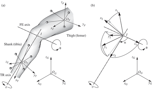
The model introduced here to describe the TFJ consists of intersecting FE and TR axes with an oblique angle between them (Figure 1(a)). Then the intersection I can be obtained as the joint centre by means of coordinate transformation methods or sphere-fitting methods. It is further assumed that the direction of the FE axis can be directly calculated in an interval dominated by pure FE movement and negligible tibial rotation. The introduction of an orthogonality constraint between FE and TR axes corresponds to the models described in Section 2.2 (excluding [14,15]).

Figure 1. (a) Marker clusters generally moving with respect to global coordinate system O _G (x _G , y _G, z _G ) are used to define local coordinate systems (LCS) fixed in the femur O _F (x _F , y _F, z _F ) and in the tibia O _T (x _T , y _T, z _T ), respectively. In the present model the FE and the TR axes intersect at point I but need not to be orthogonal. Angle describes the FE-movement whereas describes the tibial rotation. (b) Two additional LCS are defined. The first is fixed in the femur (x ₁, y ₁, z ₁), and the second is fixed in the tibia (x ₂, y ₂, z ₂). The origins of the two LCS coincide with the point I. The axis lies in the FE axis whereas coincides with the TR axis. The angle represents the angle between FE and TR axes.

Observing knee joint kinematics is normally done by capturing the relative motion of femur and tibia using either markerless medical imaging techniques (e.g. fast-PC-MRI, X-ray flouroscopy and so on) or marker-based methods. In the latter case, the motion of the bones is recorded either directly using cortical bone pins or indirectly using skin-mounted markers leading to additional measurement errors (soft tissue artefacts). All of the above techniques allow for the computation of a time-dependent local coordinate frame for the thigh (femur) and shank (tibia). Such a time series of two coordinate frames, in general, is the starting point for the calculation of joint axes or centres by means of coordinate transformation and sphere- or centre-fitting methods [26–28]. The symmetrical axis/centre of rotation estimation (SCoRE) calculates the transformation matrix and the vector , which at time describes the orientation and translation of the segment's coordinate system with respect to a predefined reference orientation and position [27]. Herein j = 1,2 denotes the number of the segment. Although both segments may move arbitrarily with respect to a global frame of reference (global coordinate system, GCS), it is assumed that a centre of rotation (CoR) or even an axis of rotation (AoR) for the relative movement can be found. Let be the CoR fixed in the LCS of segment j, then the position vector of the CoR in the GCS is given by

(1)

corresponding to a generalization of Equation (17) in [27]. The estimation of the CoR or AoR is based on the following linear least squares problem,

(2)

compare Equation (20) in [27] or Equation (2)(2) in [28]. As a consequence of the measurement noise, the global CoR calculated from and do not necessarily coincide, thus, it is suggested to define in the GCS as the mean between these two positions [27].

Formally, Equations (1)(1) and (2) are identical for CoR or AoR. It depends on the type of movement and on the joint in question whether it is possible to determine a single axis or a CoR. In the case of a planar rotation, the matrix of rotation matrices on the left-hand side of Equation (2)(2) has rank five (for exact data). Thus, the result of the minimization has to be an AoR, not a CoR. Measurement noise virtually increases the rank of matrix. A criterion for a planar rotation is that the value of the sixth singular value is small compared with the five others.

For a number of applications, a fixed CoR or AoR may be a poor approximation to describe joint kinematics. Then only an instantaneous axis will be defined. For a joint with pure rotations this axis follows from Equation (2)(2) solved in a given time slot t. In the case of a general displacement including both translations and rotations the FHA can be calculated [29]. Provided that this is not a pure translation, the two configurations at times and are related to each other by a rotation about and a translation along a uniquely defined axis, the FHA.

The approach introduced in this article approximates the healthy knee joint by a compound hinge joint. The optimization procedures assume that the FE axis can be computed in an interval of pure flexion by means of Equation (2)(2). If the two axes intersect, the centre of the joint I is defined as the solution of Equation (2)(2) within the full range of movement. Because the direction u _FE and the location of the FE axis and the intersection I can be calculated, it is convenient to discuss and solve the problem in a coordinate system where I coincides with the origin and u _FE lies in the axis (Figure 1(b)).

In coordinates of the local femur coordinate system (LCS 1), the orthogonal tibial basis frame at time reads

(3)

The index 1 in denotes that the tibial basis frame is written in the coordinates of the femur system LCS 1. Not only the tibial basis frame obeys Equation (3)(3), any point fixed with respect to tibia transforms in the same way. The function describes the time-dependent relative orientation of the two bodies and will be parameterized as follows,

(4)

where and act as a rotation by an angle about the x and the z axes, respectively. A rotation about the FE axis simply coincides with a rotation about the z axis. The direction of the TR axis is obtained by rotating the vector about the two angles and , see Figure 1(b). The unknown parameters are then the time-dependent flexion angle , the time-dependent tibial (=internal/external) rotation angle and the two angles and describing the relative location of the TR axis with respect to the FE axis.

To reduce the number of unknown parameters, an ansatz for and has to be implemented. The introduction of such a functional approach has to reflect the reality as close as possible because an unsuitable approach may lead to different kinematic interpretations. Obviously, the shape of the curves for and depends on the type of movement. The authors therefore suggest selecting an initial shape function as a first guess based on the current data. After the parameters have been optimized, new shape functions can be generated to iterate the process of the optimization. The iterative procedure aims at the reduction of the manipulative effect of an ansatz function arbitrarily fixed by the observer. Finally, the functions are expected to approach the real shape of and .

In Figure 2 different shapes of the functions and are compared. Figure 2(a) shows different types of passive knee flexion, with and without external load whereas Figure 2(b) demonstrates gait data. As it can be seen in Figure 2, external load stabilizes in the range of [31]. As an input for the optimization procedure a squat movement was also successfully used, see, for example, [20]. In kinematic data from gait analysis, the range of flexion in the stance phase (support phase of body weight) is fairly small.

Figure 2. (a) Passive knee flexion with and without external load. Solid line [30]: constraint based model; short dashed line [30]: reference model; dash-dotted line [31]: external torque of 3 Nm; dotted line [31]: internal torque of 3 Nm; long dashed line [32]; (b) FE angle and TR angle during a gait cycle [33]. Note that (b) shows and whereas (a) plots . In addition, the range of is about 90° in (a) and 35° in (b).

In our optimization model, the function was approximated as a function linear in time. As sample functions for , the internal/external rotation curves of [31,32] were approximated by polynomial fits of degree 4. This yields the initial form of the two functions

(5)

(6)

The are the polynomial factors of the shape function . The two angles and representing the orientation of TR with respect to FE and the scaling factors and of the time-dependent rotation angles and are determined in the optimization procedure. Starting from Equation (3)(3), the following objective function has to be minimized,

(7)\

to give the best fit of the model to the given kinematic dataset. The index F denotes the Frobenius matrix norm.

For the numerical solution of the resulting minimization problem, we use the function lsqnonlin from the Matlab ¹ optimization package. Here, the algorithmic variant based on the Levenberg–Marquardt method has turned out to be most robust and effective. This method is based on an adaptive regularization strategy enforcing monotonous decay of the objective function in each iteration step [34].

The optimized parameter set is then inserted in the time series to calculate an error measure, namely, the residual rotation for each step.

3.2. On the uniqueness of the solution

Obviously, the solution in terms of the four parameters is not uniquely defined for only one step from time frame to time frame . Three parameters sufficiently describe this rotation, the rotation axis direction (two angles) and the rotation angle (one angle). By considering at least a second movement step, from time frame to time frame , the solution appears to be unique provided that the movement is not a planar rotation.

To study the behaviour of the minimization problem and the performance of the minimization algorithm in more detail, we first consider a test problem based on data completely consistent with our model, sampled at 10 observation times. For we choose the quartic polynomial fit according to the model from [32]. We choose , , and , and prescribe data exactly fitting our model equations. This means that the prescribed values for and solve the minimization problem, and the residual of the objective function from Equation (7)(7)\ vanishes at the solution. As initial guess for the minimization procedure, however, we choose significantly perturbed values for , with perturbations of the size of up to and more. Matlab/ lsqnonlin returns the true solution up to rounding error, and in all cases tested the convergence behaviour was observed to be regular and monotone.

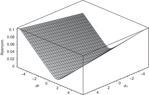
Other algorithmic variants like the classical ‘Gauss-Newton method’, which is usually more sensitive to the geometry of the objective function, show a significantly more irregular convergence behaviour. This may be attributed to the slightly degenerated convexity behaviour of the minimization problem: If we fix and but let and vary about the true solution, the residual, that is, evaluation of objective function features a pronounced ‘valley’ along a curve in the -plane passing through the solution. The minimum is indeed unique, but the values of the residual along this curve are significantly smaller than in the region nearby. This situation is visualized in Figure 3: Here, and are given in degrees, and an appropriately scaled square root of the residual is plotted for the purpose of improved recognizability.

Figure 3. Rescaled values of the residual near the true solution (problem with exact data).

4. Results of the optimization

The optimization parameters in the objective function specified in Equation (7)(7)\ are and . To account for the oblique angle between the two fixed hinge axes (Model 1), the full set of parameters is included into the optimization process. In the model with orthogonality constraint (Model 2), the angle between the FE and TR axes is fixed at and only the remaining three parameters are optimized. Residual rotation is introduced as a measure of the error induced by the above orthogonality constraint. For the time step , the residual rotation is defined as a rotation necessary for the congruency between the tibia frame due to the original data and the tibia frame due to the optimized parameters (Model 1) or (Model 2). This yields the matrix of residual rotation whose complex eigenvalues are related to the residual rotation angles,

(8)

4.1. Model comparison

For the numerical simulation, and are implemented according to Equations (5)(5) and (6) where is fitted to data given in [19] and [32] with a polynomial of degree 4, and fixed at .

In the noise-free case, models one and two are compared for varying in the interval with . When using Model 1, true input parameters of the simulation are recovered and, consequently, no residual rotations arise. For Model 2, the optimized parameters deviate from the true values, unless the input parameter . These deviations are shown in Figure 4 whereas the mean residual rotations are depicted in Figure 5. For the mean residual rotation does not exceed 3° in both of the model functions for .

Figure 4. Differences between the optimized parameters and the true simulation input values for model two with the orthogonality constraint and function fitted to data from [19] (a) and [32] (b).

Figure 5. Residual rotation angles for model two with the orthogonality constraint and fitted to data from [19] (a) and [32] (b).

The influence of the noisy data is analysed for . The data for the investigation are provided as before and altered by adding a normally distributed error (using routine randn from Matlab) to all of the four parameters. Test runs are performed for and . For the same set of values for and , the data simulation and parameter optimization are repeated 20 times. Figure 6 shows the square root of the mean squared difference of optimized and true parameters. For both model functions , the application of Model 1 results in a large deviation in the calculated value of . This can be attributed to the behaviour of the objective function near its minimum, see Section 3.2. The minimum in is not sharply pronounced. The residual rotation angles for models one and two and for both functions are comparably small, see Figure 7.

Figure 6. Noisy data: square root of the mean squared difference for the model parameters in the model without (left) and with (right) orthogonality constraint. The standard deviation of the input parameters is (solid lines) and (dashed lines); : circle; : triangle; : cross; : X. Function is fitted to data from [19] (a) and [32] (b).

Figure 7. Mean residual rotation angles for the model with and without orthogonality constraint. The standard deviation of the input parameters was (solid lines) and (dashed lines). Function is fitted to data from [19] (a) and [32] (b).

5. Discussion and outlook

In this article, the compound hinge joint with intersecting axes was tested for a model with and without orthogonality constraint. The experiments indicate that for the case of a joint with an oblique angle between the FE and TR axes, the unconstrained model matches the data closer than the constrained model. It turns out that for the unconstrained model and the exact data, the error of the numerical approximation for the model parameters stays in the range of the round-off errors. However, in contrast to naive expectations, it is also fairly small for the constrained model. Taking measurement noise into account considerably reduces the differences in both models in context of the achieved accuracy of the model parameters. This can be explained by the fact that the minimum of the objective function is not sharply pronounced in , as it is shown for exact data in Section 3.2. Because of the sharp ‘valley’ along a curve in the -plane, the minimum cannot be found easily. For noisy data the objective function is deformed and, therefore, finding its minimum becomes more difficult. A noise level realistic for skin marker-based motion analysis thus justifies preferring the computationally less-expensive constrained model to the unconstrained model. But it seems to be promising that a modification of the unconstrained model may replace the constrained one.

The behaviour of the objective function described above is based on a small set of numerical experiments. However, it seems to be typical and can also be observed for other data configurations. Because the Levenberg–Marquardt method performs successfully, this seems to indicate a potential direction of refinement. For our model, admissible values for and appear to be correlated. This suggests that restricting the range of admissible values by modelling this correlation in an appropriate way – alternatively to a common model with a fixed orthogonality constraint – may lead to more reliable results in practical applications.

We also note that for all other numerical tests based on the present model, as well as a model with orthogonality constraint, presented in Section 4, the performance of lsqnonlin with activated algorithmic option ‘Levenberg–Marquardt’ was completely satisfactory, and no convergence problems were reported by the code.

In this contribution, two models describing the human knee joint and their sensitivity with respect to noise were tested using sets of simulated data. We plan to continue this study and apply the presented approach to the real-world data. In this case, the shape functions for and have to be interpreted as starting guesses for the unknown true functions. After the optimization of parameters , new shape functions are generated. As this optimization procedure can be iterated, the question concerning its convergence arises.

It was mentioned in Section 2 that the knee axes do not intersect. This feature shall be confirmed for the realistic data. It may be that the modified geometry leads to a more pronounced minimum of the objective function. Furthermore, another interesting question shall be addressed – can the computational algorithm find a second FE axis in the range until full extension [8,10].

Acknowledgement

This work was supported by the FWF (Austrian Science Fund), contract number T318-N14.

Notes

1. Matlab is a trademark of The MathWorks, Inc. Our results are based on release v 7.9 (2009b).

References

- Piazza , S.J. , Okita , N. and Cavanagh , P.R. 2001 . Accuracy of the functional method of hip joint center location: Effects of limited motion and varied implementation . J. Biomech. , 34 : 967 – 973 .
- Camomilla , V. , Cereatti , A. , Vannozzi , G. and Cappozzo , A. 2006 . An optimized protocol for hip joint centre determination using the functional method . J. Biomech. , 39 : 1096 – 1106 .
- Woltring , H. 1994 . 3-D attitude representation of human joints: A standardization proposal . J. Biomech. , 27 : 1399 – 1414 .
- Martelli , S. , Zaffagnini , S. , Falcioni , B. and Marcacci , M. 2000 . Intraoperative kinematic protocol for knee joint evaluation . Comput. Methods Biomech. Biomed. Eng. , 62 : 77 – 86 .
- Bull , A.M. and Amis , A.A. 1998 . Knee joint motion: Description and measurement . Proceedings of the I Mech E Part H. J. Eng. Med. , 212 : 357 – 372 .
- Fick , R. 1911 . Handbuch der Anatomie und Mechanik der Gelenke , Vol. 2 , Jena : Verlag Gustav von Fischer .
- Churchill , D.L. , Incavo , S.J. , Johnson , C.C. and Beynnon , B.D. 1998 . The transepicondylar axis approximates the optimal flexion axis of the knee . Clin. Orthop. , : 111 – 118 .
- Smith , P.N. , Refshauge , K.M. and Scarvell , J.M. 2003 . Development of the concepts of knee kinematics . Arch. Phys. Med. Rehabil. , 84 : 1895 – 1902 .
- Asano , T. , Akagi , M. and Nakamura , T. 2005 . The functional flexion-extension axis of the knee corresponds to the surgical epicondylar axis: In vivo analysis using a biplanar image-matching technique . J. Arthroplasty , 20 : 1060 – 1067 .
- Elias , S.G. , Freeman , M.A. and Gokcay , E.I. 1990 . A correlative study of the geometry and anatomy of the distal femur . Clin. Orthop. , : 98 – 103 .
- Most , E. , Axe , J. , Rubash , H. and Li , G. 2004 . Sensitivity of the knee joint kinematics calculation to selection of flexion axes . J. Biomech. , 37 : 1743 – 1748 .
- Eckhoff , D.G. , Bach , J.M. , Spitzer , V.M. , Reinig , K.D. , Dwyer , T.F. , Bagur , M.M. , Baldini , T.H. , Rubinstein , D. and Humphries , S. 2003 . Three-dimensional morphology and kinematics of the distal part of the femur viewed in virtual reality . J. Bone Joint Surg. , 85-A ( Suppl 4 ) : 97 – 104 .
- Hollister , A.M. , Jatana , S. , Sing , A.K. , Sullivan , W.W. and Lupichuk , A.G. 1993 . The axes of rotation of the knee . Clin. Orthop. Relat. Res. , 290 : 259 – 268 .
- Churchill , D.L. , Incavo , S.J. , Johnson , C.C. and Beynnon , B.D. 1996 . A compound pinned hinge model of knee joint kinematics . Trans. Orthop. Res. Soc. , 42 : 717
- Churchill , D.L. , Incavo , S.J. , Johnson , C.C. and Beynnon , B.D. September 1997 . A novel method for quantifying knee joint kinematics: The compound pinned hinge model , September , 24 – 27 . Clemson, SC : Twenty-First Annual Meeting of the American Society of Biomechanics Clemson University .
- Piazza , S.J. and Cavanagh , P.R. 2000 . Measurement of the screw-home motion of the knee is sensitive to errors in axis alignment . J. Biomech. , 33 : 1029 – 1034 .
- Levens , A.S. , Inman , V.T. and Blosser , J.A. 1948 . Transverse rotations of the segments of the lower extremity in locomotion . J. Bone Joint Surg. , 30A : 859 – 872 .
- Eckhoff , D.G. , Dwyer , T.F. , Bach , J.M. , Spitzer , V.M. and Reinig , K.D. 2001 . Three-dimensional morphology of the distal part of the femur viewed in virtual reality . J. Bone Joint Surg. Am. , 83-A ( Suppl 2 Pt 1 ) : 43 – 50 .
- Blankevoort , L. , Huiskes , R. and Langede , A. 1990 . Helical axes of passive knee joint motions . J. Biomech. , 23 : 1219 – 1229 .
- Marin , F. , Mannel , H. , Claes , L. and ürselen , L. D . 2003 . Correction of axis misalignment in the analysis of knee rotations . Hum. Mov. Sci. , 22 : 285 – 296 .
- Charlton , I.W. , Tate , P. , Smyth , P. and Roren , L. 2004 . Repeatability of an optimised lower body model . Gait Posture , 20 : 213 – 221 .
- Baker , R. , Finney , L. and Orr , J. 1999 . A new approach to determine the hip rotation profile from clinical gait analysis data . Hum. Mov. Sci. , 18 : 655 – 667 .
- Schache , A.G. , Baker , R. and Lamoreux , L.W. 2006 . Defining the knee joint flexion-extension axis for purposes of quantitative gait analysis: An evaluation of methods . Gait Posture , 24 : 100 – 109 .
- Martelli , S. , Zaffagnini , S. , Falcioni , B. and Motta , M. 2002 . Comparison of three kinematic analyses of the knee: Determination of intrinsic features and applicability to intraoperative procedures . Comput. Methods Biomech. Biomed. Eng. , 5 : 175 – 185 .
- Ward , R. , Baker , R. and Schache , A. 2006 . Anatomical constraints of the lower limb joints: Implications for kinematic modelling for quantitative gait analysis . Gait Posture , 24 : S103 – S104 .
- Schwartz , M.H. and Rozumalski , A. 2005 . A new method for estimating joint parameters from motion data . J. Biomech. , 38 : 107 – 116 .
- Ehrig , R.M. , Taylor , W.R. , Duda , G.N. and Heller , M.O. 2006 . A survey of formal methods for determining the centre of rotation of ball joints . J. Biomech. , 39 : 2798 – 2809 .
- Ehrig , R.M. , Taylor , W.R. , Duda , G.N. and Heller , M.O. 2007 . A survey of formal methods for determining functional joint axes . J. Biomech. , 40 : 2150 – 2157 .
- Woltring , H. , de Lange , A. , Kauer , J. and Huiskes , R. Springer 1987 . “ Instantaneous helical axes estimation via natural, cross-validated splines ” . In Basic and Applied Research , Edited by: Bergmann , G. , Kölbel , R. and Rohlmann , A. Springer , 121 – 128 . Biomechanics : Basic and Applied Research .
- Akalan , N. , Özkan , M. and Temelli , Y. 2008 . Three-dimensional knee model: Constrained by isometric ligament bundles and experimentally obtained tibio-femoral contacts . J. Biomech , 41 : 890 – 896 .
- Blankevoort , L. and Huiskes , R. 1996 . Validation of a three-dimensional model of the knee . J. Biomech. , 29 : 955 – 961 .
- Moglo , K.E. and Shirazi-Adl , A. 2005 . Cruciate coupling and screw-home mechanism in passive knee joint during extension flexion . J. Biomech. , 38 : 1075 – 1083 .
- Andersen , M.S. , Benoit , D. , Damsgaard , M. , Ramsey , D. and Rasmussen , J. 2010 . Do kinematic models reduce the effects of soft tissue artefacts in skinmarker- based motion analysis? An in vivo study of knee kinematics . J. Biomech. , 43 : 268 – 273 .
- Moré , J.J. 1977 . The Levenberg-Marquardt algorithm: Implementation and theory . Lecture Notes Math. , 630 : 105 – 116 .