Net-based phase-analysis in motion processes

Abstract

Back in the 1990s, one of the major problems when analysing motion processes often was a lack of data. In recent times, the situation has completely changed. Data are available nearly unlimitedly, and the problem now is to detect the important information hidden in that huge amount of automatically recorded data. Data-mining approaches are often not really helpful as long as it is not clear what to look for or what the striking features are. During the last 10 years, artificial neural networks of type Kohonen Feature Map (KFM) became more and more helpful in the area of motion data analysis by reducing data and classifying them to useful information [see W. Schöllhorn and J. Perl, Prozessanalysen in der Bewegungs- und Sportspielforschung, Spectrum der Sportwissenschaft 14 (1) (2002), pp. 30–52 and J. Perl, A neural network approach to movement pattern analysis. Hum. Mov. Sci. 23 (2004), pp. 605–620]. It should be added that for some of the described applications, in particular in the case of two-level analysis in Section 2.3, the special KFM-derivate Dynamically Controlled Network (DyCoN) is necessary [see J. Perl, DyCoN: Ein neuer Ansatz zur Modellierung und Analyse von Sportspie-Prozessen mit Hilfe neuronaler Netze, in Sportspiele Erleben, Vermitteln, Trainieren, K. Ferger, N. Gissel, and J. Schwier, Hrsg., Czwalina, Hamburg, 2002, S. 253–265]. In the following sections, some concepts and current approaches in the field of net-based data analysis are presented, and a case study demonstrates how it works in practice.

Keywords:

• motion process
• pattern recognition
• neural network
• data analysis

1. Introduction

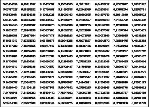
The current way of analysing motion processes normally consists of automatically recording data from motion and to collect them in files or databases. Together with the additionally recorded video pictures, one can try to find particular sequences corresponding to striking data or data series. Figure 1 illustrates that this is normally not very easy: even when it is assumed that the numbers mean positions, angles or speed, even an expert would not be able to decide whether such a series of data represents a good or a bad type of motion.

Figure 1. Part of a table of biomechanical data.

The reason for that problem is not only the amount of data but also the fact that the quality of a motion does not depend on single data on isolated points in time but on correlations of series of data over intervals of time – that is, motions build complex time-dependent patterns.

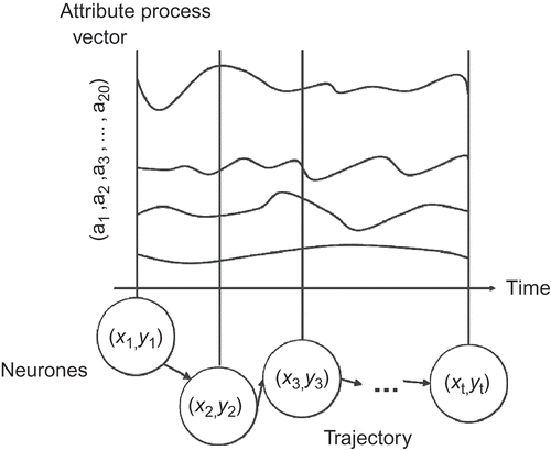
As our experience from around the last 10 years shows, such patterns can be analysed using artificial neural networks of the Kohonen Feature Map type (KFM). Figure 2 demonstrates the basic concept: at each point in time, the motion defines a set of values (e.g. positions, angles or speed of articulations) that form time-dependent vectors of attributes. These vectors can be mapped to the neurons of a network, forming a 2D representation of the high-dimensional motion.

Figure 2. Time series of motion process data, stepwise mapped to neurons of a network, generating a neuron trajectory as a 2D representation of the motion.

In the following sections, the propositions and steps that are necessary for using networks are introduced briefly.

2. Net-based pattern recognition

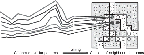
The first step of using KFM-type networks consists of training the net with characteristic information. Taking the example from Figures 1 and 2, this information can be a set of those attribute vectors that represent the situation in one point of time, each. Those attribute vectors in Figure 3 are called ‘patterns’ and are represented by the collection of curves in the left part of the Figure. According to Figure 2, during training those patterns are mapped to neurons, which are the representatives of the pattern-specific information. There are two specific properties that should be noted: Firstly, there is not just one pattern that corresponds to one neuron but a collection of similar patterns – that is, a neuron represents a type of patterns. Secondly, training does not distribute patterns all over the network but preserves the topological structure – that is, similar types of patterns correspond to neighboured neurons. Therefore, the result of training is a ‘landscape’ of neuron clusters, which form classes of types of patterns. Normally, the clusters are called ‘types’.

Figure 3. During training, patterns of data are mapped to the net, building clusters of similar types.

Note, however, that the preservation of the topological structure is just a local one: due to the fact that a high-dimensional space cannot be mapped to a 2D space smoothly, sometimes clusters that are quite dissimilar are neighboured, and sometimes clusters representing similar types are separated to quite different areas of the network. When comparing motion trajectories, this phenomenon is of importance and will be discussed in the following sections.

2.1. Trajectories

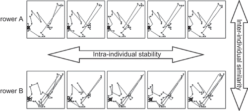
As has been explained above, the data patterns of a motion – that is, the attribute vectors – can be mapped to the corresponding neurons of a trained network where the sequence of patterns then generates a trajectory of neurons, forming a 2D representation of the motion. Figure 4 gives an example of how this can help to improve the comparative analyses of motions (see Ref. [4]): each graphic shows the trajectory of a rowing stroke of one rower. At first glance all the trajectories look quite similar. At second glance one can recognize that the strokes of the first row (i.e. rower A) are much more similar to each other than those of the second row (i.e. rower B). We therefore have two important results: there is a rather good inter-individual similarity between the strokes of rowers A and B. But the intra-individual stability of rower A seems to be significantly better than that of rower B.

Figure 4. Time series of data, as are taken from motion processes, are mapped to the corresponding neurons of a trained network, generating trajectories in form of sequences of those activated neurons.

The question is: How can we prove these statements?

The answer could be: Just measure the distance between the trajectories!

Figures 5 and 6 demonstrate what the problems are: Figure 5 shows a network with three trajectories, where the trajectories ‘black’ and ‘dark grey’ in the centre seem to be rather similar, whereas the trajectory ‘light grey’ seems to be quite different from the others.

Figure 5. Different motions build different trajectories, and it has to be decided which ones are similar or not similar to each other. The trajectories ‘black’ and ‘dark grey’ in the centre seem to be similar, whereas ‘light grey’ and ‘black’ do not.

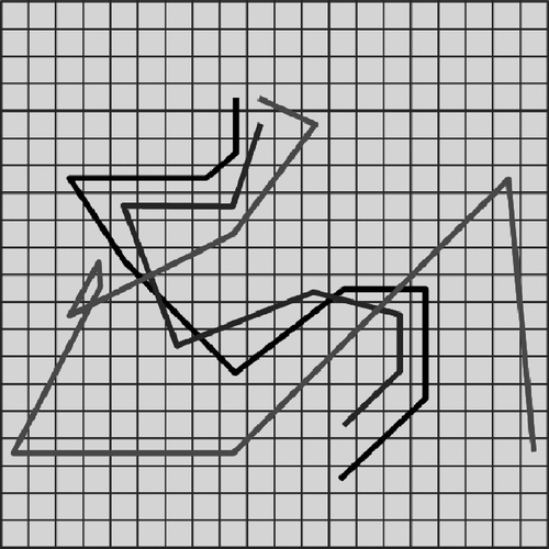
Figure 6. Using a semantic colouring for representing the types, the similarity of trajectories can be decided with respect to the sequences of types they represent. In the example the trajectories ‘light grey’ and ‘black’ are similar, whereas ‘dark grey’ and ‘black’ are not.

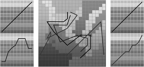
However, by taking a look at the cluster landscape of Figure 6 and projecting the trajectories stepwise to the levels of grey (i.e. ‘colours’ or types) of the respecting clusters, we get the surprising result that the light grey and the black trajectories are much more similar than the dark grey and the black ones. The reason is that Figure 5 suggests a geometrical similarity while in practice a semantic similarity, based on the colours or types of the involved clusters, is of main importance.

Following this result, the next step is to switch from the geometrical orientation of trajectories to a phase-oriented representation, which moreover is obviously more adequate to represent and analyse motions.

2.2. Phase diagrams

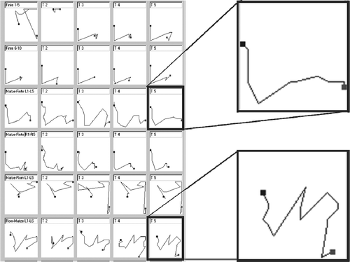
The example in this section deals with faint motions in handball. Figure 7 shows a table of trajectories, where each row shows five faints of one of six players. Like in the case of rowing from above, the question is whether the faints are similar and stable. The two enlarged examples demonstrate how difficult it would be to answer those questions by analysing only the trajectories: there are some similarities, but there also seem to be significant differences between them.

Figure 7. Faint trajectories from handball with highlighted examples in direct comparison.

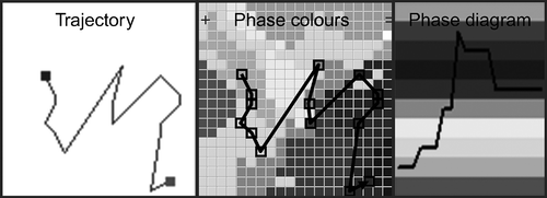
Taking phase colours in addition, as has been done in Figure 8, transforms the 2D trajectory to a 1D phase diagram, which now represents a simple time-dependent sequence of phases the motion runs through.

Figure 8. The lower faint trajectory from Figure 7 (left) transformed into a phase diagram (right) using phase colours (i.e. levels of grey).

One could argue that this might be a simplification, which is much too rough – compared with the lot of data recorded with so much effort. But, as mentioned in the introduction, the main information of a motion is not encoded in single data but in their complex correspondences, represented by such simple patterns.

Transforming the trajectories from Figure 7 into the phase colours from Figure 8 results in the phase diagrams shown in Figure 9:

Figure 9. The table of faint trajectories from Figure 7 compared with the corresponding phase diagrams to find significant similarities and dissimilarities. Highlighted are the particular examples from Figure 7.

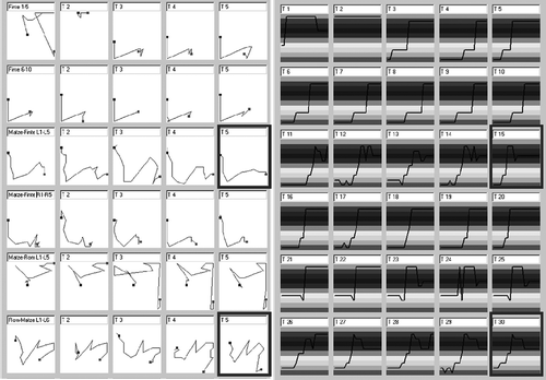
Of course, if two trajectories are quite similar to each other, the phase diagrams normally are as well. In turn, if two trajectories seem to be dissimilar, their phase diagrams can show that the motions are nevertheless similar, as examples 3 and 5 from row 5 demonstrate. Moreover, although the trajectories 3, 4 and 5 from row 1 seem to be quite similar, the phase diagrams prove that motion 4 is different from the others. Finally, the two highlighted examples from Figure 7 turn out to be more similar than expected from just the trajectories.

These results encourage us to perform the next step, namely checking the similarity of motions by measuring their distances using a further network. This could answer the question whether the marked examples from Figure 9 are of a similar type or just ‘similar in a way’.

2.3. Two-level analysis

The sequence of colours of a phase diagram can be encoded in a quite natural way using the ordinal numbers of the colours. Doing it this way, each trajectory is represented by a vector of numbers, which obviously means the same situation as at the beginning of the net-based analysis. As shown in Figure 10, this leads to a second level of analysis, where a second-level network can be trained with the phase vectors resulting from the first-level analysis.

Figure 10. Replacing the phase colours by the corresponding ordinal numbers transforms the trajectories into attribute vectors that can be taken for a net training.

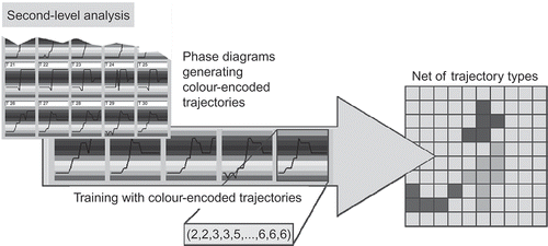
The idea is that the second-level network eventually can give information about types, similarities or stabilities of whole motions instead of just single time steps as the first-level analysis does.

The completing case study dealing with basketball free shots shall give an idea of how the different steps of analyses can work together to transfer complex information about motions.

3. Case study basketball

The project that is dealt with in the following sections was run by Andrea Schmidt from the University of Bremen, Germany, to develop methods for automatically recognizing types and measuring qualities of free shots in basketball (see Ref. [5]).

3.1. From data to trajectories

As described above, in the first analysis step the automatically recorded motion data was trained to a first-level network, which can then be used for generating and analysing free shot trajectories. Figure 11 shows this data net with an example of a free shot trajectory, which is one member of the collection of trajectories shown in the graphic on the right-hand side.

Figure 11. In the basic first step, the data net (left) generates a collection of trajectories (right).

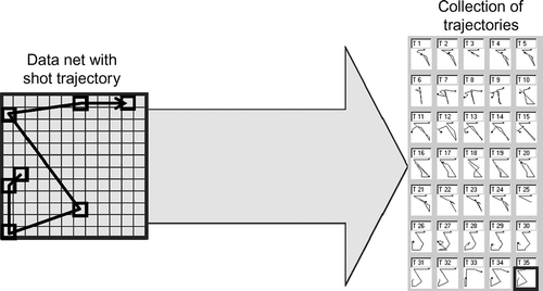
As has been discussed, above this is just a start and has to be completed by some further steps.

3.2. From data net to phase diagrams

In the second step, the neurons of the first-level data net were coloured using a combination of automatically generated clusters and expert knowledge about the phases a free shot runs through. The resulting data net with the coloured phase landscape is shown in Figure 12 (left).

Figure 12. Basic net with phase colours (left) generating phase diagrams (centre), which generate a net of shot types (right).

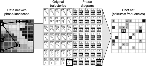
Using those phase colours, the trajectories in the third step can be transformed into phase diagrams. Trajectories and corresponding phase diagrams are shown in the middle of Figure 12. Finally, in the fourth step, the number-encoded phase diagrams can be taken for the training of the second-level shot net, which is shown on the right-hand side of Figure 12: each coloured neuron of this network represents a collection of similar diagrams. (The numbers of those neurons are not of importance for the following.) The next analysis steps are done with the second-level network.

3.3. From phase diagrams to shot-type diagrams

As has been introduced above, a major aspect of net-based analysis is to recognize the intra-individual stability and the inter-individual similarity of the players' shots. To this aim, in the fifth analysis step the neurons of the shot net from Figure 12 are coloured, following the automatically generated clusters as well as the experience of experts regarding the main types of free shot motions. The resulting net of shot types is shown in Figure 13 (right).

Figure 13. After colouring the net of shot types from Figure 12 with type colours (centre), the phase diagrams of the shots can be transferred to shot type diagrams (right), which can be taken for an easy comparison of the shot types.

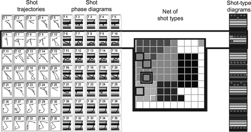
Testing – for example – the five shots of player 2 results in the five marked entries in the net of shot types, where the first light grey type differs clearly from the following four grey ones. The results of this shot typing are shown in the corresponding intra-individual stability diagrams, where the types of shots are represented in their time order. In an analogous way, the same analysis can be done with shots of different players, resulting in inter-individual similarity diagrams.

(By the way: Applying this approach to the examples from Section 2.2 (Figures 7 and 9) would show that the respective shots are not really of a similar type but just ‘similar in a way’.)

However, this type-oriented colouring of neurons is just one way of coining neurons with semantic information – which in general is called calibration and is briefly dealt with in the last step.

3.4. Multiple calibration

There are a lot of ways of calibrating the neurons of the shot net with semantic information, reaching from particular values of their corresponding biomechanical attribute vectors over properties like types or qualities of the shots up to more complex information like ‘what type of shot has what probability of success in which phase or situation of the game’. Moreover, more than one type of calibration can be used simultaneously, which then is called multiple calibration.

In Figure 14 the example of a double calibration is shown, where the neurons of the shot net on the one hand are coloured regarding the corresponding types and on the other hand regarding their expert-rated quality (which could mean here for example the quality of the motion technique or the scoring success). This is the way free shots are classified in the basketball project mentioned above. More aspects of interest could be added by just calibrating the shot net correspondingly.

Figure 14. The complete analysing process, starting with the first-level analysis resulting in phase diagrams (left), continued with generating the second-level network for trajectory typing (centre) and completed by calibrating the shots regarding types and qualities.

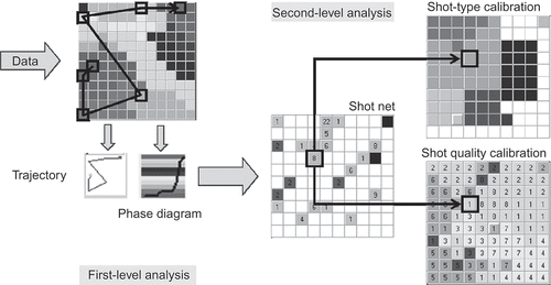
In this sixth and last step the first- and second-level networks work together in a complex database supported analysis process: controlled by an analysis schedule, the recorded source data are automatically transferred from the database to the coupled networks, where they are analysed and transformed into phase and similarity diagrams, which eventually are stored back to the database.

4. Conclusion and outlook

As has been outlined quite briefly, neural networks of type KFM can be most helpful for automatic classification of motion patterns. Besides the presented examples faints in handball and free shots in basketball, there are some more projects currently on work, like kicks in karate (working group of Kerstin Witte, University of Magdeburg), the aiming process in biathlon (working group of Arnold Baca, University of Vienna; see Ref. [6]) or the drive in golf (working group of Daniel Memmert, German Sports University (DSHS) Cologne and Ulrich Meseck, University of Bremen). Of course, not only motion processes are of interest. In the area of sport, in particular net-based game analysis is an important field where currently two projects, dealing with handball and football, respectively, are on work (see Refs. [7,8]). Finally, there are a lot of applications outside sport where net-based pattern analysis is most helpful. Some examples are fraud detection for insurances, controlling logistic processes on big airports or railway stations, or break down analyses of mobile phone communication.

It seems that we are just at the beginning of a most powerful development of net-based pattern analysis in a wide area of applications.

References

- Schöllhorn , W. and Perl , J. 2002 . Prozessanalysen in der Bewegungs- und Sportspielforschung . Spectrum der Sportwissenschaft , 14 ( 1 ) : 30 – 52 .
- Perl , J. 2004 . A neural network approach to movement pattern analysis . Hum. Mov. Sci. , 23 : 605 – 620 .
- Perl , J. 2002 . DyCoN: Ein neuer Ansatz zur Modellierung und Analyse von Sportspie-Prozessen mit Hilfe neuronaler Netze, in Sportspiele Erleben, Vermitteln, Trainieren , Edited by: Ferger , K. , Gissel , N. and Schwier , J. 253 – 265 . Hamburg : Hrsg., Czwalina .
- Perl , J. and Baca , A. Application of neural networks to analyze performance in sports . Proceedings of the 8th Annual Congress of the European College of Sport Science . Edited by: Müller , E. , Schwameder , H. , Zallinger , G. and Fastenbauer , V. pp. 342 Salzburg : Universität Salzburg, Institut für Sportwissenschaft .
- Schmidt , A. , Fikus , M. and Perl , J. 2009 . Typisierung von Basketball-Freiwürfen mit Hilfe Neuronaler Netze, in Gegenstand und Anwendungsfelder der Sportinformatik , Edited by: Augste , C. and Lames , M. 189 – 194 . Hamburg : Hrsg., Czwalina .
- Baca , A. 2008 . Informatische Methoden zur biomechanischen Analyse und Simulation . Informatik Spektrum , 31 ( 4 ) : 308 – 315 .
- Grunz , A. , Memmert , D. and Perl , J. 2009 . Analysis and simulation of actions in games by means of special self-organizing maps . Int. J. Comput. Sci. Sport 8 , : 1 22 – 37 .
- Perl , J. 2009 . “ Musteranalyse im Sportspiel mit Hilfe Neuronaler Netze, in Schriften der Deutschen Vereinigung für Sportwissenschaft ” . In Band 189 , Edited by: Lames , M. , Augste , C. , Cordes , O. , Dreckmann , C. , Görsdorf , K. and Siegle , M. 33 – 40 . Hamburg : Hrsg., Czwalina .