Flatness-based control of a horizontally moving erected beam with a point mass

Abstract

A mechanism consisting of a horizontally moving cart that carries an erected flexible beam with a point mass – as occurring in placement machines or stacker cranes – is considered. An explicitly parametrized feed-forward control law is designed using a flatness-based approach. Nominally, this control law allows one to perform fast placement motions although avoiding residual oscillations at the arrival. The efficiency of this approach and sensitivity with respect to parametric uncertainties are investigated numerically using both finite element and finite difference models. An experimental set-up is presented and some experimental results demonstrate the usefulness of the approach.

Keywords:

• Euler-Bernoulli beam; flatness; flexible robot; trajectory tracking

1. Introduction

Flexibilities of machine structures must be taken into account if high-precision and high-speed positioning is desired. Thus, the system efficiency regarding time and energy consumption can be increased by considering flexibilities in the control design instead of using a stiffer and, therefore, heavier structure.

For systems with the so-called flat or basic output, it is easy to calculate feed-forward control trajectories. For linear distributed-parameter systems, a well-developed flatness-based theory can be found in [1–4]. In the context of flexible beams, the method was applied to several problems. A first study in [5] dealt with a rotating flexible robot arm with a load at its free end (see also [6]). A corresponding experimental investigation is reported in [7] (see also [8]). The flexible arm was modelled as an Euler–Bernoulli beam there. A Timoshenko beam was studied in [9, 10]. Bending of piezoelectric actuators modelled as laminated beams was considered in [11] and the corresponding experiments are described in [12,13]. An extension to circular plates can be found in [14].

In this study, a mechanism consisting of a horizontally moving cart that carries an erected flexible beam with a point mass – the payload – is considered. Examples of such devices are placement machines or stacker cranes. For such devices, numerical approaches to the design of force trajectories that reduce residual vibrations can be found in [15,16], whereas in [17] one can find a state feedback for a strongly simplified lumped model. An input pre-shaping design is reported in [18], including the experimental results. Very interesting flatness-based results are given in [19, 20], where trajectory planning on the basis of a simplified low-order model is combined with a passivity-based feedback design and optimal motion planning is considered. Instead, in this work an exact feed-forward control law is derived from an infinite dimensional model. By taking elasticity at the clamped end of the beam into account and including the part of the beam beyond the payload the work extends [21], where the method was applied to a simplified – yet very useful – model. Moreover, in the view of parametric uncertainties occurring in practice, the parameter sensitivity and the efficiency of this approach are analysed numerically. Finally, an experimental set-up is described that was used for an experiment, results of which are given.

2. Moving beam with a point mass

The mechanism under consideration consists of a horizontally moving cart that carries an erected flexible beam with a point mass – a sketch is drawn in Figure 1.

Figure 1. Linear actuator with attached elastic structure. Elasticities of the slide bar are modelled as a rotational stiffness k. The structure between the actuator and the payload m _L as well as the structure above the load are modelled as Euler–Bernoulli beams.

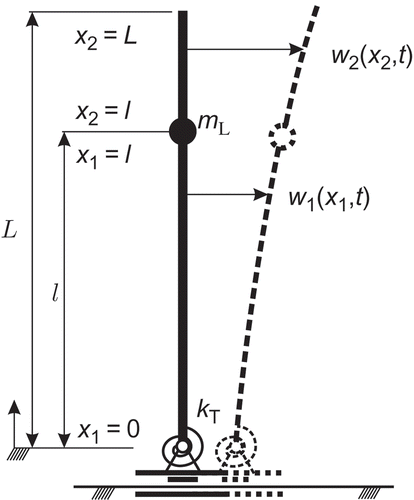
The vertical structure is modelled as an Euler–Bernoulli beam. It can be split into two sections, below and above the payload m _L. The latter is situated at a distance l from the base point. The elasticity of the slide bar (carrying the cart) is modelled as a rotational spring situated at the base point. The model of the two coupled beams leads to a boundary value problem with eight boundary conditions.

The independent variables, that is, the positions x along the beam segments as well as the time t, are normalized for the calculation:

The (normalized) partial differential equations can then be written as

(1a)

(1b)

Here, is used to denote the partial derivative whereas denotes , i = 1, 2. The (normalized) boundary conditions read as follows:

(2a)

(2b)

(2c)

(2d)

(2e)

(2f)

(2g)

(2h)

where α, φ and are defined as

Here, Equations (2a)(2a), (2e) and (2g) are the torque balances, with a spring at the base in Equation (2a)(2a). The force input appears in the force balance (2b), whereas the inertial force due to the load m_L occurs in Equation (2f)(2f), and the third force equation (2h)(2h) describes the absence of an exterior force at the free end. The remaining two conditions describe the continuity of the beam deflection and its first derivative at the intermediate point ξ = λ.

3. Flatness-based trajectory planning

It is assumed that at the beginning of the motion the mechanism is at rest:

Thus, the following ordinary differential equations can be derived from Equation (1) by the operator s for derivation w.r.t. τ (by Laplace transform or Mikusiński's operational calculus):

The following ansatz functions are chosen for and :

(3a)

(3b)

The operational functions C ₁, C ₂, S ₁ and S ₂ in Equation (3a)(3a) are defined as

(4a)

(4b)

Moreover, C⁺ , C⁻ , S⁺ and S ⁻ used in Equation (3b)(3b) are defined as

(5a)

(5b)

where

and . Here, , and denote the complex conjugates of C, S and h.

Using the ansatz (3a)(3a) and (3b) in the boundary conditions (2a), (2b), (2g) and (2h), it follows that c = αb, , f = 0, g = 0. Thus, (3a)(3a) and (3b) simplify to

(6a)

(6b)

Using Equations (6a)(6a) and (6b) in the other boundary conditions (2c)– (2f)(2f), an (inhomogeneous) linear system of equations for the four unknown parameters a, b, e and h can be derived as follows:

By determining the expressions for a, b, e and h and replacing these parameters in the solution (6a) and (6b), one obtains a representation of the form

(7a)

(7b)

This requires only elementary algebraic operations. However, the expressions are quite lengthy.

After multiplication of Equation (7a)(7a) with P ₂ and Equation (7b)(7b) with P ₁, can be eliminated, thus

(8)

Here, a new ‘free parameter’ is introduced:

(9a)

(9b)

(9c)

This new variable is called a flat (or basic) output of the system [1]. Use of this flat output would allow one to parametrize the complete system trajectories.

However, a slight simplification results by parametrizing trajectories of the lower beam only. To this end, one may introduce

(10)

It is obvious from Equations (9a)(9a) and (9c) that this allows one to parametrize trajectories of w ₁ and . This is done in the sequel.

The calculation is quite similar to what is done in [1,5]: a series expansion of the (transcendental) operational functions involved in the expressions of P ₁ and Q ₁ is derived from the series representations of the hyperbolic functions. After sorting and interpreting s as differentiation w.r.t. time, the beam deflection w ₁(ξ, τ) is obtained as a series

(11)

Similarly, the actuator force results as

(12)

Here, the coefficients in Equation (11)(11) read

and those in Equation (12)(12) are given by

4. Parametrization of the flat output trajectory

According to the preceding discussion, the motion can be parametrized by choosing the trajectory of the flat output y. For instance, rest to rest motions or accelerations can be described.

To satisfy the homogeneous initial conditions and to guarantee series convergence, trajectories are chosen in such a way that the following conditions are met [1]:

•	is a ∞ function,
•	for t ≤ 0, i ≥ 0,
•	for t ≥ T, i ≥ 0,
•	y is a Gevrey function of class α < 2, that is, a ∞-function of the real variable t such that for each closed interval one has with real constant parameters α, m, and γ depending on K [1].

The convergence of the series for trajectories satisfying these conditions is a direct consequence of the fact that the operators involved are obtained by multiplying the elementary operators introduced in Equations (4) and (5) and powers of s – see, for example, [1,5] for further details.

As a result of the fact that the derivatives of y should vanish at the beginning and at the end of a transition, the function y must be smooth and cannot be an analytical function unless it is identical to 0. An appropriate choice of y can be achieved using

(13)

with , . This function is smooth and it is a Gevrey function of class (see [22]). An alternative would be [3]

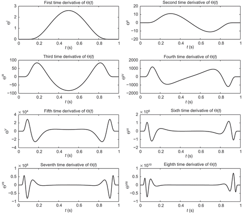
For illustration of the properties of the trajectory chosen, Figure 2 shows the first eight time derivatives of Θ from Equation (13)(13) with σ = 1.1 and T = 1.

Figure 2. Time derivatives of the Gevrey function used.

4.1. Parametrization for positioning

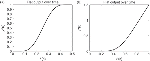
For positioning purposes, the target trajectory (to be met after t = T) is simply a constant . It describes the span of the desired motion. A trajectory meeting the conditions listed above is obtained by scaling the one in Equation (13)(13) by the constant parameter :

(14)

A graph of such a function is drawn on Figure 3(a).

Figure 3. Flat output trajectories for positioning (a) and acceleration (b) purposes.

4.2. Parametrization for acceleration

If positioning over longer distances is required, the maximum velocity of a drive will set additional limits. It is desirable to be able to accelerate the device to maximum speed, yet in such a way that no residual vibration appears after an acceleration process has finished [23]. For this task, the target function is defined by

One possible choice for the trajectory is

and then

to meet the condition . A graph is depicted on Figure 3(b).

4.3. Parameter sets of example systems

In the following sections, the feed-forward control law is applied to a laboratory set-up and a set of parameters that may correspond to a huge device like a stacker crane. Corresponding parameters are given in Table 1. To demonstrate the industrial relevance of the results, numerical studies of the parameters of a large-scale device (LSD) are presented. In addition, experimental results obtained with a laboratory set-up Linearly Actuated Robot System (LARS) are presented below, and the corresponding parameters are given in the same table, for the sake of clarity.

Table 1. Parameter sets of the laboratory set-up LARS and an LSD

Name of parameter	Symbol	Unit	LARS	LSD
Modulus of elasticity	E	N/m^2	21 × 10^10	7.155 × 10^10
Second moment of area	I z	m^4	90 × 10^−12	5.993 × 10^−5
Cross-sectional area	A	m^2	12 × 10^−5	6542 × 10^−6
Density	ρ	kg/m^3	7850	2740
Length of beam	L	m	0.6	10
Rotational stiffness of clamping	k	Nm/rad	4.63 × 10^7	2.15 × 10^6
Mass at the foot point	m	kg	3.659	320
Mass of load (m T + m Z)	m L	kg	max. 2.138	max. 110

4.4. Motion planning results

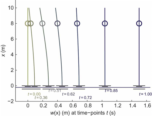
The planning results that can be achieved for a highly dynamic positioning of a device using the analytical planning algorithm proposed are shown in six figures. The trajectories of y used for positioning and acceleration are depicted in Figure 3. The field of deflection plotted over time t is given in Figures 4 and 6, whereas the snapshots of the system during a planned motion are shown in Figures 5 and 7.

Figure 4. Field of beam deflection over time.

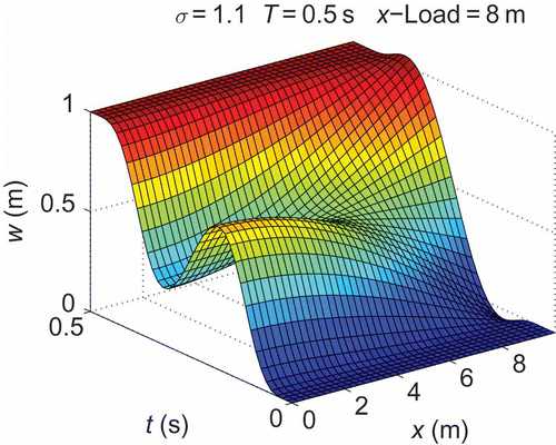
Figure 5. Phases of positioning movement.

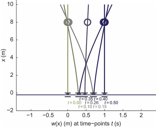
Figure 6. Field of beam deflection over time.

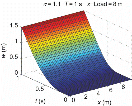
Figure 7. Phases of acceleration to a speed of 3 m/s.

5. Simulation model and results

A quite extensive simulation study has been conducted using different models and different finite dimensional approximations. This allows one to gain valuable insight into the usefulness of the approach. In particular, such simulations are used to study the influence of parametric uncertainties on the tracking results achieved in open loop.

5.1. Using a finite difference model

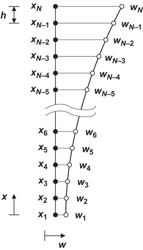
One simplified continuous mechanical model is shown in Figure 8. Here, the payload m_L is attached to the beam through a linear spring with stiffness c _TCP in the horizontal direction. With this, effects of flexibilities in the payload carriage can be studied. Note that moments of inertia caused by the payload are neglected. Indeed, for mechanisms built of two pylons these are irrelevant. For systems consisting of a single beam, it must be verified whether neglecting the payload moment of inertia is appropriate. From such a simplified model, a finite dimensional approximation is readily obtained by spatial discretisation of the Euler–Bernoulli beam using finite differences, as indicated in Figure 9. Furthermore, the discretized model can also be used for the design of a controller and an observer. A low number of nodes may be sufficient to this end (six nodes being used in experiments reported below).

Figure 8. Continuous model.

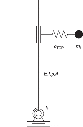
Figure 9. Discretized model of the beam.

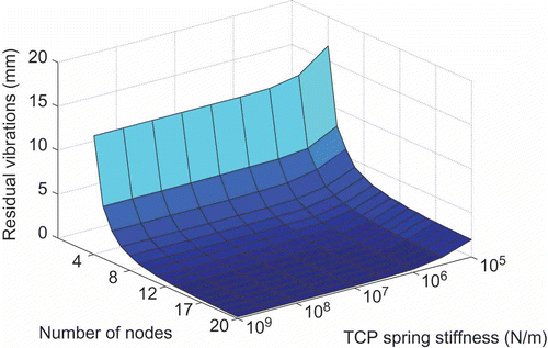
In Figures 10–12 the amplitudes of the residual vibrations at the free and the clamped ends, as well as at the tool center point (TCP), are drawn as functions of the stiffness c _TCP. The TCP is the point on the beam where the payload is attached. Its coordinate is x = l (which means ξ = λ) and the deflection is w(l, t). For a high spring stiffness, the magnitude of the residual vibrations is a measure of the error introduced by the discretization. In the view of these results, in the numerical studies discussed in the next section, 20 nodes have been used.

Figure 10. Vibration amplitudes at the top of the beam.

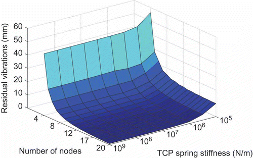
Figure 11. Vibration amplitudes at the TCP.

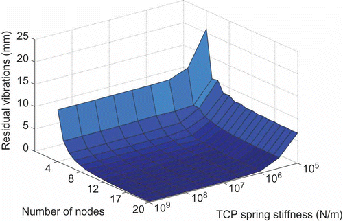
Figure 12. Vibration amplitudes at the bottom of the device.

5.2. Parameter variations

The influence of parameter uncertainties on the motion-planning approach has been investigated numerically. As an example, two different actuator force trajectories generated by the flatness-based trajectory planning are considered here – for a transition time of 1 and 2 s, respectively. Both are designed in such a way that the available actuator force amplitude is used.

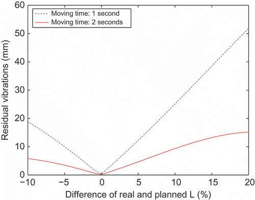
In Figure 13, the amplitudes of residual vibrations are given for different TCP heights and several transition times. It is obvious that the sensitivity w.r.t. parameter variations decreases with longer transition times. In Figure 14, the payload m_L is varied and Figure 15 shows a variation of the beam length.

Figure 13. Variation of the TCP height.

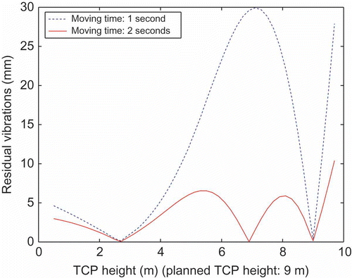
Figure 14. Variation of the payload from 0 kg up to 100 kg.

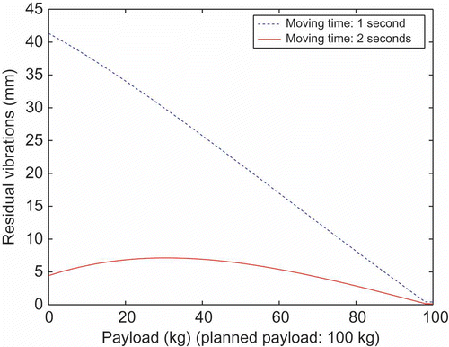
Figure 15. Variation of the beam length.

In Figure 16, the sensitivity w.r.t. variations of the bending stiffness EI is shown. Similarly, Figure 17 concerns the beam mass ρA, and Figure 18 the rotational stiffness k. It can be seen that amplitudes of residual vibrations (>10 mm) occur for deviations of more than 15% of the nominal parameters.

Figure 16. Variation of the bending stiffness EI.

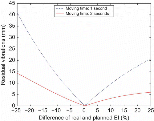
Figure 17. Variation of the beam mass ρA.

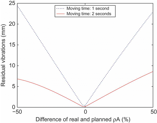
Figure 18. Variation of the rotational stiffness k.

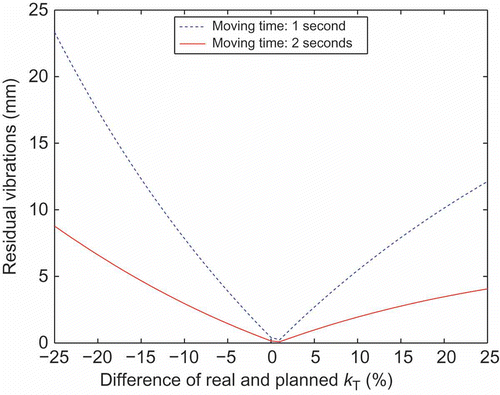
Two particularly interesting conclusions can be drawn from the parameter studies. Regarding the position of the payload in Figure 15, residual vibrations can be avoided for a specific force trajectory with different TCP heights. Moreover, for a given acceptable limit of residual vibrations, a limit of allowable parameter variations can be given. For the LSD with a height of 10 m, a limit of an amplitude of 5 mm would be acceptable and, therefore, parameter variations of at least 5% could be admitted.

6. Experiments

To be able to verify the theoretical results, a laboratory set-up (LARS) was designed at the Chair of Applied Mechanics at Technische Universität München. The aim in using this set-up is to demonstrate highly dynamic positioning.

6.1. Mechanical design

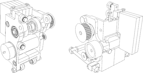
The wagon moving along the beam consists of two symmetric parts, as depicted in Figure 19. Steel wheels are coated with rubber to get a high friction coefficient. Each wagon can carry up to five additional loads. The mass of the wagon is 1560 and 2190 g including the additional loads. Motors are designed to realize accelerations of two times gravity for a wagon with full load.

Figure 19. 3D sketch of the wagon moving along the beam.

The mechanical properties relevant to the control design for flexible systems are the cross-section and the bending stiffness. These correspond to the cross-section and the material properties. A rectangular section of 3 mm × 40 mm has been chosen (3 mm in the direction of the motion).

Another aspect to be taken into account in such a design is the desire to have the beam aligned along the vertical when at rest. Together with the maximum weight of the wagon, the following calculation allows one to guarantee a single stationary bending line, the vertical one.

With the force F _q acting normal to the line of deflection at the free top of the beam, the line of deflection satisfies

(15)

Integration yields

(16)

Specifically, at the top of the beam one has

(17)

With the angle of deflection φ at the top , whence

(18)

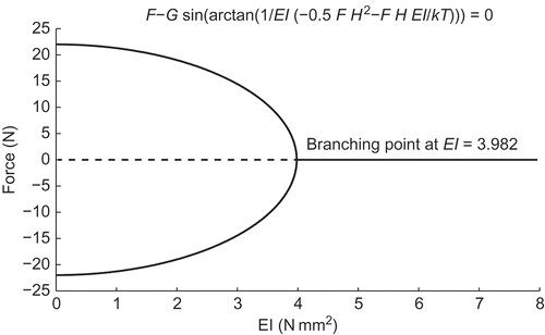
With the geometry of the normal force and the gravitational force G = m _Lg of the load at the end of the beam, F _q = G sin (φ), one obtains the implicit equation

(19)

Figure 20 shows the solutions. With the parameters used for LARS, one has a safety factor larger than 4.5.

Figure 20. Branching of the solution of implicitly given equilibrium condition.

6.2. Actuator

Fast dynamics, large peak forces and low force ripples are desired in a laboratory set-up. Therefore, a permanent magnet synchronous linear motor has been chosen. In Table 2, the most important parameters of the actuator are given.

Table 2. Parameters of the coreless linear synchronous motor used

Name	Symbol	Value
Nominal force	F N	90 N
Peak force	F S	270 N
Maximum speed	v S	5 m/s
Maximum acceleration	a max	100 m/s^2
Sensor accuracy	x abs	±0.02 mm
Sensor resolution	x res	±0.001 mm
Time constant of current controller	T Cur	0.4 × 10^−3 s

The sensor system is a magnetic position measurement system with an analogue sin/cos output. The given sensor resolution is limited by the high frequencies of the resulting incremental encoder signal. Due to the low-pass character of the cables, higher resolution may result in the loss of position ticks at high speed.

6.3. Friction identification

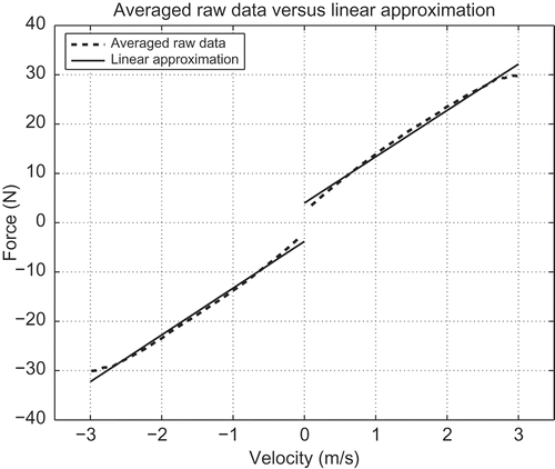
Having a very accurate actuator with excellent dynamic performance is not enough. Friction has to be taken into account, too. Therefore, for friction compensation an off-line friction identification has been performed. To this end, a state machine has been implemented, sampling the bearing friction at different speeds and directions. A classical speed controller has been used. After a period corresponding to five times the time constant T _S of the designed speed controller, the desired speed is assumed to be reached. Measurements are taken into account only after this transition period. The measurement of the required force has been repeated five times for each considered value of the speed, and averaged as shown in Figure 21. The result has been approximated by two straight lines, for the positive and the negative part of the curve, by a least squares approximation. Because Stribeck-like effects could not be observed (with the equipment used), these effects were neglected.

Figure 21. Raw data versus friction approximation using least squares.

6.4. Structure of the controller

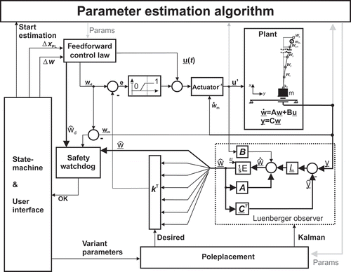
The main ingredient of this approach is the flatness-based feed-forward control that, nominally, allows one to achieve positioning and acceleration without residual vibrations. It is advisable to complete such open-loop control with a friction compensation and a feedback loop. The latter is activated at the end of the motion only and its role is to tackle small residual oscillations occurring due to various imperfections. Many different approaches would be possible. Here, a standard linear quadratic regulator design based on a discretized model with six nodes was used in the experiment. This choice was made after simulation studies with different parameter sets. Finally, fine tuning was made on the experimental set-up.

A schematic representation of the complete controller structure used is depicted in Figure 22. In the experiment, the controller was activated with a linearly increasing weight on a small interval after 0.9 times the transition period only. Friction compensation and an observer, with a small dead zone around zero velocity, were active during the entire motion.

Figure 22. Controller structure.

6.5. Experimental results

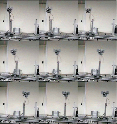
In the following, some experimental results are reported. With the set-up described above, a rest to rest manoeuvre within 0.6 s has been performed. The 2.183 kg payload has been fixed at a height of 0.5 m. The feedback controller was activated at the end of the motion, as described above. The field of deflection observed with the Luenberger observer is illustrated in Figure 23. Snapshots taken from a movie of the manoeuvre are given in Figure 24. Without the feedback, only very small oscillations occur, as compared to a simple PID-position controller (neither one reported here). Regrettably, at present on LARS no measurement of the deflection is available. However, the observer states that representing the deflections at the six nodes considered as depicted in Figure 23 confirms the result.

Figure 23. Field of deflection during a positioning manoeuvre.

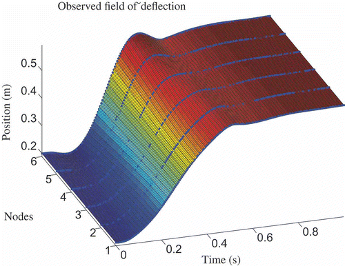
Figure 24. Phases of a motion over a distance of 0.4 m in 0.6 s.

7. Conclusion

Using the flatness-based motion planning approach presented, positioning with very low residual vibrations can be performed. Parametric uncertainties, specifically on the payload and its height, have been investigated numerically. (These results have been confirmed by experiments not reported here.) Compared to standard trajectories of today's drives, experimental results are very good even with large parameter variations. As a consequence, with such type of feed-forward control highly dynamic positioning of lightweight (elastic) structures seems becoming possible.

References

- Rudolph , J. 2003 . Flatness Based Control of Distributed Parameter Systems , Aachen : Shaker Verlag .
- Woittennek , F. 2007 . Beiträge zum Steuerungsentwurf für lineare, örtlich verteilte Systeme mit konzentrierten Stelleingriffen , Aachen : Shaker Verlag .
- Rudolph , J. , Winkler , J. and Woittennek , F. 2003 . Flatness Based Control of Distributed Parameter Systems: Examples and Computer Exercises from Various Technological Domains , Aachen : Shaker Verlag .
- Meurer , T. 2005 . Feedforward and Feedback Tracking Control of Diffusion-Convection-Reaction Systems using Summability Methods , Düsseldorf : Fortschritt-Berichte VDI Reihe 8 Nr. 1081, VDI-Verlag .
- Fliess , M. , Mounier , H. , Rouchon , P. and et Rudolph , J. Systèmes linéaires sur les opérateurs de Mikusiński et commande d'une poutre flexible, ESAIM Proceedings , 2 (1997) 183 – 193 .
- Lynch , A.F. and Wang , D. 2003 . “ Flatness-based motion planning control of an Euler–Bernoulli beam in a gravitational field ” . In Algebraic Methods in Flatness, Signal Processing and State Estimation , Edited by: Sira-Ramirez , H. and Silva-Navarro , G. 149 – 170 . Innovación Editorial Lagares Mexìco .
- Aoustin , Y. , Fliess , M. , Mounier , H. , Rouchon , P. and Rudolph , J. Theory and practice in the motion planning and control of a flexible robot arm using Mikusiński operators . Proceedings of the 5th Symposium on Robotics and Control . Nantes, France. pp. 287 – 293 .
- Hisseine , D. , Lohmann , B. and Kucynski , A. Two control approaches for a flexible-link manipulator . Proceedings of IASTED, International conference on Robotics and Applications, RA’99 . Santa Barbara, CA.
- Rudolph , J. and Woittennek , F. 2003 . Flachheitsbasierte Steuerung eines Timoshenko-Balkens . ZAMM , 83 : 119 – 127 .
- Woittennek , F. and Rudolph , J. 2003 . Motion planning and boundary control for a rotating Timoshenko beam . PAMM , 2 : 106 – 107 .
- Rudolph , J. and Woittennek , F. Flachheitsbasierte Randsteuerung von elastischen Balken mit Piezoaktoren . at-Automatisierungstechnik , 50 ( 2002 ) 412 – 421 .
- Haas , W. and Rudolph , J. Steering the deflection of a piezoelectric bender . Proceedings of the European Control Conference ECC 99 . Karlsruhe. No. F1010-4
- Meurer , T. , Thull , D. and Kugi , A. 2008 . Flatness-based tracking control of a piezoactuated Euler-Bernoulli beam with non collocated output feedback: theory and experiments . Int. J. Control. , 81 : 475 – 493 .
- Woittennek , F. and Rudolph , J. 2004 . Motion planning for a circular elastic plate . PAMM , 4 : 149 – 150 .
- Bachmayer , M. , Zander , R. and Ulbrich , H. 2009 . Numerical approaches for residual vibration free positioning of elastic robots . Materials Sci. Eng. Technol. , 40 : 161 – 168 .
- Schuhmacher , M. 2001 . Untersuchung des Schwingungsverhaltens von Einmast-Regalbediengeräten , Dissertation Universität Karlsruhe (TH), Institut für Fördertechnik und Logistiksysteme .
- Dietzel , M. 1999 . Beeinflussung des Schwingungsverhaltens von Regalbediengeräten durch Regelung des Fahrantriebs , Dissertation, Universität Karlsruhe (TH), Institut für Fördertechnik und Logistiksysteme .
- Park , S. , Kim , B.K. and Youm , Y. 2001 . Single-mode vibration suppression for a beam-mass-cart system using input preshaping with a robust internal-loop compensator . J. Sound Vibration , 241 : 693 – 716 .
- Ennsbrunner , H. and Schlacher , K. Control of weakly damped finite and infinite dimensional Euler–Lagrange Systems . Proceedings of the 16th Conference of the International Federation of Automatic Control . Prague.
- Staudecker , M. , Schlacher , K. and Hansl , R. Passivity based control and time optimal trajectory planning of a single mast stacker crane . Proceedings of the 17th World Congress of the International Federation of Automatic Control . Seoul.
- Bachmayer , M. and Ulbrich , H. Trajectory planning for linearly actuated elastic robots using flatness based control theory . Proceedings of the 12th International Conference of Theoretical and Applied Mechanics . Adelaide.
- Lynch , A.F. and Rudolph , J. 2002 . Flatness-based boundary control of a class of quasilinear parabolic distributed parameter systems . Int. J. Control. , 75 : 1219 – 1230 .
- Bachmayer , M. , Rudolph , J. and Ulbrich , H. Acceleration of linearly actuated elastic robots avoiding residual vibrations . Proceedings of the 9th International Conference on Motion and Vibration Control . Munich.