Genetic algorithm approach with frequency selectivity for model order reduction of MIMO systems

Abstract

A novel genetic algorithm (GA) approach with frequency selectivity advantage for model order reduction (MOR) of multi-input–multi-output (MIMO) systems is presented in this article. Motivated by singular perturbation and other reduction techniques, the new MOR method is formulated using GAs, which can be applied to single-input–single-output (SISO)- or MIMO-type systems. The GA procedure is based on maximizing the fitness function corresponding to the response deviation between the full-order model and the reduced-order model with the option of substructure preservation. The proposed GA-MOR method is compared to the well-known reduction techniques, such as the Schur decomposition balanced truncation, proper orthogonal decomposition (POD) and state elimination through balancing-related frequency-weighted realization in addition to other recent methods. Simulation results validate the superiority and robustness of the new MOR technique as it can search the solution space for almost optimal solutions.

Keywords:

• genetic algorithms
• balanced realization
• MOR
• POD
• Schur decomposition

1. Introduction

In system modelling, the mathematical procedure often deals with many system details presented in the form of high-order differential equations. These equations lead to a high-order mathematical model. In control system design, it is usually preferable to obtain a reduced-order model that adequately describes the significant dynamic behaviour of the high-order system. In recent years, model order reduction (MOR) has come to be viewed as a method for generating compact models from all sorts of physical system modelling tools [1–3 3]. MOR has received the attention of many researchers because model reduction would lead to cost minimization, whereas detailed modelling would be practically too demanding [4]. In control system, because feedback controllers do not usually consider all the dynamics of the system, MOR becomes a very important issue [5–7 7].

For MOR, there are different scenarios that can be performed. One scenario obtains reduced models that are completely new and not related to the original models, in terms of their critical frequencies of either single-input–single-output (SISO) or multi-input–multi-output (MIMO) systems. On the contrary, another scenario obtains reduced models that preserve the important properties of the original system, such as dominant frequencies of either SISO or MIMO systems. It is to be noted that the later scenario is more preferable, if possible, due to its meaningful physical interpretation in obtaining similar models and due to minimum changes in the original systems [8,9].

The MOR problem has been investigated in literature extensively. Willcox and Perarie [10] proposed an algorithm to reduce the model order using the proper orthogonal decomposition (POD) analysis of the primal and dual systems, low-rank, reduced-range approximations to the controllability and observability gramians. Fujimoto and Scherpen [11] proposed a singular perturbation type balanced realization and model reduction for discrete non-linear dynamical systems based on Hankel singular value analysis, which preserves the related controllability and observability properties. Heydari and Pedram [12] proposed a spectrally weighted balanced truncation technique for tightly coupled integrated circuit (IC) interconnects, when the interconnected circuit parameters change because of statistical variations in the manufacturing process. Rabiei and Pedram [13] proposed a method that uses the truncated balanced realization technique as well as the Schur decomposition to develop an efficient numerical method for the order reduction of linear time invariant (LTI) systems. Gugercin et al. [14] proposed an iterative rational Krylov approach (IRKA) for optimal H₂ model reduction. Their approach is concerned with SISO-type systems only and is based on minimizing the H₂-norm. This minimization leads to a non-convex problem that can get stuck at local minima and hence optimality will not be achieved [15]. Recently, Parmar et al. [16] proposed a reduction method with pole centroid retaining in the reduced model. Their method deals with SISO systems only. In addition, it works for real poles only.

Genetic algorithm (GA)-based MOR, on the contrary, has received some of the researchers' attention as well. Recently, Panda et al. [17] employed a particle swarm optimization technique to obtain a reduced-order model of SISO large-scale linear systems. Their technique is based on integral square error (ISE). Vishwakarma and Prasad [18] proposed a mixed method for reducing the order of large-scale linear systems. They have synthesized the denominator of the reduced-order transfer function (TF) using modified pole clustering, whereas the coefficients of the numerator elements are computed using GA. Parmar et al. [19] presented a technique for MOR using GA for SISO linear time systems. They have focused on obtaining a reduced-order model that maintains stability and retains the steady-state value.

Despite having several reduction methods, no approach always provides the satisfactory results for all systems [16]. Hence, in this article, we propose a new technique for MOR of dynamical control systems using GAs with frequency selectivity, whereas it may be applied without frequency restrictions. The proposed technique has been compared to some of the well-known methods that are based on the system transfer behaviour, namely, the balanced gramian-based POD technique [6,10], the frequency-weighted balanced realization technique [11] and the Schur decomposition balanced truncation technique [13,20]. In addition, the new method has also been compared to some other recent and older techniques [16,21–24 24].

The organization of this article is presented as follows. Section 2 presents a background for the MOR. In Section 3, GA procedure for MOR is presented. The practical implementations of the GA-based MOR along with simulation comparative results of different MOR techniques are presented in Section 4. The conclusion is presented in Section 5.

2. Background

Consider the following nth-order LTI system:

(1)

(2)

where is a state vector; and contain the inputs and outputs, respectively. A, B, C and D are matrices with appropriate dimensions. The objective of the reduction is to obtain an n_r th-order reduced model (n_r < n), which can mimic the behaviour of the original full-order model. A two-time-scale class of model reduction methods can be interpreted as performing a similarity transformation P yielding the partitioned forms [25]:

(3)

As a projection-based method, by considering the states in vector x ₂ unimportant (explicitly set to zero), the reduced model is defined as

(4)

When writing the similarity transformation P as [25]

(5)

the projection on T along L is TL and the reduced model is then given by [25]

(6)

where L and T are called truncation matrices.

The partitioned forms in Equation (3)(3) can also be used to construct the singular perturbation approximation (SPA), also known as the state residualization. As a non-projection method, the state residualization method sets the derivatives of the states in vector x ₂ to zero. After eliminating the vector x ₂, the following reduced model is obtained:

(7)

For better model reduction, the state residualization method may use the gramian-based balancing technique. The balancing process is achieved by obtaining the gramians of the state space and performing state-space transformation. This transformation is required to obtain the gramians with r small diagonal entries. The reduced model order may then be obtained by eliminating the last r states. This can be performed using MATLAB functions.

An important similarity transformation can be obtained using the Schur decomposition or Schur triangulation [13,20]. This form of transformation states that if the matrix A is an (n × n) square matrix with complex entries, then A can be expressed as

(8)

where P is a unitary matrix (P ⁻¹ = P*) and is an upper triangular matrix, which is called the Schur form of A. Balancing and using the unitary matrix P, a complete system transformation and model reduction may be obtained. It is well known that the Schur decomposition is not unique. This fact has led for different research investigation and implementation of the Schur formulation [25–27 27].

The well-known POD method has also been used for MOR [6,10,28]. It involves the calculations of the eigenvalue decomposition of a data covariance matrix. In this method, it is assumed that the system in Equation (1)(1) can be either observed (measured) for various inputs at different times or simulated. Then, define [29]

as an (n × z) matrix whose columns are these spatial snapshots. Now, the singular value decomposition (SVD) of Γ is given by

where P and N are orthogonal matrices and Σ contains the singular values σ _i in its diagonal sorted in a descending order of magnitude. If the SVD truncation is desired at the n_r term (n_r < n), then the truncation of the left singular vectors of Γ is given as P _r . Hence, the state vector in Equation (1)(1) can be written as [29]

(9)

which leads to the formulation of the n_r th-order reduced model:

(10)

In steps, this is performed as follows [29]:

1. Run s full simulations with the same spatial mesh (i.e. changing the source location).

2. Extract k snapshots from each simulation, for a total of columns in Γ.

3. Calculate the SVD of Γ.

4. Truncate at level p < 1, where p corresponds to a certain fraction of the total information to be preserved.

5. With the resulting r modes construct the reduced-order model as shown in Equation (10)(10).

3. Genetic algorithms

GAs can be distinguished from calculus-based and enumerative methods for optimization in many different ways [30,31]. GAs search for optimal solutions using a population of individuals. The population-based nature of GAs gives them two major advantages over other optimization techniques. First, it identifies the parallel behaviour of GAs that is realized by a population of simultaneously moving search individuals or candidate solutions [30,31]. Implementation of GAs on parallel machines, which significantly reduces the CPU time required, is a major interesting benefit of their implicit parallel nature. Second, information concerning different regions of solution space is passed actively between the individuals by the crossover procedure. This information exchange makes GA an efficient and robust method for optimization, particularly for the optimization of functions of many variables and non-linear functions.

On the contrary, the population-based nature of GAs also results in two main drawbacks. First, more memory space is occupied; that is, instead of using one search vector for the solution, several search vectors are used which represent the population size. Second, GAs normally suffer from computational burden when applied on sequential machines. This means that the time required for solving certain problems using GAs will be relatively large, where the solution time is a major point when we are interested in real-time applications. However, if off-line solutions are required for any practical problem, then our major concern will be the solution accuracy rather than the time required for the solution. In this article, we present the GA-MOR as an off-line operation where the objective is accuracy.

The fact that GAs use only objective function information without the need to incorporate highly domain-specific knowledge points to both the simplicity of the approach and its versatility. This means that once a GA is developed to handle a certain problem, it can easily be modified to handle other types of problems by changing the objective function in the existing algorithm. This is why GAs are classified as general-purpose search strategies.

The stochastic behaviour of GAs cannot be ignored as it is a main part that gives them much of their search efficiency. GAs employ random processes to explore a response surface for a specific optimization problem. The advantage of this type of behaviour is the ability to escape from local minima without supervision [31].

In this article, as shown in Figure 1, the GA is performed based on the following operations [31]:

Figure 1. Block diagram of the GA procedure.

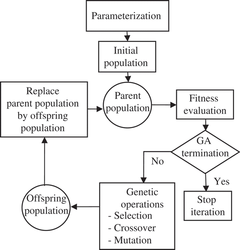
1. Parameterization: In this step, the number of parameters that the GA would have to estimate is determined. Consider reducing the system in Equation (1)(1) to the following reduced-order model:

   (11)
   (12)
   where , and . Please note that the feed-through Du(t) has been eliminated to produce a strictly proper model. For the case of frequency selectivity, the number of parameters that have to be estimated by the GA is given by
   (13)
   where A_r is set in the modal form (diagonal matrix) with retained selected frequencies and only the elements of B_r and C_r to be estimated. On the contrary, if the proposed GA is to be applied without frequency selectivity, as will be shown in Example 3, then the matrix A_r will also have to be estimated by the GA. Hence, Equation (13)(13) will then be modified as follows:
   (14)

   The GA type used in this article is a binary GA, where each value in the solution set consists of a number of bits (genes). The number of bits used to encode each parameter depends on three variables: lower parameter bound (p _l), upper parameter bound (p _u) and quantization level (φ). Hence, the number of bits used is defined as [32]

   (15)

2. Initialization: Based on the number of unknown parameters (n_p ), the GA creates an initial population of individuals (chromosomes) or solutions, which are rows in the population matrix. Each individual contains n_p parameters. Given that each parameter value consists of n _bits number of bits, each solution set (row or individual) will consist of a total number of bits given by . Hence, for a population size (n _pop), the entire population matrix will have a bit size of (n _pop × n _b,t) or element size of (n _pop × n_p ), as shown in Figure 2 for a parameter with five bits randomly generated. These genes can be later decoded back into decimal values, which provide the desired parameters' values.

3. Evaluation: The solution sets are each taken to have their fitness evaluated, upon which later procedures are based on. The fitness evaluation process is performed by distributing the elements of the chromosome as values of the unknown parameters in the B_r and C_r matrices. Next, the newly obtained system is simulated to produce an estimated output (y_r ). This output is subsequently compared with the output of the original system (y) giving the fitness for this solution set as follows [33]:

   (16)
   where
   (17)
   where N is the number of elements in the output vector(s). The higher this fitness is, the closer the reduced model is to mimic the original model. The fitness value will come to define later processes such as crossover, elitism and replacement. This same fitness evaluation process is performed for every chromosome in the GA population at each generation.

4. Selection: In the selection process, chromosomes are chosen from the current population to produce new offspring for the next generation. The larger the fitness value of a chromosome, the higher the probability of the chromosome to contribute one or more offspring to the next generation. The population fitness and the associated chromosomes are ranked from highest fitness to lowest fitness. Based on a rank ratio, only the best chromosomes are selected to continue to the crossover process, whereas the rest are left. Deciding on how many chromosomes to keep is somewhat arbitrary. In the proposed algorithm, a chromosome random pairing with an initial selection rate X_r  = 0.65 was used and the top 65% fitness chromosomes were placed to produce new solutions for the next generation.

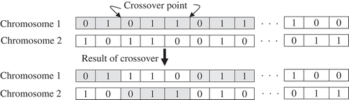
5. Crossover: In the crossover operation, a pair of chromosomes is mated, based on random pairing selection, to produce two offspring. The two parent chromosomes are crossed over at random points to segment each chromosome into a number of parts. These parts of each chromosome pair are swapped between each other to produce two new chromosomes, the offspring. This is shown in Figure 3 for a general crossover operation. Crossover is not applied to all pairs of chromosomes selected for producing new solutions. For every parent chromosome pair, a crossover rate decides whether crossover occurs. If crossover is not applied, children are produced simply by duplicating the parents. This gives each chromosome a chance of passing on its genes without the disruption of crossover. In the proposed algorithm, the crossover rate is set to 0.85, meaning that 85% of parent pairs produce offspring. The number of crossover points for the parent chromosomes is chosen randomly for each generation.

6. Mutation: Mutation operation is applied to guarantee that the offspring will have new qualities and to provide a small amount of random search to guard against premature convergence. Mutation is applied to each offspring individually after crossover, where it randomly flips any bit (gene) with a small mutation probability (between 0.1 and 0.001). In the proposed methodology, the mutation rate is set to 0.0125.

7. Replacement: Replacement operation takes place once the crossover of all parent chromosome pairs is performed. The decision on which offspring replaces which population individual is made based on the fitness evaluation. Fitness is evaluated for all the resulting offspring as well as for all of the original population individuals and a replacement factor decides how many of the offspring with the highest fitness values are to replace the main population individuals. In the proposed algorithm, a replacement factor of 0.70 is used; in other words, 70% of the original population will be replaced by the best chromosomes in the offspring population. This process continues until reaching the end of the population size or the best desired fitness.

8. Termination: Termination is performed when some convergence criterion is met, such as the best individual fitness value found to exceed a threshold or a maximum number of generations is reached. After terminating the algorithm, the optimal solution of the problem is the best individual so far found. Depending on the GA's termination condition, the algorithm will stop to provide its best results. The termination condition for the proposed algorithm is reaching a fitness value of 99.999% and an average fitness value of at least 99.9% in the entire population set. When the algorithm terminates, the highest fitness chromosome is distributed across the B_r and C_r matrices to produce the required values of the reduced-order model.

Figure 2. A population matrix of n _pop chromosomes and n_p parameters.

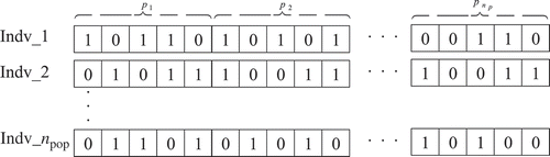
Figure 3. Random crossover operation for a general chromosome.

4. Results and discussion

To demonstrate the proposed method of GA-MOR, we will consider different dynamical models and show the differences of our new method compared to other existing methods.

4.1. Example 1

A two-area power system is considered in this example [34]. The system is a seventh-order model with two inputs and two outputs. The state vector is given as follows:

where f ₁ and f ₂ are the frequencies, P _t1 and P _t2 are the turbine powers, P _u1 and P _u2 are the governor states at area one and area two correspondingly and P _tie is the transferred power between the two areas. The system matrices are [35]

with system frequencies [36] λ = {–0.5532 ± 3.1342i, −0.8701 ± 1.3728i, −3.0484, −12.5882,−13.277}. For MOR with frequency selectivity, the reduced-order model state matrix A_r is set in the modal form where all of the selected complex frequencies [36] (because they are the dominant) are placed on the diagonal. The GA-MOR technique, on the contrary, determines the parameters of the matrices B_r and C_r . To do that, the original system was simulated with a step input and its responses were obtained. The GA was then employed to evaluate the proper reduced system matrices based on the error of the estimated model response.

4.1.1. SISO model

As a SISO system (considering only the first input and first output of the given two-area power system), the full seventh-order model is reduced to a fourth-order model (selecting the dominant frequencies in A_r ) given as

(18)

where all p_i are to be calculated. Using Equation (13)(13), the total number of unknown parameters is determined. In this example, it was found to be eight. Performing MOR using the GA operators has led to the fourth-order reduced model seen in Table 1 along with the results of the other reduction methods. Figure 4 shows the convergence of B_r (1,1), C_r (1,1) and the fitness function in search for a desired reduced-order model. As seen in Table 1, the exact dominant frequencies have been retained by the proposed and the Schur reduced models. On the contrary, they are not as close when using the other methods that are based on system transfer behaviour. Because the Schur and the new methods have provided same results, we will investigate the differences between them. Hence, we simulate the reduced proposed and Schur models to a step input signal and compare their results to the original model. Responses of the reduced- and full-order models are shown in Figure 5. As observed, the new method response is much better and closer to the original system than the Schur result. Observing Figure 5(b), it is important to mention that one of the reasons for the offset in the Schur method response is the high feed-through gain seen as (0.1257) compared to (0) and (0.0055) in the proposed and SPA methods, respectively.

Table 1. MOR results comparison for SISO systems

System	[Ar ]	[Br ]	[Cr ]	[Dr ]	λ
Original 7th order	Given	–	–	–	−0.5532 ± 3.1342i
					−0.8701 ± 1.3728i
					−03.0484
					−12.5882
					−13.2770
Proposed GA 4th order				[0]	−0.5532 ± 3.1342i
					−0.8701 ± 1.3728i
POD 4th order				[0]	−0.5378 ± 3.1755i
					−0.8654 ± 1.3710i
SPA 4th order				[0.0055]	−0.5692 ± 3.1399i
					−0.8604 ± 1.3734i
Schur 4th order				[0.1257]	−0.5532 ± 3.1342i
					−0.8701 ± 1.3728i

Figure 4. Parameters and fitness value convergence: (a) B_r (1,1), (b) C_r (1,1) and (c) fitness value.

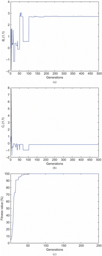
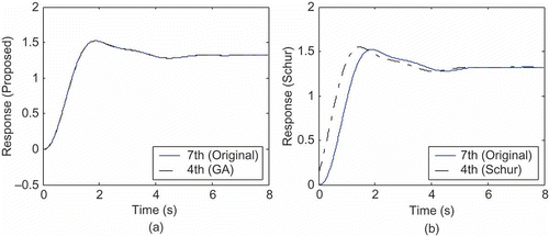
Figure 5. System output step responses corresponding to the reduced-order and the full-order models. (a) Proposed reduced-order model and (b) Schur reduced-order model.

4.1.2. MIMO model

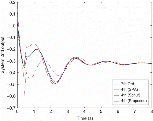
As a MIMO system, the original seventh-order MIMO system is now considered. The reduced-order models of the different methods are shown in Table 2 (except for the POD method that was reported for SISO only by the author [6]). As observed for retaining the dominant frequencies, the proposed method outperforms the others. The Schur method, however, gives similar results to our new method. Therefore, we further investigate the behaviour of these reduced models. For a step input, the first output response is shown in Figure 6. Notice that the Schur results are much far from being close to the original system response, whereas the others are closer. To evaluate the robustness of the proposed method in addition to retaining the dominant frequencies, the MIMO reduced-order models are simulated with a step input and different weights of state initial conditions. Results of simulations are shown in Figure 7 for the second system output. As observed, it can be clearly seen that the proposed GA reduction method provides the response that is the closest to the full-order model.

Table 2. MOR results comparison for MIMO systems

System	[Ar ]	[Br ]	[Cr ]	[Dr ]	λ
Original 7th order	Given	–	–	–	−0.5532 ± 8.1342i
					−0.8701 ± 1.3728i
					−03.0484
					−12.5882
					−13.2770
Proposed GA 4th order				[0]	−0.5532 ± 3.1342i
					−0.8701 ± 1.3728i
SPA 4th order					−0.5609 ± 3.1073i
					−0.8538 ± 4.3837i
Schur 4th order					−0.5532 ± 3.1342i
					−0.8701 ± 1.3728i

Figure 6. System first output step response of the full-order and reduced-order models.

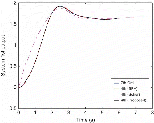
Figure 7. System second output response to step input along with initial conditions.

4.2. Example 2

In this example, we will investigate the new reduction technique by focusing on a system TF that has been recently considered by different researchers to retain its dominant frequencies [16,21–24 24]. It is to be noted that the presented methods are concerned with SISO-type systems with only real frequencies [36], whereas the new method deals with SISO- and/or MIMO-type systems with real and/or complex frequencies. However, we will use them to evaluate the performance of the new GA method. Now, the TF is given by

(19)

with λ = {−1, −2, −3, −4}. Using the GA reduction method, we will obtain a reduced-order model with frequencies that are exactly −1 and −2. Table 3 shows the proposed reduced-order model along with some others. Comparison of the results is performed based on retaining the dominant frequencies in the reduced-order model and on obtaining a response with minimum ISE given by

(20)

Table 3. Comparison of the reduced-order models, proposed and other methods

Reduction method	Transfer function	λ	ISE
Proposed GA reduced model		−1,−2	2.3785 × 10^−4
Parmar et al. reduced model [16]		−1,−4	2.64337 × 10^−4
Mittal et al. reduced model [21]		−1,−2	2.3785 × 10^−4
Mukherjee and Mishra reduced model [22]		−1,−2	2.37856 × 10^−4
Lucas reduced model [23]		−1,−2	3.58814 × 10^−4
Shamash reduced model [24]		−1,−2	3.3086 × 10^−4

As observed in Table 3, such results validate the performance of our proposed GA-MOR technique.

4.3. Example 3

In this final example, we will consider an eighth-order system TF that has been recently considered by different researchers [16,37–40 40]. However, we will now apply the proposed GA reduction method without the restriction of retaining the system dominant frequencies in the reduced-order model. The TF is given by

(21)

with λ = {−1, −2, −3, −4, −5, −6, −7, −8}. Using the proposed GA-MOR method, a second-order reduced model with λ = {−0.8669, −6.0327}) is obtained. Table 4 presents the GA second-order reduced model along with other reduced models of different reduction methods. In addition, step responses of the full-order and reduced-order models corresponding to the proposed and the recently published work of Parmar et al. [16] and Mukherjee et al. [37] are shown in Figure 8. The superiority of the new method can be clearly seen in Table 4 and Figure 8, where the ISE is much less and the response is much closer to the full-order model than all of the others.

Table 4. Comparison of reduced-order models

System	Reduced-order model	ISE
Proposed GA reduced model		7.4277 × 10^−4
Parmar et al. reduced model [16]		4.8090 × 10^−2
Mukherjee et al. reduced model [37]		5.6897 × 10^−2
Prasad and Pal reduced model [38]		1.4584
Gutman et al. reduced model [39]		1.3760
Chen et al. reduced model [40]		7.2101

Figure 8. System output step responses of the original and reduced-order models.

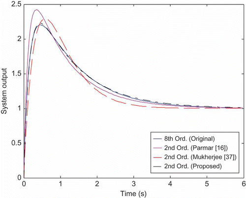
Based on the previous examples, as an off-line operation, the GA-MOR approach has shown to perform very effectively. This was proven, precisely, as seen in Example 3. Using the new approach, the ISE in Example 3 was found to be 7.4277 × 10 ⁻⁴ whereas the best value, using the other methods of recently published work, was only 5.6897 × 10⁻² or 4.8090 × 10 ⁻² [16,36], respectively. The improvement of the reduced-order model response using the proposed GA-MOR method may also be observed as seen in Figure 8.

5. Conclusion

A new method of GA with frequency selectivity for MOR of MIMO systems has been presented in this article. The new reduction method is achieved based on the implementation of GA-based evolutionary optimization technique. The reduced-order model is obtained based on the minimization of a mean square error criterion and maximization of the fitness function. Simulation results show the performance of the proposed GA-based method compared with other well-known methods in terms of maintaining system stability, preserving the exact dominant frequencies, providing system response for SISO- as well as MIMO-type systems with lowest ISE and providing system robustness performance corresponding to initial conditions. In addition, as a powerful nature of the proposed GA-MOR method, wherever there is an optimal solution, the GA will try to reach for it with accuracy depending on the designer constraints. Based on the results obtained by the illustrative examples, it is concluded that the proposed method outperforms the other methods in terms of robustness and objective achievement.

Acknowledgement

The authors sincerely thank the anonymous reviewers for their valuable comments, which indeed raised the level of the article presentation.

Appendix 1. Complex frequency

For a parallel source free RLC network [36], consider the non-zero initial condition differential equation given by

(22)

whose solution v(t) is desired. Being as general as possible, assume

(23)

allowing A and s to be complex numbers if necessary. Substituting Equation (23)(23) into Equation (22)(22) yields

(24)

or

(25)

One way to satisfy this equation is by equating the second term in Equation (25)(25) to zero:

(26)

where this equation is usually called the auxiliary equation or the characteristic equation. As Equation (26)(26) is a quadratic equation, there are two solutions, identified as s ₁ and s ₂:

(27)

(28)

Proper substitution and simplification leads to the following solution of v(t):

(29)

where A ₁ and A ₂ are selected to satisfy the initial conditions. s ₁ and s ₂ can be real or conjugate complex numbers, depending upon the values of R, L and C. In Equation (29)(29), as the exponents s ₁ t and s ₂ t must be dimensionless, s ₁ and s ₂ must have the unit of ‘per second’ (which is frequency). This means that s ₁ and s ₂ are in fact frequencies. Hence, in Equations (27)(27) and (28)(28), the exponential damping coefficient σ is called neper frequency. In the case where s ₁ and s ₂ are conjugate complex numbers, s ₁ and s ₂ are called complex frequencies [36].

References

- Phillips , J.R. 2000 . Model reduction of time-varying linear systems using approximate multipoint Krylov-subspace based reduced-order models . IEEE Trans. Circuits Sys. II , 47 : 239 – 248 .
- Phillips , J.R. Projection frameworks for model reduction of weakly nonlinear systems . 37th ACM/IEEE Design Automation Conference . Los Angeles, CA. June . pp. 184 – 189 .
- Kokotovic , P. , Khalil , H. and O'Reilly , J. 1986 . Singular Perturbation Methods in Control: Analysis and Design , Orlando, FL : Academic Press .
- Fridman , E. 2006 . Robust sampled-data H∞ control of linear singularly perturbed systems . IEEE Trans. Automat. Contr. , 51 : 470 – 475 .
- Benner , P. 2008 . Model reduction at ICIAM′07′, SIAM News , 40 : 1 – 3 .
- Bui-Thanh , T. and Willcox , K. Model reduction for large-scale CFD applications using the balanced proper orthogonal decomposition . 17th American Institute of Aeronautics and Astronautics Computational Fluid Dynamics Conference (AIAA 2005–4617) . Toronto, ON. June . pp. 1 – 12 .
- Stykel , T. 2006 . Balanced truncation model reduction for semidiscretized equation . Linear Algebra Appl. , 415 : 262 – 289 .
- Reis , T. and Stykel , T. 2008 . Balanced truncation model reduction of second-order systems . Math. Comput. Model. Dyn. Syst. , 14 : 391 – 406 .
- Datta , B.N. Finite element model updating and partial eigenvalue assignment in structural dynamics: Recent developments on computational methods . Proceedings of the 10th International Conference MMA2005&CMAM2 . Trakai. pp. 15 – 27 .
- Willcox , K. and Perarie , J. 2002 . Balanced model reduction via the proper orthogonal decomposition . AIAA. J. , 40 : 2323 – 2330 .
- Fujimoto , K. and Scherpen , J.M.A. Balancing and model reduction for discrete-time nonlinear systems based on Hankel singular value analysis . Proceedings of the MTNS . 2004 , Leuven, Belgium. July . pp. 343 – 347 .
- Heydari , P. and Pedram , M. 2006 . Model-order reduction using variational balanced truncation with spectral shaping . IEEE Trans. Circuits Syst. I , 53 : 879 – 891 .
- Rabiei , P. and Pedram , M. Model-order reduction of large circuits using balanced truncation . Proceedings of the IEEE ASP-DAC . Wanchai, Hong Kong. January . pp. 237 – 240 .
- Gugercin , S. , Athanasios , C. , Antoulas , A.C. and Beattie , C. A rational Krylov iteration for optimal H2 model reduction . Proceedings of the 17th International Symposium on Mathematical Theory on Networks and Systems . Kyoto, Japan. pp. 1665 – 1667 .
- Obinata , G. and Anderson , B.D.O. 2001 . Model Reduction for Control System Design , London : Springer-Verlag .
- Parmar , G. , Mukherjee , S. and Prasad , R. 2007 . System reduction using factor division algorithm and eigen spectrum analysis . Appl. Math. Model. , 31 : 2542 – 2552 .
- Panda , S. , Yadav , J.S. , Padidar , N.P. and Ardil , C. 2009 . Evolutionary techniques for model order reduction of large scale linear systems . Int. J. Appl. Sci. Eng. Technol. , 5 : 22 – 28 .
- Vishwakarma , C.B. and Prasad , R. 2009 . MIMO system reduction using modified pole clustering and genetic algorithm . Model. Simul. Eng. 2009 (ID 540895) , : 1 – 5 .
- Parmar , G. , Pandey , M.K. and Kumar , V. System order reduction using GA for unit impulse input and a comparative study using ISE & IRE . International Conference on Advances in Computing, Communication and Control . Mumbai, India. January . pp. 23 – 24 .
- Safonov , M.G. and Chiang , R.Y. 1989 . A Schur method for balanced-truncation model reduction . IEEE Trans. Automat. Contr. , 34 : 729 – 733 .
- Mittal , A.K. , Prasad , P. and Sharma , S.P. 2004 . Reduction of linear dynamic systems using an error minimization technique . J. Inst. Eng. IE (I) J. EL , 84 : 201 – 206 .
- Mukherjee , S. and Mishra , R.N. 1987 . Order reduction of linear systems using an error minimization technique . J. Franklin Inst. , 323 : 23 – 32 .
- Lucas , T.N. 1983 . Factor division: A useful algorithm in model reduction . IEE Proc. , 130 : 362 – 364 .
- Shamash , Y. 1975 . Linear system reduction using Pade approximation to allow retention of dominant modes . Int. J. Control , 21 : 257 – 272 .
- Varga , A. and Anderson , B.D.O. 2003 . Accuracy enhancing methods for balancing-related frequency-weighted model and controller reduction . Automatica , 39 : 919 – 927 .
- De Lathauwer , L. , De Moor , B. and Vandewalle , J. 2004 . Computation of the canonical decomposition by means of a simultaneous generalized Schur decomposition . SIAM J. Matrix Anal. Appl. , 26 : 295 – 327 .
- Stegeman , A. 2009 . Using the simultaneous generalized Schur decomposition as a Candecomp/Parafac algorithm for ill-conditioned data . J. Chemom. , 23 : 385 – 392 .
- Antoulas , A.C. 2005 . Approximation of Large-Scale Dynamical Systems, Advances in Design and Control , Philadelphia, PA : SIAM .
- Pereyra , V. and Kaelin , B. 2008 . Fast wave propagation by model order reduction . Electronic Trans. Numer. Anal. , 30 : 406 – 419 .
- Goldberg , D. 1989 . Genetic Algorithms in Search, Optimization, and Machine Learning , Upper Saddle River, NJ : Addison-Wesley Professional .
- Abo-Hammour , Z. , Mirza , N. , Mirza , S.M. and Arif , M. 2002 . Cartesian path generation of robot manipulators using continuous genetic algorithms . Rob. Auton. Syst. , 41 : 179 – 223 .
- Michalewics , Z. 1996 . Genetic Algorithms + Data Structure = Evolution Programs , 3rd , Berlin, New York, , Heidelberg : Springer-Verlag .
- Chang , W.D. 2006 . Coefficient estimation of IIR filter by a multiple crossover genetic algorithm . Comput. Math. Appl. , 51 : 1437 – 1444 .
- Iracleous , D. and Alexandridis , A. 1990 . A simple solution to the optimal eigenvalue assignment problem . IEEE Trans. Automat. Contr. , 9 : 1746 – 1749 .
- Mahalanabis , A. , Kothari , D. and Ahson , S. 1988 . Computer Aided Power Systems Analysis and Control , New Delhi : McGraw-Hill .
- Hayt , W.H. , Kemmerly , J.E. and Durbin , S.M. 2007 . Engineering Circuit Analysis , 322 New York : McGraw-Hill .
- Mukherjee , S. , Satakshi , M. and Mittal , R.C. 2005 . Model order reduction using response matching technique . J. Franklin Inst. , 342 : 503 – 519 .
- Prasad , R. and Pal , J. 1991 . Stable reduction of linear systems by continued fractions . J. Inst. Eng. IE (I) J. EL , 72 : 113 – 116 .
- Gutman , P. , Mannerfelt , C.F. and Molander , P. 1982 . Contributions to the model reduction problem . IEEE Trans. Automat. Contr. AC- , 27 : 454 – 455 .
- Chen , T.C. , Chang , C.Y. and Han , K.W. 1980 . Model reduction using the stability equation method and the continued fraction method . Int. J. Control , 32 : 81 – 94 .