Comparison of the reduced-basis and POD a posteriori error estimators for an elliptic linear-quadratic optimal control problem

Abstract

In this article, a linear-quadratic optimal control problem governed by the Helmholtz equation is considered. For the computation of suboptimal solutions, two different model reduction techniques are compared: the reduced-basis method and proper orthogonal decomposition. By an a posteriori error estimator for the optimal control problem, the accuracy of the suboptimal solutions is ensured. The efficiency of both model reduction approaches is illustrated by a numerical example for the stationary Helmholtz equation.

Keywords:

• optimal control
• a posteriori error estimate
• proper orthogonal decomposition
• reduced-basis method
• Helmholtz equation

1. Introduction

Optimal control problems for partial differential equations are often hard to tackle numerically because their discretization leads to very large-scale optimization problems. Therefore, different techniques of model reduction have been developed to approximate these problems by smaller ones that are tractable with less effort. Among them, the reduced-basis method (RBM) [Meiner Meinung nach sollten wir noch RB durch RBM ersetzen, vgl. abstract] and the proper orthogonal decomposition (POD) are widely used also in the context of non-linear problems.

Some reduced-order methods such as balanced truncation offer a reliable a priori error analysis for optimal control applications [1,2], however, on a discrete level. On the contrary, for POD and RBM it is not a priori clear how far the optimal control of the reduced-order problem is from the exact one, unless its snapshots are generating a sufficiently rich space, where sufficiently rich implies that the space contains all possible snapshots. However, we are able to compensate for the lack of a priori analysis for POD and RBM by utilizing an a posteriori analysis. This approach is based on a fairly standard perturbation argument to deduce how far the suboptimal control, computed on the basis of the reduced-order method, is away from the (unknown) exact one.

Finally, we mention that in [3] the application of RBM for parametrized optimal control problems has been considered too.

2. The optimal control problem and optimality conditions

In this section, we introduce the linear-quadratic elliptic optimal control problem, recall the associated first-order necessary optimality conditions and define a reduced problem only for the control variable.

2.1. The optimal control problem

Suppose that the interior of a car is simplified by the two-dimensional domain plotted in Figure 1(a) [Noch in s/w]. The boundary is split into two measurable disjunct parts and .

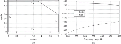
Figure 1. (a) Two-dimensional cross section of an idealized interior of the vehicle and boundary parts and ; (b) impedance values for melamine 50 mm width in the frequency range from 200 to 500 Hz.

Denoting the frequency by f, let (see Figure 1(b)) be a given complex impedance. Then, the associated sound pressure is governed by the Helmholtz equation

1a

together with the boundary conditions

1b

1c

In Equation (1)1a, is an ambient density, is the angular frequency and is the wave number, where the constant denotes the speed of sound. The right-hand side is a simplified model for a source at the point (e.g. a loudspeaker located at ) with the intensity , , and shape function

For the normal impedance boundary condition (1b), let be the imaginary unit and denote the derivative in the outward normal direction. All other parts on the boundary are assumed to be perfectly rigid, see Equation (1c)1c.

In [4] the impedance is identified by using techniques from infinite-dimensional optimization. We refer to [5], where an optimal control problem for an impedance factor is studied. The frequency is kept fixed and the goal is to obtain the least amount of noise propagation to the far field. Let us also cite [6], where the authors deal with the Helmholtz equation with Dirac delta measures as inhomogeneity.

Throughout this article, we suppose the following assumption.

Assumption 2.1:

For all given frequencies , all given and the impedance function , plotted in Figure 1(b) , the problem (1) admits a unique solution .

Remark 2.1:

Due to the Fredholm theory, [7], we can ensure existence of a unique solution provided is not an eigenvalue of considered on with Neumann and Robin boundary conditions on and , respectively.

Let , , , be measured sound pressures at different given observation points , , for a given frequency , see Figure 2. We introduce the quadratic cost functional

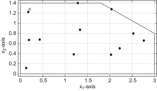
Figure 2. Measurement points (•) and location of the source () for our numerical examples.

where is a given reference intensity, is the absolute modulus of a complex number z, is non-negative and is positive. Then, given f, we consider the optimal control problem

Thus, (P _f ) is a linear-quadratic optimal control problem for any frequency .

2.2. First-order optimality conditions

The first-order necessary optimality conditions to consist of the state equation, the adjoint system for the Lagrange multiplier

and the equation for the optimal control

where denotes the Dirac delta distribution satisfying

As usual is the complex conjugate of . For more details, we refer the reader to [4,8].

2.3. The reduced problem

Motivated by Assumption 2.1, we introduce the reduced cost functional by

where again denotes the unique solution to Equation (1)1a for a given control input u at a given frequency f. Then, is equivalent to the reduced optimal control problem

If is an optimal solution to , then solves . On the other hand, if is an optimal solution to (), then the pair solves (). The ultimate goal is to determine the optimal control for many values . To avoid a naive and possibly costly evaluation of the elliptic linear-quadratic optimal control problem for various values of f, we introduce a model reduction. This leads to a reduced-order model for . The accuracy of the reduced-order model is controlled by an a posteriori error analysis. This is the focus of the next section.

3. A posteriori error estimate for the optimal control problem

In this section, we recall some results of the a posteriori error estimator. For more details, we refer the reader to [9,10]. Suppose that is an arbitrary control input. Then, the difference can be estimated without requiring knowledge of .

Theorem 3.1:

Let be an optimal solution to (). Let and be the associated state variable and Lagrange multiplier, respectively. Suppose that is chosen arbitrarily, solves Equation (1)1a and solves

2

Then, it follows that

3

where .

Proof:

The claim follows from Theorem 3.1, Proposition 3.2 and Remark 3.3 in [9].

We will call the right-hand side of Equation (3)3 an a posteriori error estimate because in the next two sections, we shall apply it to suboptimal controls that have been computed from a reduced-order model. After having computed , we determine the associated state and adjoint state . Then, we can compute and its norm s.t. Equation (3)3 gives an upper bound for the distance of to . In this way, the error caused by the reduced-order model can be estimated a posteriori. If the error is too large, we have to include more basis functions into the reduced model.

4. Reduced-order methods

In this section, we introduce the reduced-order modelling for Equation (1)1a utilizing the POD and the RBM. Let us emphasize that the computation of the reduced-order model is only based on the state Equation (1)1a, so that no information from the optimal solution of is needed.

For solving the state Equation (1)1a numerically, we introduce a finite-dimensional subspace X of the Sobolev space , where for our application X is a finite element (FE) space of dimension . Moreover, for the inner product in X, that is for , we consider both the -inner product as well as the -inner product

For modelling complex-valued functions, we continue by introducing the tensor product Hilbert space endowed with the inner product where and . Then from Equation (1)1a the following linear system of equations arises: for given frequency and given control find , s.t.

4

where , and

5a

5b

Note, that for any we use the notations and . Moreover, in Equation (5)5a and the definition of , , we abbreviate , and , each for .

Next, for any frequency and any control it is readily seen that if is a solution of Equation (4)4, then is a discrete approximation (consisting of degrees of freedom) of the weak solution of Equation (1)1a. Obviously, in view of Assumption 2.1, we have to assume that Equation (4)4 possesses a unique solution for all frequencies , too, which can be assured either by a Fredholm-type argument in analogy to Remark 2.1 or by the positivity of the inf–sup stability factor, that is,

6

Finally, we consider subspaces and , where and are spanned by (global) basis functions and , . Applying the Galerkin projection of Equation (4)4 onto yields the reduced-order model: find , s.t.

7

As all bilinear forms in the definitions of and , that is, s, m and q, are independent of the frequency f and the control u, respectively, solving Equation (7)7 can be decoupled into an offline/online phase, once the basis functions and , , are known. Performing this decoupling results in an online complexity of for assembling Equation (7)7 and an additional for solving. Hence, the coefficients of the reduced-order solution can be obtained rapidly, that is, with complexity independent of . For more details on this offline/online decoupling, we refer to [11].

At this point we note that the POD and the RBM mainly differ in the way the basis functions and , , are generated, which is reviewed for both in the sequel. However, before doing so we finally note that if solves Equation (4)4 and if solves Equation (7)7, both for fixed frequency and for fixed control , then from Equation (6)6 we infer that

8

Hence, is an a posteriori error estimator for , which is only needed in the RBM subsection, but obviously also holds true for the POD.

4.1. Proper orthogonal decomposition

In this subsection, we briefly review the POD method to derive the basis functions and , , for the reduced-order model Equation (7)7. Note that Equation (4)4 is a linear elliptic equation and u is a complex number. Thus, by linear superposition for any frequency f, the solution to Equation (4)4 satisfies .

Let be a given snapshot grid. We consider the corresponding snapshot space with , where we abbreviate and , . Then, for given , the POD basis functions , , of are determined from the minimization problem

9

Remark 4.1:

In some applications, the mean value of the snapshots is included in the POD modelling (see, e.g. in [12]). In our numerical experiments, it turns out that this approach does not give rise to better results.

The solution to Equation (9)9 is given by the solution of the eigenvalue problem

where is a linear, bounded, compact, self-adjoint and non-negative operator; see [12]. Thus, there exists an orthonormal set of eigenfunctions and corresponding non-negative eigenvalues satisfying

In [13] the dependence of and for on the chosen snapshot grid is investigated.

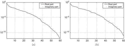
Analogously, a POD basis for the snapshot space can be introduced. As the eigenvalues for the real and for the imaginary parts decay in a similar rate (see Figure 3), we choose the same number of ansatz functions for the real and for the imaginary parts, which justifies the definition of by for Equation (7)7. To highlight similarities and differences of the POD and the RBM, we stress that the modes are linear combinations of all snapshots , .

Figure 3. Decay of the first 60 POD eigenvalues for (a) and (b) .

4.2. The reduced-basis method

Recall that denotes the frequency snapshot grid, which we now extend by the control, that is, we introduce and . Then, for the POD, the snapshots are the solutions of Equation (4)4 for all . In contrast to this, for the RBM, the Helmholtz equation (4)4 has to be solved for some particular values in , only, where the selection procedure is given below.

We start by introducing some notation. Let , , denote the set of identified parameters. Then, the (hierarchical) RBM approximation spaces are given by and . Note that for algebraic stability of the reduced-order model (7), the basis functions and are orthonormalized w.r.t. by a Gram–Schmidt procedure (see [11]). Hence, the modes are linear combinations of just a few snapshots only.

Table

Algorithm 4.1:
1: Set , and choose arbitrarily.
2: for to do
3:Compute .
4:if or then
5:break.
6:else
7:Set
8:Compute .
9:Set and .
10:end if
11:end for

To identify frequencies in , which lead to ‘good’ approximation spaces and , we utilize the standard greedy procedure (see [11]), which reads as follows:

Note that in Algorithm 4.1 denotes the a posteriori error estimator introduced in Equation (8)8. Recall that this error estimator consists of two computational parts, namely the inverse of the inf–sup stability factor and the dual norms (w.r.t. X) of , . Obviously, for the efficiency of Algorithm 4.1 both parts have to be rapidly evaluable. Whereas similar to the solution of the reduced-order model (7), the computation of the latter can be decoupled into offline/online phase (see [11]), resulting in an online complexity of , the computation of is even more involved than solving the actual problem (4). Hence, has to be replaced by a rapidly evaluable approximation , s.t. by we denote the approximation of resulting from substituting by in Equation (8)8.

In the RBM context, usually is a lower bound to , s.t. remains a rigorous a posteriori error estimator. This lower bound can be obtained amongst others by the application of the so-called Successive Constraint Method (SCM, see [14]), which in fact provides both a lower bound and an upper bound to , that is, . The computation is once again decoupled into an offline/online phase, s.t. in the online phase can be determined by solving a (small) linear optimization problem in design variables. Moreover, the online complexity for computing the upper bound is , where K is a small number of (in the offline phase of the SCM by another greedy algorithm) identified frequencies . Hence, both bounds can be evaluated with a complexity that is independent of . For more details we refer to [14], and note that in this work a Helmholtz problem is also considered for the numerical experiments.

Unfortunately, the offline stage of the SCM, that is, basically the identification of , is quite extensive. However, in this work, we are interested in , the suboptimal solution to (), for which we already have a rigorous a posteriori error estimator (see Theorem 3.1). Hence, does not necessarily need to be rigorous, rather than a good indicator and the easiest way to avoid the cost of an extensive precomputation is to simply use . Another possibility is to skip the identification of in the SCM offline phase and just define , for (say) , and use , that is, the upper bound provided by the SCM. 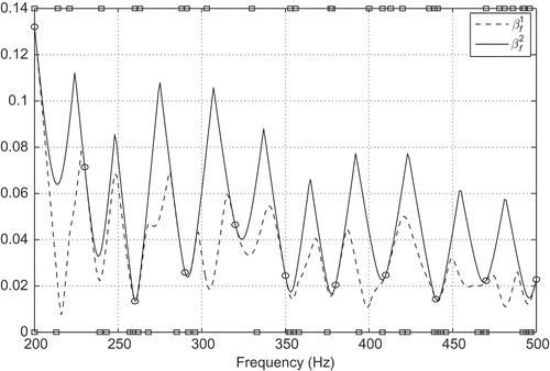Note that proceeding this way, we have to compute for all frequencies in , that is, we have to solve K eigenvalue problems. The CPU time is reported in Table 1. Moreover, Figure 4 visualizes as well as . The same figure also shows the values , identified by Algorithm 4.1, where is marked on the bottom (top) axis if (). We will investigate the differences resulting from using and as approximations to in Section 5.

Table 1. Run 1: CPU times in seconds

Snapshot generation with FE	50.9
POD computation	2.4
POD optimization for ,	181.4
POD optimization for ,	214.4
POD optimization for ,	293.6
POD optimization for ,	302.8
Approximation of inf–sup constant	0.0	84.9
RBM computation	38.0	38.1
RBM optimization for ,	169.9	154.7
RBM optimization for ,	160.8	167.5
RBM optimization for ,	291.0	280.7
RBM optimization for ,	282.2	270.2

Figure 4. Inf–sup constant , its approximation as well as identified by Algorithm 4.1.

Remark 4.2:

Note that for the POD method the bases and are computed, s.t. the mean error to the snapshots is minimized (see Equation (9)9), whereas for the RBM and are computed, s.t. the maximum error to the snapshots is minimized (see Algorithm 4.1). A detailed comparison of the POD and the RBM has been carried out in [11] for a steady conduction problem. Moreover, in the context of instationary parametrized PDEs both methods are merged, s.t. in the greedy procedure (performed in the offline phase) the next parameter is identified as in Algorithm 4.1, but the basis functions themselves are obtained by performing a POD (in time) for this identified parameter (see [15,16]).

4.3. The a posteriori error estimator for ()

The a posteriori error estimator for () is formulated in Algorithm 4.2.

Table

Algorithm 4.2:
1: Choose , , and . Set .
2: for to 500 do
3:
4:repeat
5:Set .
6:Calculate the suboptimal solution to
7:Compute the solutions to (1) for and to (4) for .
8:Set .
9:if then
10:Set .
11:Return , , and STOP.
12:else
13:Set .
14:end if
15:until
16:if then
17:Increase and restart the algorithm.
18:break.
19:end if
20:end for

5. Numerical experiments

In this section, we present numerical experiments. One example is constructed in such a way that the optimal control is known. Thus, we can verify the quality of the estimate (3). In the second example, the (exact) optimal control is unknown. All coding is done in Matlab using routines from the PDE Toolbox with FE. We apply a standard piecewise linear FE discretization with degrees of freedom.

Run 1:

Let the impedance be given for the material melamine with depth; see Figure 1. We choose for the cost functional , and

The measurement points , with are depicted in Figure 2. The values , , are given by , that is, by the solution to Equation (1)1a evaluated at for and . Then, the optimal solution to () is for . First, we apply Algorithm 4.2 for the tolerance . In Figure 5, we present the number of of utilized POD basis functions for the choices and . It turns out that the required tolerance is achieved for all with basis functions. We observe that the number of POD basis functions changes over the frequency band . Moreover, the different choices for X also influences the value of . The results for the RBM are given in Figure 6.

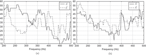
Figure 5. Run 1: Number of POD ansatz functions over the frequency band (a) for and (b) for with the tolerance for the a posteriori error estimator.

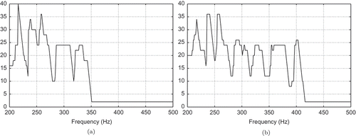
Figure 6. Run 1: Number of RB ansatz functions over the frequency band (a) for and (b) for with the tolerance for the a posteriori error estimator.

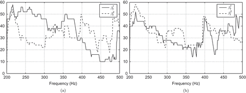
Compared with the POD approximations, the RBM needs more basis functions at the beginning, but (significantly) less for . The needed CPU times are presented in Table 1. Note that for RBM Table 1 contains two columns, where the first one corresponds to and the second one to for approximating .

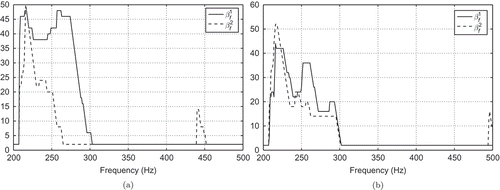
Next, we apply Algorithm 4.2 again with the smaller tolerance . In Figure 7, the number of utilized POD basis functions is plotted. The results for the RBM are given in Figure 8. Again, the required tolerance is achieved for all variants of the POD and the RBM. As expected, more basis functions have to be included in our reduced-order modelling. Recall that denotes the optimal solution to () and denotes the suboptimal solution obtained from using basis functions. The decay of is visualized in Figure 9 for using the POD and the RBM. Note that we do not present the effectivity, that is, the ratio between the true error and its estimator , as it turns out to be bounded by 1.1 for all .

Figure 9. Run 1: Decay of for POD and RBM in .

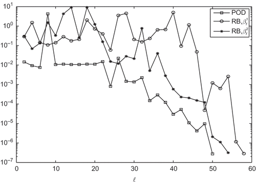
Figure 7. Run 1: Number of POD ansatz functions over the frequency band (a) for and (b) for with the tolerance for the a posteriori error estimator.

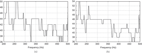
Figure 8. Run 1: Number of RB ansatz functions over the frequency band (a) for and (b) for with the tolerance for the a posteriori error estimator.

Run 2:

In the second example, we choose the same parameter as in the first run, but now . Thus, the optimal solution to is not known. We apply Algorithm 4.2 with the tolerance . In Figure 10, the number of utilized POD basis functions is plotted. The results for the RBM are given in Figure 11.

Figure 10. Run 2: Number of POD ansatz functions over the frequency band (a) for and (b) for with the tolerance for the a posteriori error estimator.

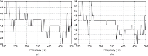
Figure 11. Run 2: Number of RB ansatz functions over the frequency band (a) for and (b) for with the tolerance for the a posteriori error estimator.

6. Conclusion

We have compared RBM and POD for a linear-quadratic optimal control problem that which is constrained by the Helmholtz equation. Thus, the following conclusions hold for this particular problem only. Moreover, it should be noted that the control (and thus the parameters for RBM and POD) is only formally two dimensional (real and imaginary parts), since we have seen that linear superposition allows to reduce the parameter dimension.

We have demonstrated that both methods are quite efficient, the differences are more or less marginal. As we can see in Table 1, RBM is a little more efficient than POD as long as we can avoid the computation of an approximation for the inf–sup constant. Also the average number of RBM modes is smaller than than the one for POD as we can deduce by the comparison of Figures 5 and 6 and Figures 7 and 8 for Run 1, Figures 10 and 11 for Run 2 as well as the CPU timings for Algorithm 4.3 in Table 1. On the other hand, Figure 9 shows that the true error in over the frequency sample is smaller for POD. This is somehow astonishing, because the POD is known to be the best approximation of the state whereas here we consider the control as the best approximation. It also seems that POD reaches the asymptotic regime earlier.

Acknowledgements

The author T.T. has been supported by the state of Baden-Württemberg within the Landesgraduierten-Programm. The author S.V. gratefully acknowledges the support given by the Austrian Science Fund under grant no. P19588-N18.

References

- Antoulas , A.C. 2005 . Approximation of Large-Scale Dynamical Systems (Advances in Design and Control) , Philadelphia, PA : Society for Industrial and Applied Mathematics .
- Benner , P. and Quintana-Ortí , E.S. 2005 . “ Model reduction based on spectral projection methods ” . In Dimension Reduction of Large-Scale Systems , Edited by: Benner , P. , Mehrmann , V. and Sorensen , D.C. 5 – 45 . Berlin : Springer-Verlag .
- Quarteroni , A. , Rozza , G. , Dedè , L. and Quaini , A. 2006 . “ Numerical approximation of a control problem for advection-diffusion processes ” . In IFIP International Federation for Information Processing , Vol. 199 , 261 – 273 . Boston, MA : Springer .
- Volkwein , S. and Hepberger , A. 2008 . Impedance identification by POD model reduction techniques . Automatisierungstechnik , 8 : 437 – 446 .
- Cao , M.H.Y. and Yang , H. 2007 . Estimation of optimal acoustic linear impedance factor for reduction of radiated noise . Int. J. Numer. Anal. Model. , 4 : 116 – 126 .
- Bermúdez , P.G.A. and Rodríguez , R. 2004 . Finite element methods in local active control of sound . SIAM J. Control Optim. , 4 : 437 – 465 .
- Reed , S. and Simon , B. 1980 . Methods of Modern Mathematical Physics, I. Functional Analysis , 2nd , San Diego, CA : Academic Press .
- Volkwein , S. 2010 . Admittance identification from point-wise sound pressure measurements using reduced-order modelling . J. Optim. Theory Appl. , 147 : 169 – 193 .
- Tröltzsch , F. and Volkwein , S. 2009 . POD a posteriori error estimates for linear-quadratic optimal control problems . Comput. Optim. Appl. , 44 : 83 – 115 .
- Kahlbacher , M. and Volkwein , S. submitted 2010 . POD a posteriori error based inexact SQP method for bilinear elliptic optimal control problems ,
- Rozza , G. , Huynh , D. and Patera , A. 2007 . Reduced basis approximation and a posteriori error estimation for affinely parametrized elliptic coercive partial differential equations . Arch. Comput. Method. Eng. , 15 : 229 – 275 .
- Holmes , P. , Lumley , J. and Berkooz , G. 1996 . Turbulence, Coherent Structures, Dynamical Systems and Symmetry , Cambridge : Cambridge University Press .
- Kunisch , K. and Volkwein , S. 2002 . Galerkin proper orthogonal decomposition methods for a general equation in fluid dynamics . SIAM J. Numer. Anal. , 40 : 492 – 515 .
- Huynh , D. , Rozza , G. , Sen , S. and Patera , A. 2007 . A successive constraint linear optimization method for lower bounds of parametric coercivity and inf–sup stability constants . C. R. Math. , 345 : 473 – 478 .
- Haasdonk , B. and Ohlberger , M. 2008 . Reduced basis method for finite volume approximations of parametrized linear evolution equations . ESAIM: M2AN , 42 : 277 – 302 .
- Nguyen , N.C. , Rozza , G. and Patera , A. 2009 . Reduced basis approximation and a posteriori error estimation for the time-dependent viscous Burgers equation . Calcolo , 46 : 157 – 185 .