Passivity preserving parametric model-order reduction for non-affine parameters

Abstract

Parametric model-order reduction (pMOR) has become a well-established technology for analysing large-scale systems with multiple parameters. However, the treatment of non-affine parameters is still posing significant challenges, because projection-based order-reduction methods cannot be applied directly. A common remedy is to establish affine parameter-dependencies approximately, but present extraction methods do not take important system properties, such as passivity, into account. This article proposes a new order-reduction approach that preserves passivity, reciprocity and causality and applies to a wide class of linear time-invariant (LTI) systems. We present the theory of the suggested method and demonstrate its practical usefulness by numerical examples taken from computational electromagnetics.

Keywords:

• model-order reduction
• multi-parameter system
• non-affine parameters
• passivity

1. Introduction

Parametric model-order reduction (pMOR) denotes a family of powerful technologies for reducing the numerical costs for solving systems with multiple parameters. There are two major classes of pMOR methods: the first one constructs a parametric reduced-order model (ROM) by interpolating either the system matrices [1,2] or the transfer function [3] of local non-parametric ROMs. The second class, which this article focuses on, is based on the application of global projection matrices onto a parameterized original model. These methods can be further categorized as single-point [4–9] or multi-point [10,11] methods, respectively, and they all require affine parameterization, that is, the parameters must appear explicitly in the governing equations. Today's single-point methods are restricted to multi-linear [5,7,8] or polynomial [4,12] parameter-dependence.

Perhaps the most common case of affine parameter-dependence is that of the operating frequency in linear time-invariant (LTI) systems. An important example of non-affine parameterization is given by geometric design variables in the finite-element (FE) method.

In this article, we consider a class of LTI systems that is characterized by very large-scale affine frequency-dependence and the presence of additional non-affine parameters. Such systems arise in, for example, circuit simulation [13], dynamical analysis of mechanical structures [14] and FE simulation of electromagnetic fields [15]. To make them accessible to the pMOR methods above, some pre-processing is necessary to establish affine parameterization. As existing methods [16,17] are highly specialized and require major modifications to the underlying simulation software, we have suggested in [18] a simple and rather generic alternative; to instantiate the original system at discrete points in parameter space and apply polynomial interpolation to the system matrices. The interpolated system thus obtained is suitable for projection-based pMOR but, as we shall prove in this article, the resulting ROM may not preserve the passivity of the original system and thus violate a crucial prerequisite for subsequent system level simulations. Based on our analysis, we shall develop an improved pMOR method that is guaranteed to preserve passivity, reciprocity and causality. Its key components are given by a modified interpolation scheme and an augmented projection matrix.

The remainder of this article is organized as follows: Section 2 describes an abstract prototype system and gives a proof of passivity. Section 3 presents our basic pMOR methodology for non-affine parameters and analyses the failure mechanisms associated with its naive implementation. Section 4 describes an enhanced pMOR method that is proven to preserve important system properties, and is the main contribution of this article. Section 6 presents numerical exampled to demonstrate the reliability and practical usefulness of the suggested approach. This article concludes with a short summary and outlook to future research.

2. Original model

We consider parameterized systems of the form

(1a)

(1b)

where , , , and . The complex frequency is denoted by , and represents the parameter vector. The abbreviations and stand for transpose and conjugate transpose, respectively. We assume that is symmetric positive definite (spd) and that the matrices and are symmetric positive semi-definite (spsd) and possess partitionings of the form

(2)

where , is spd and is a properly chosen permutation matrix. The transfer function of the system (1)(1b) is given by

(3)

Systems of this type arise in dynamic analysis of mechanical structures [14], circuit simulation of electrical networks consisting of Resistors, Inductors and Capacitors (RLC networks) [13] and computational electromagnetics [15].

Also, note that the system (1) may not be well defined in the case , because the matrix is only required to be spsd. This behaviour is typical for nodal analysis in circuit simulation [19] and field formulations in electromagnetics [20].

The fact that the output matrix is assumed to be of the form , that is, the transpose of the input matrix , together with the symmetry of the matrices , implies that the transfer matrix is symmetric. Such symmetry is characteristic for a wide class of systems: in particular, when describes an impedance or admittance matrix, the system is reciprocal [21].

2.1. Passivity of original system

We start with a fundamental theorem from [22]:

Theorem 2.1: The transfer function of a system in impedance or admittance form represents a passive linear system if and only if

(C1) All elements of are analytic for .

(C2) for all .

(C3) .

Lemma 2.2: System (1) is passive.

Proof: The proof is by verifying properties (C1)–(C3) of Theorem 2.1. To simplify notation, we omit the explicit dependence of the system-matrices.

(C1) As , are spsd and is spd, all poles of

(4)

lie in the closed left half-plane [14]. Multiplying Equation (4)(4) by B ^T from the left and by B from the right does not introduce any poles in the open right half-plane.

(C2) We now have to show that

(5)

Using Equation (3)(3), we obtain

(6)

By introducing the shorthand notation

(7)

and splitting into its real and imaginary parts, , Equation (6)(6) becomes

(8)

By assumption, and . Therefore .

(C3) With and real-valued, we have

(9)

3. Basic methodology of model-order reduction for non-affine parameters

A general prerequisite for pMOR methods is affine [10] parameter-dependence. This means that the system matrices and the right-hand side (r.h.s.) in Equation (1a) must be of the form

(10)

(11)

where are continuous functions of the parameters, and and denote the cardinalities of the sets and , respectively. Note that the system-matrix and the r.h.s. of Equation (1)(1b) exhibit affine parameterization in the complex frequency only. In the following, we shall first present a simple yet versatile method for establishing affine dependence on the other parameters, then give a generic description of the subsequent pMOR step and, finally, show that a naive implementation of such methodology will not preserve passivity of the system.

3.1. Extraction of affine parameters

A number of methods for extracting affine parameterization are already known from the literature [11,16,17,23–25]. However, they either do not lead to polynomial parameter-dependence globally or make pre-assumptions about the physical nature of the mathematical modelling technique for the system under consideration. Moreover, their computer implementation may require significant modifications of the computer software that sets up the system, for example, a circuit simulator or FE kernel.

The method we describe in the following [18] is very generic and aims at overcoming the limitations above for a broad class of applications. Neither does it require information about the physical nature of the system nor modifications to other software components. The sole pre-assumption is that all parameter-dependencies are continuous to allow for approximation by low-order polynomials.

We propose to replace the original system-matrices and r.h.s. by multivariate polynomial interpolations of low order, and . Hence we have

(12a)

(12b)

wherein and are coefficient matrices to be determined, and denotes a set of multivariate polynomials of interpolating type [26], satisfying the interpolation condition

(13)

at pairwise distinct interpolation points . By plugging Equation (13)(13) into Equation (12)(12b), the coefficient matrices and are seen to be uniquely defined by

(14a)

(14b)

provided that the set is unisolvent. Thus, by instantiating the system at the interpolation points, we obtain an approximate system :

(15a)

(15b)

that features affine, even polynomial, parameterization and is hence accessible to projection-based pMOR.

Note that the error in Equation (12)(12b) depends not only on the order of the polynomials but also on the choice of interpolation points. Motivated by [26] and the comparative study of [18], we prefer tensor grids based on the zeros of Tchebychev polynomials. Adaptive point-selection strategies are beyond the scope of this article.

3.2. Projection-based MOR

By restricting to the column space of a trial matrix , we obtain

(16)

and, by applying Petrov–Galerkin testing by a matrix to Equation (15a), we arrive at a ROM of the form

(17a)

(17b)

where

(18a)

(18b)

(18c)

As Equations (15)(15b) and (17), respectively, exhibit polynomial parameterization, both single-point [12] and multi-point methods [10,11] may be used to construct the projection matrices and .

3.3. Failure of passivity preservation

In Section 2.1, we proved the original system to be passive. We now investigate whether the family of MOR methods presented in Section 3 is able to preserve this property. As the projection step of Section 3.2 leaves the overall structure of the parameterization unchanged, we only need to examine what conditions the reduced system matrices , , , and have to fulfil to preserve passivity. As detailed in the proof of Lemma 2.2, the passivity of system (2) rests on two main properties:

• (P1) Hermitian positive semi-definiteness of and as well as Hermitian positive definiteness of . These matrix properties are required for Lemma 2.2, conditions (C1) and (C2).

• (P2) Realness of , , and . This is necessary to fulfil Lemma 2.2, condition (C3).

As the interpolation polynomials do not in general remain positive everywhere between the interpolation points, the interpolation strategy (12a) is not guaranteed to preserve positive (semi-)definiteness. We shall present numerical evidence for this deficiency in Section 6. Hence passivity may already get lost in the interpolated system (15), before the order-reduction step, so that the resulting ROM cannot be expected to possess property (P1).

For , the generalized state vectors x and are complex-valued. As the projection matrices generated by a single- or multi-point method are based on (moments of) x, they will, in general, be complex-valued, too. Hence property (P2) cannot be guaranteed.

Note that the breakdown of property (P1) is a consequence of the interpolation strategy, whereas that of property (P2) is inherent to the projection step in Equation (18)(18c). We conclude that the ROM does not inherit passivity from the original model.

4. Passivity preserving order-reduction method

We have shown above that the breakdown of property (P1) is a consequence of the interpolation strategy. To overcome this deficiency, we propose to interpolate not the matrices themselves, but rather their Cholesky factorizations , with . In case of the matrices and , which are only spsd, we take the Cholesky factors of the corresponding spd submatrices , introduced in Equation (2)(2). Based on the factorizations at the interpolation points ,

(19)

the interpolations of the Cholesky factors and system-matrices read

(20)

(21)

By construction, and are spsd. Similarly, is spd except on at most a set of measure zero of pathological points where may become spsd. To understand this restriction, consider as a special case of Equation (21)(21) the interpolation of a spd matrix of dimension 1, that is, a positive function of a single parameter . According to Equation (19)(19), the interpolated factorization reads

(22)

As may assume both signs, the polynomial on the r.h.s. may possess real-valued zeros . In consequence, we have for the interpolated function

(23)

even though . As the set of zeros of is given by the set of zeros of a polynomial, it is of measure zero.

Now that symmetric positive (semi-)definiteness of the interpolated matrices has been established almost everywhere, we have to make sure that this property is preserved by the projection step. This is achieved by choosing

(24)

Moreover, to re-establish property (P2), has to be real-valued.

At the same time, we wish to maintain the projection space of a proven MOR method, to preserve the quality of the ROM. The problem is that the trial matrices constructed by such methods, now denoted by , may become complex-valued, as discussed in Section 3.3. To resolve this conflict, we propose the following two-step approach:

1.	Take any suitable single- or multi-point pMOR method to compute a complex-valued trial matrix for an interpolated system based on Equation (21)(21).
2.	Construct the final, real-valued matrix from the real and imaginary parts of , such that

(25)

The procedure ensures both and , for the price of doubling the dimension of the ROM. The final ROM, hence, reads

(26a)

(26b)

with

(26c)

(26d)

The following theorem summarizes the system properties of the ROM.

Theorem 4.1: The reduced-order system (26) is passive, causal and reciprocal.

Proof: The ROM (26) is of the same structure as the orginal model (1)(1b). For systems of this type, properties (P1) and (P2) provide sufficient conditions for passivity, as detailed in the proof of Lemma 2.2. By interpolating the Cholesky factors as in Equation (21)(21) and applying one-sided projections (24), property (P1) of the original system is retained by Equation (26)(26d). Property (P2) is preserved, because is real-valued. Hence system (26)(26d) is passive. The proof of passivity is identical to that of Lemma 2.2. As every passive system is causal [22], causality of system (26)(26d) follows immediately.

As noted in Section 2, reciprocity is equivalent to symmetry of the impedance or admittance matrices, that is, the transfer function of system (26)(26d). Its explicit representation reads

(27)

All matrices in Equation (27)(27) are real-valued and, by Equation (24)(24), all are symmetric. Hence, the structure of Equation (27)(27) implies symmetry of the transfer function.

5. Limitations

The Cholesky factorizations in Equation (19)(19) constitute the main cost of the proposed approach. As the matrices at the interpolation points share the dimension and sparsity pattern (if any) of the original system matrix, computational complexity and memory consumption are of the same order as for one factorization of the original system matrix. Assuming parameters and a tensor grid of interpolation points in each parameter direction, complexity and memory consumption of the proposed interpolation scheme are times higher than those for one solution of the original system. Hence, it becomes obvious that the method can only be effective when the number of parameters is small. Also, as mentioned in Section 3.1, the order of interpolation must be low. Typical values range from 2 to 7.

Note that, in many applications, the parameter set can be divided into partitions that affect non-overlapping parts of the system matrices only. Then, matrix partitioning methods or, in the context of Partial Differential Equations (PDEs), domain decomposition methods can help reduce complexity and memory requirements significantly. For implementation details, see [27].

6. Numerical examples

6.1. Dielectric post

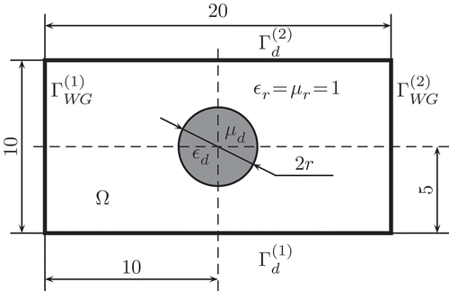
We consider the FE model of a microwave structure, the filter depicted in Figure 1. It consists of a dielectric cylinder of relative electric permittivity and relative magnetic permeability within an air-filled rectangular waveguide. The model features two parameters: the operating frequency GHz and the variation in cylinder radius r. Specifically, we write

(28)

Figure 1. Geometry of rectangular waveguide with dielectric cylinder. All dimensions are in mm.

The FE method leads to a model of the form (1), with explicit frequency-dependence of the system-matrices. The radius variation , on the other hand, turns out to become a non-affine parameter, as a result of geometry discretization.

The authors are aware of the fact that other methods for extracting explicit parameterization for geometric parameters in the FE context are available [11,23]. However, these methods are highly specialized, require non-trivial modifications to the FE solver. To handle more complicated transformations, multiple mappings of subdomains have to be introduced, which may lead to a non-manageable number of coefficients in the parameterization. In contrast, the interpolation approach of Section 4 is very generic and does not require access to the FE kernel. All we need to do is instantiate the FE model at the interpolation points. Note, however, that the FE meshes for different geometrical configurations must be topologically equivalent. We accomplish this with the help of the topology-preserving mesh-deformation method of [28]. One final argument in favour of interpolation is implied by the pMOR method we are using, that is, the single-point algorithm of [12]. For FE systems, which are generally of very large size, single-point methods are particularly efficient, because they require to factorize the system-matrix at one expansion point only. However, single-point methods are restricted to polynomial parameterization, and this is what interpolation delivers naturally. In contrast, the final parameter-dependence produced by the method of [11,23] is of rational type.

In this example, we choose for the interpolation points the zeros of the Tchebychev polynomial of degree 5:

(29)

Our output of interest is the entry of the scattering matrix , which can be computed from the transfer function through

(30)

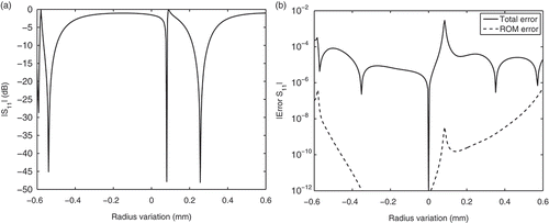
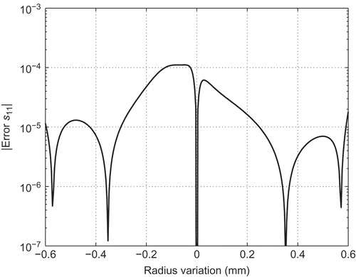
where denotes the identity matrix and is a diagonal matrix that models the frequency dependence ot the wave impedance [29]. Note that, for passive systems, the magnitude of is bounded by one. Figure 2 shows the error introduced by the interpolation step along a line at GHz. It can be seen that the maximum error is in the order of . Also, the five interpolation points are clearly visible.

Figure 2. Magnitude of the error in of the interpolated model with respect to the original FE model as a function of radius variation at GHz.

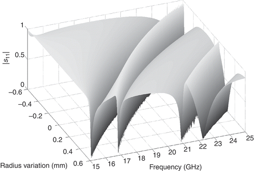
Based on the interpolated model, we construct a moment-matching ROM of order 10 about the expansion point . Figure 3 presents the magnitude of the reflection coefficient as a function of the parameters and . The narrow valleys in the response surface correspond to resonances in the dielectric cylinder. The computational data given in Table 1 demonstrate the great benefit of the proposed order-reduction approach: the speed-up in evaluation time with respect to the interpolated model is 83.

Figure 3. Magnitude of of the ROM as a function of frequency and radius variation .

Table 1. Computational data

	Dielectric post^1		Bandpass filter^2
Example	Interpolated model	ROM	Interpolated model	ROM
Model dimension	5616	132	98472	252
Model generation (s)	167.65	180.71	4019.78	6359.42
Model evaluations per second	3.72	311.31	0.186	298.668
Notes: ^1MATLAB code on Intel T9400 processor, 1 core used.
^2MATLAB code on Intel Xeon E5620 processor, 1 core used.

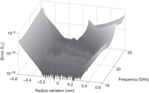
Next, we investigate the error in due to the order-reduction step, with respect to the interpolated model. Figure 4 shows that the MOR error is always below . Over a wide parameter range, it is even much smaller. This confirms the observation of [18] that the interpolation error is dominant.

Figure 4. Magnitude of error in of ROM with respect to interpolated model as a function of frequency and radius variation .

To assess the total error of the combined interpolation/order-reduction method, we consider in Figure 5 a cut through the response surface at GHz. Note that this is the outer edge of the parameter domain associated with the highest frequency value, where the ROM error is expected to be worst. Even there, typical values of the total error are in the range , and the maximum is in the order of , which again confirms the high accuracy of the suggested approach.

Figure 5. System response of ROM and error in as functions of radius variation at GHz.

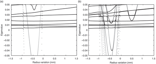
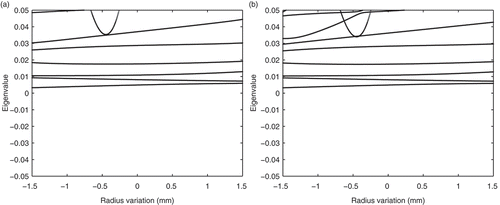
As detailed in Section 4, passivity of the ROM can only be guaranteed when the interpolation step preserves positive (semi-)definiteness of the system matrices. To demonstrate the effects of the two interpolation schemes considered in this article most clearly, we extend the parameter range to mm and place the interpolation points at mm. Figure 6(a) shows that the interpolated stiffness matrix exhibits negative eigenvalues when the naive interpolation approach after Equation (12a) is applied, and Figure 6(b) confirms that negative eigenvalues are also present in the resulting ROM, even though Equations (24)(24) and (25) are used. In contrast, Figure 7(a) shows that the interpolation scheme (21) maintains positive definiteness. Finally, Figure 7(b) demonstrates that the subsequent projection step, based on Equations (24)(24) and (25), preserves definiteness of the reduced-order matrix. The matrices and behave similarly. We omit data. According to Section 4, preservation of (semi-)definiteness implies passivity of the ROM.

Figure 6. Naive interpolation. Smallest eigenvalues of stiffness matrix versus radius variation . Note the presence of negative eigenvalues. (a) Interpolated matrix . (b) ROM:

Figure 7. Interpolation of factorizations. Smallest eigenvalues of stiffness matrix versus radius variation . All eigenvalues are positive and well separated from 0. (a) Interpolated matrix . (b) ROM:

6.2. Bandpass filter

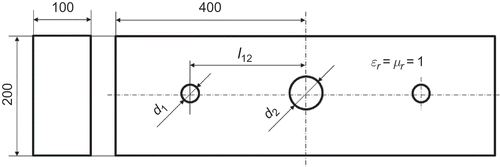
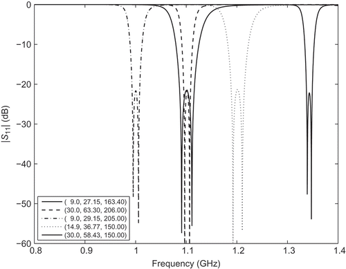
Figure 8 presents a bandpass filter, consisting of three metal rods within an empty rectangular waveguide. The model parameters are given by the diameters of the rods, mm and mm, their distance mm and the operating frequency GHz. As the effect of the geometry parameters on the FE matrix are local, we decouple the various parameter dependencies of the interpolated Cholesky factors (20) and the system matrices (21) by a domain-decomposition approach similar to [27]. For each geometry parameter, we choose the zeros of the Tchebychev polynomial of degree 7 as interpolation points. At the order-reduction step, we build a moment-matching ROM of order 5 about the expansion point . 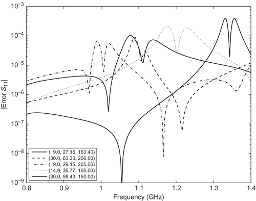The ROM allows to construct a whole family of 20 dB bandpass filter of greatly varying bandwidth and centre frequency. Figures 9 and 10 present the reflection coefficient as well as the combined interpolation and order-reduction error for different filter configurations. It can be seen that the error is always below . Table 1 demonstrates the benefit of the pMOR method: by reducing the model dimension from almost 100,000 to 252, order reduction accelerates the evaluation of the model by more than four orders of magnitude.

Figure 8. Geometry of bandpass filter. All dimensions are in mm.

Figure 9. Magnitude of as a function of frequency for selected filter configurations, computed by pMOR. Parameters of legend denote in mm. Number of evaluation frequencies = 2001.

Figure 10. Total ROM error in as a function of frequency with respect to full FE solutions. Parameters of legend denote in mm. Number of evaluation frequencies = 201.

7. Summary and outlook

We have investigated an important class of parameter-dependent LTI systems that arises in applications as diverse as dynamic analysis of mechanical structures, circuit simulation of RLC networks and computational electromagnetics. We have first proved passivity, causality and reciprocity and then, as the main contribution of this article, proposed a novel method of model-order reduction that preserves these properties even in the presence of non-affine parameters. Its key ingredients are a new interpolation procedure and a modified projection approach. Future applications will include shape optimization and inverse problems.

References

- Amsallem , D. , Cortial , J. , Carlberg , K. and Farhat , C. 2009 . A method for interpolating on manifolds structural dynamics reduced-order models, Int . J. Numer. Methods Eng. , 80 ( 9 ) : 1241 – 1258 .
- Panzer , H. , Mohring , J. , Eid , R. and Lohmann , B. 2010 . Parametric model order reduction by matrix interpolation . Automatisierungstechnik , 58 ( 2 ) : 475 – 484 .
- Baur , U. and Benner , P. 2009 . Modellreduktion für parametrisierte Systeme durch balanciertes Abschneiden und Interpolation . Automatisierungstechnik , 57 ( 8 ) : 411 – 419 .
- Gunupudi , P. , Khazaka , R. and Nakhla , M. 2002 . Analysis of transmission line circuits using multidimensional model reduction techniques . IEEE Trans. Adv. Packag. , 25 ( 2 ) : 174 – 180 .
- Weile , D.S. , Michielssen , E. , Grimme , E. and Gallivan , K. 1999 . A method for generating rational interpolant reduced order models of two-parameter linear systems . Appl. Math. Lett. , 12 : 93 – 102 .
- Weile , D.S. and Michielssen , E. 2001 . Analysis of frequency selective surfaces using two-parameter generalized rational Krylov model-order reduction . IEEE Trans. Antennas Propag. , 49 : 1539 – 1549 .
- Daniel , L. , Ong , C.S. , Chay , L.S. , Lee , K.H. and White , J. 2004 . A multiparameter moment-matching model-reduction approach for generating geometrically parameterized interconnect performance models . IEEE Trans. Comput. Aided Des. Integr. Circuits Syst. , 23 : 678 – 693 .
- Codecasa , L. 2005 . A novel approach for generating boundary condition independent compact dynamic thermal networks of packages . IEEE Trans. Compon. Packag. , 28 : 593 – 604 .
- Li , Y.-T. , Bai , Z. , Su , Y. and Zeng , Z. 2008 . Model order reduction of parameterized interconnect networks via a two-directional Arnoldi process . IEEE Trans. Comput. Aided Des. Integr. Circuits Syst. , 27 ( 9 ) : 1571 – 1582 .
- Prud'homme , C. , Rovas , D.V. , Veroy , K. , Machiels , L. , Maday , Y. , Patera , A.T. and Turinici , G. 2002 . Reliable real-time solution of parametrized partial differential equations: reduced-basis output bound methods . J. Fluids Eng. , 124 : 70 – 80 .
- Rozza , G. , Huynh , D.B.P. and Patera , A.T. 2008 . Reduced basis approximation and a posteriori error estimation for affinely parameterized elliptic coercive partial differential equations . Arch. Comput. Meth. Eng. , 15 : 229 – 275 .
- Farle , O. and Dyczij-Edlinger , R. Numerically stable moment matching for linear systems parameterized by polynomials in multiple variables with applications to finite element models of microwave structures . IEEE Trans. Antennas Propag. 58 (11) (2010), pp. 3675–3684 ,
- Freund , R.W. 2005 . “ Padé-type model reduction of second-order and higher-order linear dynamical systems ” . In Dimension Reduction of Large-Scale Systems , Edited by: Benner , P. , Sorensen , D.C. and Mehrmann , V. 191 – 223 . Berlin, Heidelberg : Springer .
- Tisseur , F. and Meerbergen , K. 2001 . The quadratic eigenvalue problem . SIAM Rev. , 43 : 235 – 286 .
- Webb , J.P. and Parihar , S. 1985 . Finite element analysis of H-plane rectangular waveguide problems . IEE Proc. , 133 : 91 – 94 .
- Barrault , M. , Maday , Y. , Nguyen , N.C. and Patera , A.T. 2004 . An ‘empirical interpolation’ method: application to efficient reduced-basis discretization of partial differential equations . C.R. Acad. Sci. Paris Ser. I , 339 : 667 – 672 .
- Grepl , M.A. , Maday , Y. , Nguyen , N.C. and Patera , A.T. 2007 . Efficient reduced-basis treatment of nonaffine and nonlinear partial differential equations . Math. Modell. Numer. Anal. (M2AN) , 41 : 575 – 605 .
- Dyczij-Edlinger , R. and Farle , O. 2009 . Finite element analysis of linear boundary value problems with geometrical parameters . COMPEL , 28 : 779 – 794 .
- Vlach , J. and Singhal , K. 1993 . Computer Methods for Circuit Analysis and Design , 2nd , New York : John Wiley & Sons .
- Dyczij-Edlinger , R. and Biro , O. 1996 . A joint vector and scalar potential formulation for driven high frequency problems using hybrid edge and nodal finite elements . IEEE Trans. Microwave Theory Tech. , 44 : 15 – 23 .
- Pozar , D.M. 1998 . Mivrowave Engineering , 2nd , New York : John Wiley & Sons .
- Triverio , P. , Grivet-Talocia , S. , Nakhla , M.S. , Canavero , F.G. and Achar , R. 2007 . Stability, causality, and passivity in electrical interconnect models . IEEE Trans. Adv. Packag. , 30 : 795 – 808 .
- Moosmann , C. 2007 . ParaMOR – Model order reduction for parameterized MEMS applications, Ph.D. diss , Albert-Ludwigs-Universität Freiburg .
- Haasdonk , B. , Ohlberger , M. and Rozza , G. 2008 . A reduced basis method for evolution schemes with parameter-dependent explicit operators . Electron. Trans. Numer. Anal. , 32 : 145 – 161 .
- Chaturantabut , S. and Sorensen , D.C. 2010 . Discrete empirical interpolation for nonlinear model reduction . SIAM J. Sci. Comput. , 32 ( 5 ) : 2737 – 2764 .
- Davis , P.J. 1975 . Interpolation and Approximation , 24 – 94 . New York : Dover Publications .
- Selleri , S. , Farle , O. , Guarnieri , G. , ösch , M. L , Pelosi , G. and Dyczij-Edlinger , R. 2008 . A combined domain decomposition – model order reduction technique for fast finite element parametric sweep . IEEE Antennas Propag. Symp. Dig. , 1–9 : 2010 – 2013 .
- Burgard , S. 2008 . Morphing von Finite-Elemente-Netzen, Studienarbeit, Lehrstuhl für Theoretische Elektrotechnik, Universität des Saarlandes
- Rubio , J. , Arroyo , J. and Zapata , J. 2001 . SFELP – An efficient methodology for microwave circuit analysis . IEEE Trans. Microwave Theory Tech , 49 ( 3 ) : 509 – 516 .