Optimal filtering of piecewise deterministic processes for source detection and separation in electric load monitoring

Abstract

We wish to compute in discrete real time the best estimate for the composition of the total active power recorded at a customer's house, without any intrusion. A new solution for online characterization of the electric load is proposed. The solution is based on issues from the applied stochastic analysis of Markov processes. We specifically suggest that optimal filtering of a hybrid stochastic differential system covers entirely the detection and separation subproblems underlying the main problem.

Keywords:

• electric load monitoring
• hybrid stochastic differential systems
• piecewise deterministic processes
• Fokker–Planck equation
• non-linear filtering

1. Introduction

Saving energy is a challenge for the industry and the consumers of electricity for economic and environmental reasons. Compiling electric load data turns consumers' variable electric appliances and habits from a source of confusion to a source of knowledge. This is what the experts call electric load monitoring, namely, using the electricity meter. This tool is a centralized and accessible part of a distribution network. We are primarily concerned here with understanding the electric load by separating (or isolating) its major components; their number is of course unknown since it is random and varying in time. In principle, such a problem is dealt with as two subproblems: (1) detection – estimating the number of components; and (2) decomposition – estimating the bearings of those components. Here we shall not make this distinction; we address at one go these two problems. Our approach is to formulate the basic problem as filtering a hybrid stochastic differential system.

The literature on source detection and separation is extensive; see, for example, the book by Johnson and Dudgeon [1]. This leads us to a general classification of possible methods into two categories depending on whether the number of sources is known a priori. In any case, the number of sources is determinate and fixed during the observation. Regarding the application, among the basic references concerning electric load monitoring are [2–4], but the work by El Guedri [5] is our key source reference. Her algorithm in [6], for instance, is based on the interpretation of the convector signature in the time-frequency domain. It appears, however, that again the unknown number of convectors is assumed to be fixed throughout the experimental tests. It may be more realistic to regard this number depending on time as random variable. Indeed, this is precisely the discrete component of our hybrid stochastic differential system.

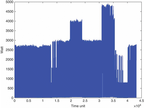
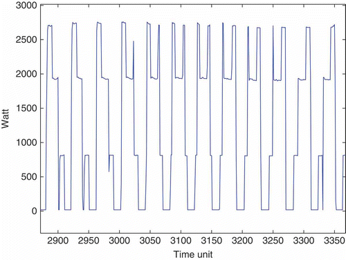
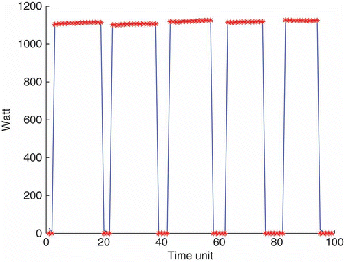
The treatment here, and in the references mentioned above, is focused on space heating by convectors since it is the most consuming appliance. The active power sample path of a heating load for 1 day is plotted in Figure 1; Figure 2 is a zoom in this plot. Certain assumptions must be made about the underlying signals; to this end, an example of a signal generated by one convector is shown in Figure 3. This plot reveals, for instance, a time variation of the width of squares due to a saturation of the convector. For this argument, we assume that the observed signal is a sum of a time-varying random number – which may be null – of possibly overlapping squares. It is worth noting that a square amplitude may be the same even if it corresponds to different convectors. Besides, a synchronism between two convectors is frequent: the start up of a square and the shutdown of another occur at the same time. All these aspects are taken into account by the following model and shall not be sources of complexity anymore.

Figure 1. A sample path of space heating for 1 day.

Figure 2. Zoom in the sample path plotted above.

Figure 3. A sample path for only one convector.

Let y_t be the number of squares at time t and x_t the vector of amplitudes of these squares. In other words, when y_t ≠ 0, it represents the dimension of x_t . Moreover, as long as y_t  = 0, x_t  = 0. A sample path of y_t is thus a step function assuming values in a finite discrete set, say {0,1,2,3}. Here, this means that there must not be more than three convectors that are simultaneously on at any time. Let t = 0 on starting the observation of any heating load. The observation z_t is the sum of the components of x_t if y_t ≠ 0, that is,

But as long as y_t  = 0, the observation z_t is null. Finally, we assume that at t = 0, y ₀ = 0 and thus x ₀ = 0, z ₀ = 0.

Section 2 is devoted to the development of a model for the unobservable, or latent, signal (x_t , y_t ): a piecewise deterministic process (PDP). The ingredients of the PDP – such as the state space, the vector field – are then identified from real data. Thus, characterizing the electric heating load is nothing but filtering the PDP (x_t , y_t ) from the observable process z_t . Of interest are a couple of operators associated to any Markov process: the generating operator and the Fokker–Planck operator. Section 3 consists of the computation of these bearings for our signal model, the PDP (x_t , y_t ). Section 4 contains the filtering equations and a demonstration on real data provided by Électricité de France.

2. A hybrid stochastic differential system: PDP

A piecewise deterministic process is one particular determinate motion that starts afresh between random jumps of two kinds, spontaneous or predictable. Jumping has two ingredients: a hazard rate for spontaneous jumps and a probability distribution to reinitiate the motion after every jump, of both types. This results in a strong Markov càdlàg stochastic process. PDP has widely been used since Davis introduced it in 1984; the reference [7] is our main tool on the subject.

State space E: The state space of a PDP is a disjoint union of some manifolds with boundary.

where Y is a space with discrete topology. For each y ∈ Y, M_y is an open set from IR ^d(y), here d is a function on Y into .

Thus, a PDP is denoted as (x_t , y_t ) or ξ _t with ; y_t is a Y-valued continuous-time process and x_t is a continuous-time process with values in M_y as long as y_t  = y × y_t is assumed as the discrete component of the state and x_t its continuous component.

Remark. As a Markov process, ξ _t is based on some filtered probability space . Customarily, a family of probability measures on is defined by

By construction

Under the original probability measure IP, ξ _t starts at t = 0 with μ, a probability distribution on , where is the Borel σ-algebra of E. For the simple reason that

one uses sometimes the notation IP_μ for the original probability measure. One shall freely work in all these probability measures.

Vector field Φ: One particular vector field determines the motion between the jumps. Denote the first jump time of ξ _t as T ₁. Then

c(t) is the integral curve (or flow) of a vector field Φ at x, that is, a map such that

Jumping rate λ: T ₁ is a random variable with the following probability distribution:

where is the instant at which the flow c starting at x reaches the boundary ∂M_y ; if this never occurs.

Active boundary Γ: Starting from any interior point, everywhere a PDP reaches the boundary ∂E it jumps instantaneously. Thus, the active or essential boundary of the state space is the set of boundary points almost surely reachable by the process (within a predictable stopping time). This is also written as: the active boundary Γ is a set of boundary points of the state space such that

Markovian kernel Q: It states the conditional probability distribution on E of the post-jump state ξ(T ₁) given the conditioning event

for , that is,

for Λ a Borel-measurable set from E, without regard to the probability measure under which this probability is computed.

Further into the application

Let us finish the modelling that we have began in the introduction by identifying the ingredients of our PDP. Here there are four regimes or modes labelled by the number of squares, that is,

As long as y_t  = 1, x_t is the square amplitude taking values in and solving

The square magnitudes A _min, A _max are the lower and upper bounds of the nominal power for any convector; these are known from real data [5]:

As long as y_t  = 2, x_t takes values in and solves

The same reasoning holds for the fourth regime, as and when y_t  = 3. Thus, the vector field within the non-degenerate modes (modes 1,2 and 3) is null,

It is clear that the state space is given by

and that for any , it follows that the essential boundary Γ = Ø.

Jumping between the regimes or within one and the same regime is done in the following way:

•	From mode 0, a jump goes to modes 1, 2 or 3, with the same probability of 1/3 each. Furthermore, we assume a jumping rate λ0 constant over time.
•	There may be jumps of our PDP within mode 1 – these are jumps of its continuous component – or jumps from mode 1 to modes 0, 2 or 3. We assume the same probability of 1/4 for each kind of jumps, and a constant jumping rate λ1.
•	The reasoning for mode 1 applies to modes 2 and 3 with jumping rates λ2 and λ3, respectively.

As to the Markovian kernel, we make this choice: the process ξ _t is reinitiated according to a uniform distribution after every jump to a non-degenerate mode, that is, for any (x, y) ∈ E

(1)

Note the independence from the pre-jump state ξ = (x, y). Obviously, for jumps to mode 0, we have for any

3. The generating operator and the Fokker–Planck operator for the signal model

The above description yields, in the first place, to the generating operator of our signal model, the PDP ξ _t . Let f be a measurable function and we claim that

where obviously

For x ∈ M ₁,

For x ∈ M ₂,

For x ∈ M ₃,

There are no imposed conditions on – the domain of – at the boundary of the state space since this boundary is never reached.

Now we are ready to write Dynkin's formula for the signal process ξ _t . Dynkin's formula is the main tool in computing expectations for a wide class of functions:

provided that f is bounded and the mean number of entering/exiting squares per finite time interval is finite [8]; this holds quite naturally in our application.

In the second place, the central concept of this section is the Fokker–Planck operator along with its domain . It is the adjoint of the generating operator in the sense that, for and ,

The pairing of and p, regarded as a function of x, denotes

and denotes

Note that to write the relations above, we need to assume the existence of a density p(t, x, y) or p(t, ξ) for the distribution on , under IP, of . That is, for y ∈ Y, y ≠ 0, and Λ a Borel-measurable set from M_y

We claim that for x ∈ M ₁,

For x ∈ M ₂,

For x ∈ M ₃,

Assuming that for each and each y ∈ Y, y ≠ 0, possesses a density with respect to the Lebesgue measure on M_y , written

and in view of Equation (1)(1), it follows that for each

Thus, for x ∈ M ₁,

For x ∈ M ₂,

For x ∈ M ₃,

Finally, we claim that

where, for homogeneity of notation, we set

Regarding , it is the set of functions satisfying for each

Furthermore, there are no imposed conditions on p – so as to belong to – at the boundary of the state space since this boundary is never reached by the process ξ _t .

Now if we assume that

(2)

we obtain

The assumption (Equation (2)(2)) is not an artefact to simplify the calculus; it says that we do not have any reason to attest that all the kinds of jumps do not have the same rate or intensity. A straightforward calculation based on real data shows that

Finally, the distribution density of ξ _t solves the Fokker–Planck equation [9](9):

with the initial condition

The solution of the Fokker–Planck equation above is given by

4. Filtering

Now we consider the filtering problem associated to the couple (ξ _t , z_t ). We have non-linear observations of ξ _t , the discrete-time process (z_n ) _{n = 1, 2, …} indexed at irregularly spaced instants t ₁, t ₂, …; these are deterministic and known. The observations are related to the state process via the conditional distribution

for Λ a Borel-measurable set from . For homogeneity of notation, we set t ₀ = 0 so that . While not essential, it is convenient to give a small perturbation to the observations so as to account for measurement errors, if any: When y(t_n ) ≠ 0,

but if y(t_n ) = 0, x(t_n ) = 0 and

where ε is a small positive number and {w_n } _{n = 1, 2, …} is a Gaussian white noise with null mean and unit variance. Again, in view of real data, we may take ε = 10 Watts. Finally

It appears clearly now that the perturbation is also done so as to avoid the Dirac measure when expressing the conditional distribution in the filtering equations; see Equations (10)(10) and (11)(11).

4.1. Conditional density characterization: the optimal filter

The best estimate – in a sense of the mean square – of f(ξ _t ) given the observations up to time t is the conditional expectation

for all reasonable functions f on E. Assume the existence of a density for the distribution

where y ∈ Y, y ≠ 0, and Λ is a Borel-measurable set from M_y , that is,

For homogeneity of notation, we set

Now recall the Fokker–Planck operator of ξ _t developed in Section 3; it follows that the posterior distribution density for t_{n –1} ≤ t < t_n , n ≥ 1, solves the Fokker–Planck equation

(3)

with the initial condition

(4)

Here analytic resolution of Equations (3(3) –4(4)) is computationally tractable. The solution is 5–8) below:

(5)

(6)

(7)

(8)

On the other hand, at each observation instant t_n , n ≥ 1, solves the Bayes rule

(9)

where is the solution of Equations (3(3) –4(4)) as t ↑ t_n , and

(10)

(11)

Obviously, the initialization of the optimal filter is given by

The symbol ∝ in Equation (9)(9) means up to a normalization constant. This constant is computed by imposing the following condition at each observation time t_n , n ≥ 1:

Then looking at 5–8), one can easily see that the condition

holds also for each t, t_{n –1} < t < t_n , n ≥ 1.

4.2. Implementation result

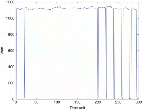
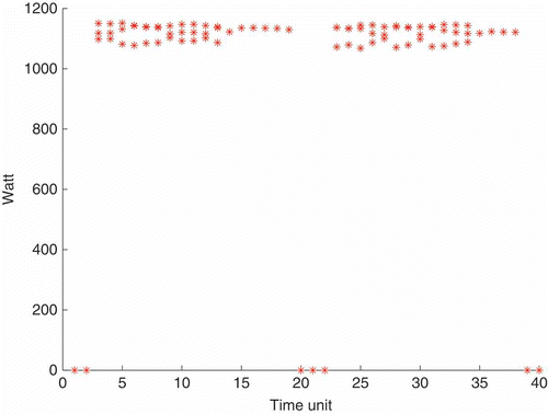
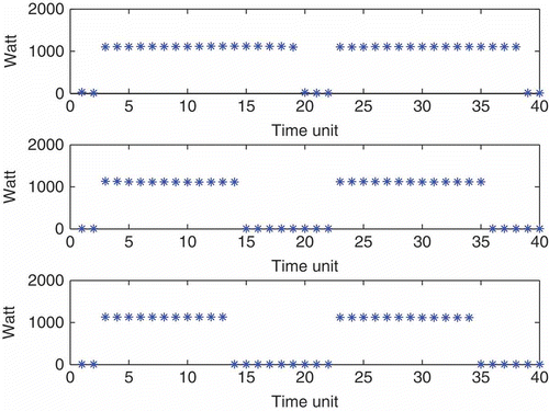
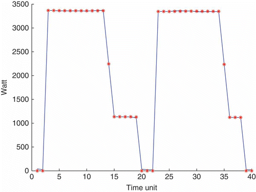
A run on a synthetic mixture is displayed in Figure 4; Figure 5 shows the true mixture components. The observed signal which is the filter input is, of course, the sum of these components, and Figure 5 is useful as a reference. At each observation time the set of stars is the a posteriori maximum estimate of the state , n ≥ 1. Note the accuracy of the decomposition: the number of squares is recovered and the magnitudes of these squares are quite well estimated. Figure 6 is to check if the summation (stars) of the component magnitudes coincide with the observation (full line). A second run on another scenario is displayed in Figure 7 where we plot the reference (full line), which is also the observed signal, and the estimate (stars).

Figure 4. The filter output. The mixture components are detected and separated.

Figure 5. The true mixture components. The observed signal is the sum of these components.

Figure 6. The sum of the estimated mixture components versus the observed signal.

Figure 7. A second run on a sample path of one convector.

5. Conclusion and future work

Probabilistic management of uncertainty in dynamical systems is addressed with application in electric load monitoring. We sum up the contribution of this article by: a non-intrusive method for characterizing the space heating. This is based on modelling the underlying signals as a hybrid stochastic differential system. Thus the characterization is reformulated as a filtering problem. The optimal filter is computed and then implemented with real scenarios. Comparisons are made, and the apparent usefulness of the method is assessed. It must be borne in mind, however, that optimal filtering is possible only if the analytic resolution of the Fokker–Planck equation is feasible. It should be emphasized that whereas the treatment here is based on the interpretation of the convector signature – a square – in the time domain, our method has wider applicability. On the one hand, it extends to more general problems of source detection and separation; and on the other, it applies to other electric appliances. In this connection, another appliance may have a different signature but leads us again to a vector field which is then not null and, of course, the same for all the non-degenerate modes.

References

- Johnson , D.H. and Dudgeon , D.E. 1993 . Array Signal Processing: Concepts and Techniques , Englewood Cliffs, NJ : Prentice-Hall .
- Hart , G. 1989 . Residential energy monitoring and computerized surveillance via utility power flows . IEEE Technol. Soc. , 8 ( 2 ) : 12 – 16 .
- Laughman , C. , Lee , K. , Cox , R. , Shaw , S. , Norford , L. and Armstrong , P. 2003 . Power signature analysis . IEEE Power and Energy Mag. , 1 ( 2 ) : 55 – 63 .
- Leeb , S. 1993 . A conjoint pattern recognition approach to non-intrusive load monitoring , Ph.D. diss., Massachusetts Institute of Technology .
- El Guedri , M. 2009 . Caractérisation aveugle de la courbe de charge électrique: détection, classification et estimation des usages dans les secteurs résidentiel et tertiaire , Ph.D. diss., Université Paris Sud IX .
- El Guedri , M. Time frequency characterization for electric load monitoring . 17th European Signal Processing Conference . Glasgow, Scotland. CD-ROM Proceedings, 08/09 .
- Davis , M.H.A. 1993 . Markov Models and Optimization , London : Chapman & Hall .
- Baili , H. 2011 . Stochastic analysis of noncompliance with drug therapy . J. Uncertain. Syst. , 5 : 38 – 44 .
- Gardiner , C.W. 1985 . Handbook of Stochastic Methods for Physics, Chemistry and the Natural Sciences , 2nd , Berlin : Springer-Verlag .