Environment-driven distributed evolutionary adaptation in a population of autonomous robotic agents

Abstract

This article is concerned with a fixed-size population of autonomous agents facing unknown, possibly changing, environments. The motivation is to design an embodied evolutionary algorithm that can cope with the implicit fitness function hidden in the environment so as to provide adaptation in the long run at the level of population. The proposed algorithm, termed mEDEA, is shown to be both efficient in unknown environments and robust to abrupt and unpredicted changes in the environment. The emergence of consensus towards specific behavioural strategies is examined, with a particular focus on algorithmic stability. Finally, a real-world implementation of the algorithm is described with a population of 20 real-world e-puck robots.

Keywords:

• evolutionary robotics
• artificial life
• open-ended evolution
• swarm intelligence

1. Introduction

With the advent of reliable and powerful software and hardware at reasonable cost, it is now possible to study the dynamics of large groups of autonomous agents within various environments. Indeed, much work has already addressed the issue of designing efficient adaptive behavioural strategies in populations of agents, with very different approaches and motivations [1,2]. One particularly interesting scenario is a population of robotic units that is immersed in a completely unknown environment, yet still manages to survive, then moves into a different environment requiring very different behavioural strategies. In this article, we are interested in a fixed-size population of autonomous physical agents using local communication, such as autonomous robots, facing unknown and/or dynamic environments. This class of problems typically applies when the environment is unknown to the human designer until the population of agents is actually made operational in the real situation [3], or whenever the environment is expected to change during operation with no indication of when and how these changes will impact survival strategies.

The challenge is to design a distributed online optimization algorithm addressing agent self-adaptation in the long term, that is, able to successfully manage an implicit pressure resulting from environmental properties and algorithmic constraints with regard to the optimization process. While the lack of explicit objective function is a major characteristic of the current problem setting, several ideas may be drawn from closely related fields. In particular, reinforcement learning in decentralized systems has been extensively studied and it is well known that such problems are notoriously difficult (e.g. decentralized partially observable Markov decision process is NEXP-complete [4]), and approximate solving methods stand as the only pragmatic option. In this scope, direct policy search [5–7] is a powerful alternative based on directly optimizing policies (i.e. behavioural strategies) of agents. Moreover, evolutionary algorithms stand as a powerful tool for direct policy search due to flexible representation and stochastic operators and have been shown to be a competitive approach in the face of uncertainty and partially observable tasks in large dimensions [8,9]. However, traditional evolutionary robotics (ER) requires that evolutionary optimization is performed before the actual use of a solution, not during exploitation. The question is then how to perform evolutionary optimization online.

Embodied evolution (EE), as proposed initially in [10], addresses part of this question as it focuses on algorithms for evolutionary optimization of agent behaviours in an online, possibly decentralized, manner. To some extent, EE can be seen as a specific flavour of online learning algorithm as the original motivation is to embed evolutionary optimization algorithms within the population of robotic agents. In this set-up, the problem of noisy evaluations due to the lack of control over the initial conditions is explicitly addressed and the evolutionary algorithm implementation resembles an island-based model, where each robotic agent executes an onboard evolutionary algorithm, possibly exchanging genomes from one agent to another whenever communication range permits. A few references have explored this set-up in the last 10 years ([11–14] among others), including previous work from the authors [15,16]. Unfortunately, EE requires an objective function designed by the supervisor, which is unavailable by definition in the problem setting addressed in this article. Indeed, the absence of an objective function provides a significant challenge that has seldom been studied. ¹

While concepts and methods from EE may be relevant, we can only assume that maximizing the integrity of the agent population as well as maintaining a communication network for exchanging genomes are the basic requirements in the present context. To this end, we propose a distributed algorithm for environment-driven self-adaptation based on evolutionary operators that takes into account selection pressure from the environment. The thinking behind this algorithm is to consider the strategies as the atomic elements and the population of agents as a distributed substrate on which strategies compete with one another. This approach is better illustrated using the selfish gene metaphor [22]: one specific strategy (or set of parameters, or genome) is ‘successful’ if it manages to spread across the population, which implicitly requires it to both minimize the risk for its ‘vehicles’ (i.e. the autonomous agents) and maximize the number of mating opportunities, although the two may be contradictory.

The overall motivation behind the work presented here is the study of general evolutionary adaptation algorithms that can ultimately be implemented on real robotic hardware. To this end, the main contribution of this article is a novel distributed evolutionary adaptation algorithm for use in a population of autonomous agents (Section 2) and experimental validation with regard to robustness of the algorithm to unknown, and changing, environments, under realistic constraints (fixed number of agents, limited sensors, actuators, etc.) (Section 4). The dynamics of evolutionary adaptation is also studied, with a particular emphasis on the emergence of consensus around a given behavioural strategy (Section 5). Finally, the implementation of the algorithm within a population of real robots illustrates a practical implementation problem in Section 6.

2. Environment-driven distributed evolutionary adaptation

As stated in Section 1, our objective is to design a distributed online evolutionary algorithm for a fixed population of autonomous physical agents (e.g. autonomous robots) that can cope with environmental constraints and learn to survive in the long term. It follows that the key to environment-driven distributed evolutionary adaptation (EDEA) is the implicit nature of the fitness function. However, this implicit fitness may be seen as the result of two possibly conflicting motivations:

•	extrinsic motivation: an agent must cope with environmental constraints in order to maximize survival, which results solely from the interaction between the agent and its environment (possibly including other agents); and
•	intrinsic motivation: a set of parameters (i.e. ‘genomes’) must spread across the population to survive, in accordance with the algorithmic nature of the evolutionary process. Therefore, genomes are naturally biased towards producing efficient mating behaviours as the larger the number of agents met, the greater the opportunity to survive.

The level of correlation between these two motivations impacts problem complexity to a significant degree: a high correlation implies that the two motivations may be treated as one while a low correlation implies conflicting objectives. An efficient EDEA algorithm must address this trade-off between extrinsic and intrinsic motivations as the optimal genome should reach the point of equilibrium where genome spread is maximum (e.g. looking for mating opportunities) with regard to survival efficiency (e.g. ensuring energetic autonomy).

These questions have been extensively studied in the field of open-ended artificial evolution with an emphasis on computational models of evolutionary dynamics [18], including a particular focus on the effect of the environment on the evolutionary adaptation process [23]. However, their application within EE is still an open issue as EE is concerned with a fixed number of physically grounded agents that are intended to operate in real-world environments (e.g. subject to obstacles, energy constraints).

2.1. MEDEA: a minimal EDEA algorithm

Based on these considerations, we introduce the mEDEA (minimal EDEA) algorithm, described in Algorithm 1. This algorithm describes how evolution is handled on a local basis and the same algorithm is executed within all agents in the population. The algorithm runs alongside a communication routine whose purpose is to receive incoming genomes and store them in the imported genome list for later use.

At a given moment, a given agent is driven by a control program whose parameters are extracted from an ‘active’ genome which remains unchanged for a generation. This genome is continuously broadcast to all agents within (a limited) communication range. This algorithm implements several simple but crucial features that can be interpreted from the viewpoint of a traditional evolutionary algorithm structure:

Selection operator: the selection operator is limited to simple random sampling among the list of imported genomes, that is, no selection pressure on a local individual basis. In fact, selection pressure is active at the global level (population) rather than at the local level (individual): the most widespread genomes on a global population basis are more likely to be randomly sampled on average. Indeed, the algorithm benefits from the large population with many mating opportunities.

Algorithm 1 The mEDEA algorithm

genome.randomInitialize()

while forever do

 if genome.notEmpty() then

  agent.load(genome)

 end if

 for iteration = 0 to lifetime do

  if agent.energy > 0 and genome.notEmpty() then

   agent.move()

   broadcast(genome)

  end if

 end for

 genome.empty()

 if genomeList.size > 0 then

  genome = applyVariation(select _random(genomeList))

 end if

  genomeList.empty()

end while

	Variation operator: the variation operator is chosen to be rather conservative to ensure continuity during the course of evolution. Generating altered copies of a genome only makes sense if there is some continuity in the genome lineage: with no variation the algorithm will simply converge on average towards the best genome initially existing in the population. In the following, we assume a Gaussian random mutation operator, inspired by evolutionary strategies [24], with which the locality of mutation can be easily tuned through a parameter.
	Replacement operator: finally, replacement of the current active genome to control a given agent is achieved by (1) local deletion of the active genome at the end of one generation and (2) randomly selecting a new active genome among the imported genome list (cf. selection operator). On a population level, this implies that surviving genomes are likely to be correlated with efficient mating strategies, as a given genome will only survive in the long run through more or less slightly different copies of itself.
	The positive or negative impact of environmental variability on genome performance is smoothed by the definition of the variation operator, as newly created genomes are always more or less closely related to their parent. As a consequence, genotypic traits result from a large number of parallel evaluations, both on the spatial scale as closely related copies sharing the same ancestor may be evaluated in a population and on the temporal scale as any one genome is also strongly related to its ancestors. Hence, a single genome may be picked by chance once in a while, but it is highly unlikely that a ‘family’ of closely related genomes manages to survive in the population if there are more efficient competitors. Moreover, the larger the population, the lower the sampling bias: in other words, better than average genomes will get a better chance of surviving if the population is large.
	A fundamental requirement for ensuring selection pressure is that there is a strict constraint on the maximum number of genomes to choose from during selection with regard to the population size . must hold for at least one agent (i.e. the received genome list should contain strictly less than all genomes from the population minus the local genome). Otherwise, no selection pressure will apply as genome survival probabilities would be uniform over the swarm. Then again, this worst-case scenario does not necessarily imply failure of the algorithm: the lack of selection pressure implies random walk in the genotypic space thanks to the variation operator (i.e. random genetic drift [25]), possibly leading to a new -- possibly more interesting -- region of the genotypic space, at the cost of temporary loss of selection pressure.

3. Representation/encoding the problem

Specifications for the autonomous agents are inspired by a traditional robot configuration, with eight proximity sensors arranged around the agent body and two motor outputs (translational and rotational speeds). Three additional sensory inputs are considered: the angle and distance towards the nearest food item and the current energy level. Each agent is controlled by a multi-layer perceptron (MLP) with five hidden neurons, which means a total of 72 weights. ² Note that the mEDEA algorithm is independent of any particular control architecture implementation, even though artificial neural networks provide a convenient, flexible and well-established representation formalism. Thus, in experiments, we will focus on the dynamics of the mEDEA algorithm rather than providing in-depth analysis of the particular internal properties of the evolved neural networks.

The variation operator is a Gaussian mutation with one parameter: a small (respectively, large) tends to produce similar (respectively, different) offspring. This is a well-known scheme from evolution strategies where continuous values are solely mutated using parameterized Gaussian mutation, where the parameter may be either fixed, updated according to predefined heuristics, or evolved as part of the genome. In the scope of this work, we rely on self-adaptive mutation where is part of the genome [24] (i.e. the full genome contains 73 real values).

As with other genome parameters, the value responds to environmental pressure: a genome survives in the population if it leads to efficient agent behaviour and if it is able to produce comparable or fitter offspring. In some cases, this requires a fine tuning of existing genome parameters (i.e. local search), while in other cases it requires very different genomes (i.e. escaping local optima).

The current implementation of the update rule is achieved by introducing , a update value, which is used to either decrease () or increase () the value of whenever a genome is transmitted. In the following, is a predefined value set prior to the experiment so that it is possible to switch from the largest (respectively, smallest) value to the smallest (respectively, largest) in a minimum of approximately 9 (respectively, 13) iterations (i.e. there is a bias towards local search).

4. Experiment #1: robustness to environmental change

This section provides a description of the experimental setting and implementation details. The motivation here is to design a setting such that it is possible to address several issues regarding evaluation and validation of the proposed algorithm. In particular, the robustness of mEDEA to environmental pressure and sudden environmental changes will be studied.

4.1. The problem: surviving in a dynamic unknown environment

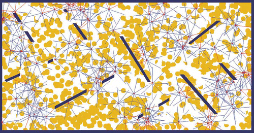
Figure 1 shows the environment used for experiments: a 2D arena with obstacles, possibly containing food items. The figure also illustrates 100 autonomous mobile agents loosely based on the e-puck mobile robot specification. This environment is used for two different experimental set-ups, described as follows:

Figure 1. Snapshot from the simulator with 100 agents. Food items are represented as circles. Agents are represented with proximity sensor rays, modelled on the e-puck robot. Communication range is half the range of proximity sensors.

1.

the ‘free-ride’ set-up • Description: a population of autonomous mobile agents is placed in an environment with few obstacles. As the agent's active genome is automatically deleted at the end of the current generation, a robotic agent is active in the next generation only if at least one new genome is available (i.e. if the agent was able to meet with at least one other agent). • Motivation: this set-up makes it possible to evaluate the mechanisms of the mEDEA algorithm as environmental pressure should be limited.

2.

the ‘energy’ set-up • Description: energy resources (‘food items’) are spread throughout the environment and these can be harvested by the agents. Agents have an energy level, which depends on harvested food items and power consumption. If the energy level reaches 0, the agent halts and the genome is lost. Harvested food items only ‘grow’ back after a given number of iterations. • Motivation: in this set-up genomes also compete for agent resources but have to deal with environmental pressure as maximizing mating encounters may not be compatible with energy self-sustainability.

The full experimental set-up considers starting with the ‘free-ride’ set-up and then abruptly switching to the ‘energy’ set-up after a predefined fixed number of generations. Agents are of course unaware of such a change in the environment and continue to run the same unchanged mEDEA algorithm. The motivation behind this sequential switch from one set-up to another is to evaluate mEDEA robustness to environment change, which is a desirable feature of all online learning/optimization algorithms.

4.2. Experimental settings

The whole experiment lasts for 150 generations, switching from the ‘free-ride’ set-up to the ‘energy’ set-up at generation 75. As said before, the energy level is not used during the ‘free-ride’ set-up – the additional sensor values related to energy points are thus useless in this set-up and may even be considered as distractions. During the course of evolution, some agents may come to a halt either because they did not meet any other agents (in both set-ups), thus failing to import a new genome for use in the next generation, or because they ran out of energy during the ‘energy’ set-up (each agent can store a maximum of 400 energy units and consumes 1 unit/step, one generation lasts 400 steps, each harvested food item gives 100 units of energy). In the ‘free-ride’ set-up, the agents without a genome remain still (or ‘inactive’, i.e. without genome), waiting for new genomes imported from ‘active’ agents that eventually come into contact. ³ In the ‘energy’ set-up, these agents remain stationary until the end of the current generation after which they are automatically refilled with enough energy for surviving through slightly more than one generation. These agents remain inactive and wait for a new imported genome that may be used for the next generation. While the reviving procedure makes it possible to avoid progressive extinction in the second set-up, extinction is nevertheless possible whenever all agents in the population fail to meet any other agents during one generation, whatever the cause (bad exploratory or harvesting strategies). Also, monitoring the number of active agents in a population provides a reliable indicator of the performance of the algorithm as external intervention may be viewed as one important cost to minimize (e.g. minimizing human intervention in a robotic set-up). Detailed parameters used for the experiment presented in the Section 5.1 are given in Tables 1 and 2.

Table 1. Parameters for experiments

Parameter	Value
Arena width and length	pixels
‘Free-ride’ set-up duration	75 generations
‘Energy’ set-up duration	75 generations
Lifetime (i.e. generation duration)	400 steps per generation
Population size	100 agents
Proximity sensor range	64 pixels
Radio broadcast signal	32 pixels
Agent rotational velocity	0.52 rad/s
Agent translational velocity	2 pixels/step
Genome length	79 real values (78 MLP weights + )
Variation operator	Gaussian mutation with parameter
	0.01
	0.5
	0.1
(i.e. update parameter)	0.35

Table 2. Parameters for experiments – specific to the ‘energy’ set-up

‘energy’ set-up only
Food items	2000
Food item diameter	10 pixels
Food item regrow delay	between 400 and 4000 steps (see text)
Energy per food item	100 energy units
Agent energy consumption	1 energy unit per step
Agent maximum energy level	400 energy units
Agent initial energy level	400 energy units

In order to provide a challenging environment, the ‘energy’ set-up is designed so that the number of food items in the environment depends on the actual number of active agents. A food item grows back whenever harvested, but only after some delay. If the number of active agents is less than half the population size, then is set to 400 steps. However, if the number of active agents is between 50 and 100, then the delay linearly increases from 400 steps (fast regrowing) to 4000 steps (slow regrowing, aggressive environment), as follows: .

Clearly, the smaller the population the easier it is to harvest enough food items for survival. On the other hand, a 4000 step regrow delay implies that a given food item is available only once every 10 generations, which gives a set-up of the utmost difficulty. A population of 80 altruistic agents (i.e. agents harvesting only what is necessary) with perfect coordination (i.e. agents harvesting only when necessary) would not even be able to fully survive in this environment with these parameters. ⁴ In the particular set-up described here, switching from a possibly efficient population of 100 agents from the ‘free-ride’ set-up to the ‘energy’ set-up will have a possibly disastrous impact as the number of agents at the beginning of the second set-up implies longer regrow delays.

At this point it is important to note that the motivation behind this experimental set-up is both to stress the population for further analysis and to provide a flexible and challenging experimental setting that could be reused to evaluate further versions and variations on the algorithm presented here. To this end, the source code and parameters for all experiments presented here are available online in the Evolutionary Robotics Database. ⁵ On a practical viewpoint, one experiment takes approximately 15 min to be performed using one core of a 2.4 GHz Intel Core 2 Duo computer. The home-brew agent simulator is programmed in C++ and features basic robotic-inspired agent dynamics with friction-based collision (available at: http://www.lri.fr/~bredeche/roborobo).

4.3. Results and analysis

The lack of explicit objective function makes it difficult to compare performance during the course of evolution. However, the number of active agents and the average number of imported genomes per generation give a good hint of how the algorithm performs: it can be safely assumed that ‘efficient’ genomes lead to few deaths and many mating opportunities. Moreover, the number of food items harvested gives some indication in the ‘energy’ set-up. The four graphs in Figure 2 give a synthetic view of the results over 100 independent runs obtained with mEDEA on the experimental scenario described in Section 4.2. These graphs compile values of selected parameters, or ‘indicators’, over generations: number of active agents, number of imported genomes per agent, energy balance per agent, and mutation parameter values. Examples of randomly chosen runs, limited to tracking the number of active agents, are given in Figure 3 for further illustration.

Figure 2. Experimental results -- the experiment starts with the ‘free-ride’ set-up from generation 0 to generation 75, then it switches to the ‘energy’ set-up until generation 150. Note that artefacts can be explained by the initial set-up conditions. Firstly, generation 0 starts with agents' starting locations drawn from a normal distribution (i.e. all agents are close to one another), which explains the initial slight decrease in the number of active agents in the first generations (i.e. some agents quickly end up in deserted areas). Secondly, generation 75 (i.e. first generation following the switch to the ‘energy’ set-up) considers agents with an initial energy level of 500 units, which happens to be sufficient to enable survival of unfit (i.e. food items harvesting is slower than energy loss), but lucky, genomes for a few generations. (a) Active agents per generation; (b) number of imported genomes per agent; (c) Average evergy balance per agents; and (d) parameter for Gaussion mutation.

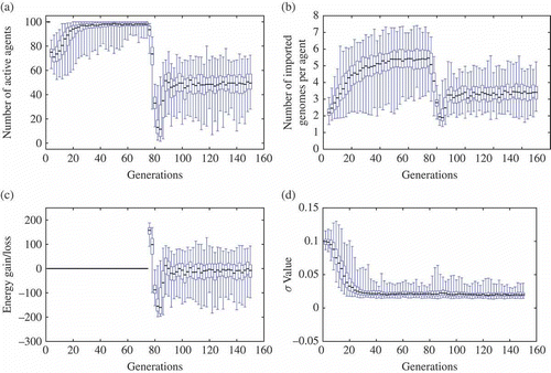
Figure 3. Experimental results for some (randomly chosen) specific runs. Note the oscillations during the ‘energy’ set-up – these oscillations are smoothed and shadowed in Figure 2 because of the large number of runs considered. (a)–(d) The number of active agents oscillates around the stable solution for mEDEA in this experiment (i.e. a larger population cannot survive in the environment, while a smaller population does not exploit all available resources. Oscillations are due to food regrowing (see text for details)).

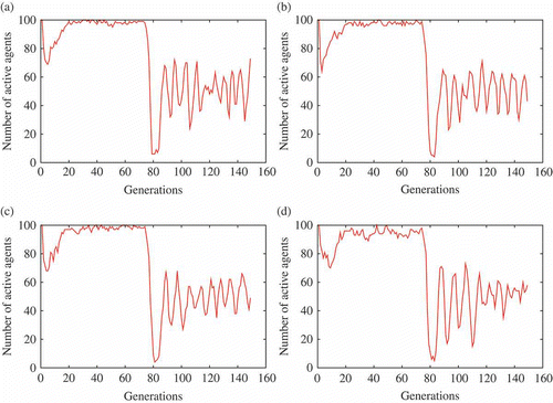
In both set-ups, all indicators rise to reach stable average values and some conclusions can be drawn: firstly, both set-ups show an increase in both mating opportunities (number of imported genomes) and survival rate (number of active agents). Secondly, switching set-ups initially lead to a drop of both indicators, followed by a quick recovery through evolutionary adaptation due to the spread of one of the few surviving, yet fit, genomes facing few competitors. This interpretation is supported by the increasing value of the energy balance which is a key element for the second set-up. It is notable that the energy balance stays around 0, which is sufficient to guarantee agent survival. This is not a surprise as maximizing harvesting may imply a cost with regard to looking for mating partners. On the other hand, the Gaussian mutation parameter is not really influenced by the change of environmental set-ups (except for a slight increase in maximum values) and remains close to its minimal value (the update scheme is biased towards small values). While the results may vary among runs, with a great difference between minimal and maximal values for each indicator, values between the upper and lower quartiles are remarkably close given the noise inherent in this kind of experiment. Indeed, complete extinctions were only observed after switching to the ‘energy’ set-up in 3 of the 100 runs (results not shown).

However, we must be very cautious with the interpretation of these results. For example, the quality of the equilibrium between maximizing mating opportunity and coping with environmental constraints (i.e. avoiding walls, avoiding collisions with other agents and harvesting) is difficult to estimate, as such an equilibrium may (and appears to) imply suboptimal values for both related indicators. In fact all interpretations provided so far rely on the assumption, that values monitored in the experiment are actually correlated with genome survival. In order to test this assumption, a new experimental set-up is defined from the results obtained so far: the post-mortem battle experiment (or battle experiment, for short). The battle experiment is loosely inspired by competitive co-evolution, where each individual competes against a hall-of-fame of the best individuals from every past generation [26], so as to estimate the fitness rank of one individual within all possible (or at least, all available) situations. For the current experiment, one ‘battle’ is achieved by randomly picking 10 generations from the same set-up and extracting one random genome from each of these generations. Then, each genome is copied into 10 different agents, resulting in 100 agents that are immersed in the same set-up they evolved in. Variation is turned off, and evolution is re-launched. After 100 generations of random selection and replacement, the number of copies of each genome is accounted for and used to compute a ‘survival score’. As an example, one genome gets a maximal score if it succeeds in taking control of all the agents. Average results over 1000 battles are given in Figure 4. In both set-ups genomes from later generations display better survival than early genomes. Moreover, battles on the second set-up show the population recovers very quickly following environmental change, possibly to stable but limited strategies as the number of active agents is far from the maximum. Also, these histograms lack the misleading artefacts observed in previous graphs regarding the early generations in both set-ups: genomes from generation 0 do not benefit anymore from uniform sampling of starting location, and genomes from generation 75 start with the same initial energy level as genomes from every other generation.

Figure 4. Genome battles on both set-ups ((a) free-ride set-up ; (b) energy set-up). Average success scores for each generation – both histograms are the results of 1000+ battles (see text for details).

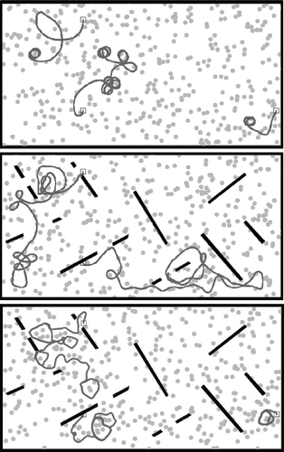
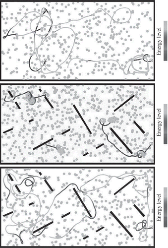
The efficiency of the algorithm is also confirmed by looking at the resulting behavioural strategies. Examples of behaviours observed in both the free-ride and energy set-ups are shown in Figures 5 and 6, resulting from agents driven by genomes obtained in the late generations of both set-ups. In the ‘free-ride’ set-up, genomes tend to lead to rather conservative behaviours, with obstacle avoidance but limited exploratory behaviour. On the other hand, genomes from the later generations of the ‘energy’ set-up show a different behavioural pattern, favouring long distance travel and some circling around. This is an efficient strategy to avoid being stuck in a depleted area. Moreover, a closer look at trajectories (including, but not limited to what is shown here) shows that agents acquired the ability to drive towards detected food items under certain conditions, such as favouring safe areas with few obstacles whenever energy levels are low.

Figure 5. Typical examples of agents' behavioural traces in the free-ride set-up. The square symbol shows the agents' starting points. Agents are tested in environments with or without walls (i.e. black bars).

Figure 6. Typical examples of agents' behavioural traces in the energy set-up. The coloured traces account for the current energy level of the agent. The square symbol shows the agents' starting points. Agents are tested in environments with or without walls.

5. Experiment #2: emergence of consensus

The results described in Section 4 showed that the mEDEA algorithm is able to perform environment-driven adaptation and provide robustness to environmental change. However, it remains unclear as to how the whole population acquires efficient behaviours and several questions remain open: does the whole population converge to one specific ‘canonical’ behaviour? If not, how different are the behaviours? Are there transient behaviours? Is it possible for two subpopulations with different behaviours to coexist (i.e. multiple stable attractors)?

This section focuses on this problem: given a population of agents, each running mEDEA, how are efficient behaviours acquired and how are they distributed across the population. In practice, we study the emergence of consensus within a simple arena, where a population of agents may choose to exploit, or not, singularities in the environment (e.g. a particular element arbitrarily located in the environment).

5.1. Problem and experimental setting: the ‘two-suns’ set-up

Figure 7 provides a snapshot of 80 agents within the arena, with a ‘sun’ located on the east side of the arena. The problem setting is closely related to the ‘free-ride’ set-up described in Section 4.1: a population of autonomous agents is placed in an empty arena, and there is no environmental constraint except the pressure to avoid obstacles and wander around mating with one another. The sun is an intangible object that provides no advantage whatsoever – that is, there is no energy in this set-up. However, each agent is provided with two additional sensory inputs giving the orientation (relative angle) and distance to the sun. Once in a while (every 50 generations), the sun changes location from east to west (and back).

Figure 7. The ‘two-suns’ set-up: a population of agents is dropped into an empty environment where a ‘sun’ is present (the circle on the left of the image). Each agent gets information about its distance and orientation with respect to the sun, but the sun itself gives no direct advantage whatsoever (e.g. no energy). Every 50 generations, the current sun disappears and another sun appears at the opposite end of the arena.

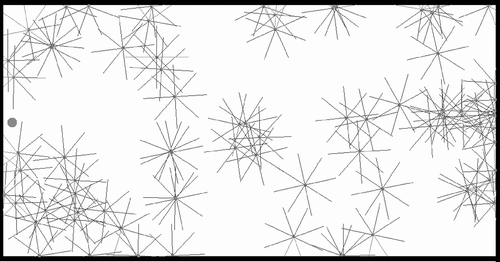
The motivation for this set-up is to provide an environment where several possible behaviours are likely to emerge and might be observed. Indeed, the sun may here be considered either a distraction and ignored or an environmental feature from which to take advantage. Our hypothesis is that in the latter case we shall be able to observe behaviours at the level of the population, with possibly one or several emergent strategies. In fact, we might expect that the sun be considered a compass and thus used as a mating location by some agents, even though there is no way for the agents to explicitly reach a consensus. Of course, offspring of a particular genome are likely to conserve a given mating strategy, resulting in a more or less widespread consensus.

In order to evaluate the emergence of consensus, two experimental parameters have been taken into account: population size and range of radio communication. Population size varies from 10 to 80 agents and radio communication takes three possible values: , (as in Section 4) and , ⁶ resulting in a total of 213 experimental settings. All experiments described in this section result from 24 independent runs for each parameter setting (i.e. a total of runs), performed on a cluster of PCs with two AMD Opteron dual-core 1.8GHz processors (AMD, Sunnyvale, CA, USA) running Ubuntu Linux. All other experimental parameters are similar to those given in Section 4.2 and the sun switches location every 50 generations (either east or west of the arena).

5.2. Results and analysis

As a general overview, Figure 8 tracks the impact of population size and radio communication settings on evolutionary adaptation. As expected, smaller populations with short radio communication distance are more prone to extinction (Figure 9). On the other hand, large populations produce a successful outcome which is independent of the communication range. Figure 10 provides much more detail at the behavioural level: each graph accounts for the final (i.e. the last step of the last generation) positions of all agents from the 24 independent runs for each population size. Both agents' final orientation and distance to the centre of the arena are plotted. Distance and orientation are given with regard to an imaginary vector at the centre of the arena (position (0,)), facing north (i.e. upwards). Distance is normalized between 0 (centre of the arena) and 100 (farthest possible location). As an example, orientation = west and distance = 80 correspond to an agent standing near, but not close to, the right border of the arena.

Figure 8. Number of successful runs (out of 24, for each population size) for different values of radio communication length: (a) , (b) ; and (c) . A run is successful whenever at least one agent is still alive at the end of the last generation. In practice, however, successful runs always feature healthy population (i.e. most agents are alive). These graphs illustrate an abrupt phase transition in the parameter space (considering population size and radio communication length) before which agents do not survive (i.e. mating becomes too difficult).

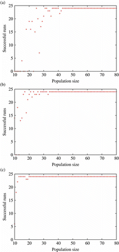
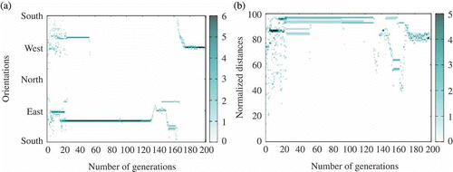
Figure 9. Example of run where the population faces extinction (extracted from one run with , ). This is but one particular example of run leading to extinction and is displayed here for illustration purpose. In this run, the agents were actually able to reach a consensus for some time. However, the relatively low population and medium communication range created a context within which a series of unsuccessful mutation (around generation 120) could not be recovered from and quickly lead to complete extinction. (a) Agents' orientation and (b) agents' distance with respect to the centre of the environment (heat map).

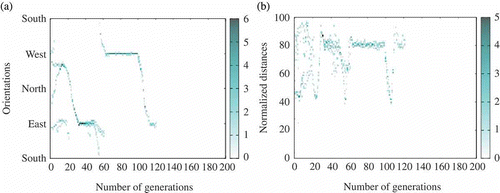
Figure 10. Tracking agents' orientation and distance to the centre of the environment for different population sizes and experimental set-ups, in the final iteration of the experiment (i.e. snapshot of the last moment of the experiment). Three different communication radii are considered. Graphs in the left column show the orientations of agents with regard to the centre of the environment. Graphs in the right column show agents' distances to the centre of the environment. The three pairs of graphs correspond, respectively, to experiments where the communication radius is set to 16 (first row), 32 (second row) and 64 (third row). For each graph, darker regions in the graphs indicate the most commonly observed orientation/distance w.r.t. the centre at the end of experiment (y-axis) for each population size parameter (x-axis) with a given communication radius value (table rows) -- this representation scheme is commonly known as a heat map. Each row is the result of aggregation of 1704 independent runs.

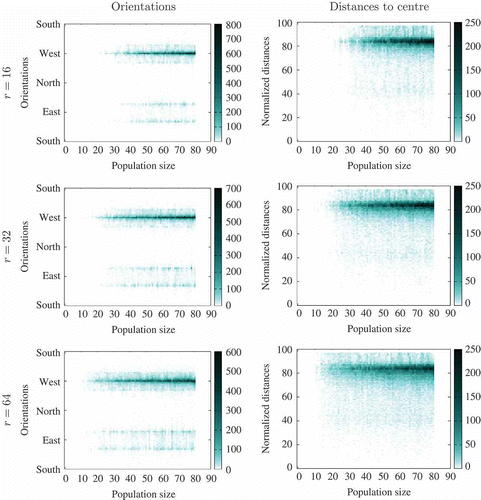
Graphs from Figure 10 illustrate that in most experiments, the vast majority of agents stand very close to the sun (west, far away from centre), and that the (few) remaining agents are located in the region of the arena opposite the sun with a preference for corners (either north–east–east or south–east–east, far away from the centre). From these graphs, we can see that at least two kinds of consensus have emerged: ‘towards sun’ (Figure 11) and ‘away from sun’ (Figure 12). However, questions remain open as to the existence of other kinds of consensus and/or the possibly simultaneous occurrence of several types of consensus. These questions were addressed by taking a closer look at the experiments from the qualitative viewpoint (i.e. hand analysis of the logs) to identify the kind of consensus (Figure 13) reached. Table 3 summarizes the results. Results shown in the table were aggregated by randomly sampling one run of each parameter setting and qualitatively evaluating the outcome of the simulation by a human expert.

Table 3. Various types of consensus

Towards sun	Away from sun	Double consensus	Misc	Extinction

Figure 11. Example of consensus towards the sun (extracted from one run with , ). Distances vary between 0 (agent in the centre of the environment) and 100 (agent in a corner). (a) Agents' orientation and (b) distance with respect to the centre of the environment (heat map).

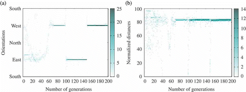
Figure 12. Example of consensus towards the side opposite to the sun (extracted from one run with , ). (a) Agents' orientation and (b) distance with respect to the centre of the environment (heat map).

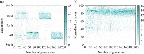
Figure 13. Example of several simultaneous consensus during one run (extracted from one run with , ). (a) Agents' orientation and (b) distance with respect to the centre of the environment (heat map).

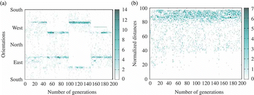
The vast majority of all runs feature at least one consensus among the agents (this was expected, as mentioned in Section 5.1). There were remarkably few runs where no clear consensus could be identified: even the ‘misc’ (Figure 14) class included either transient behaviours shifting between different consensus or different kind of stable consensus, such as following walls and ignoring the sun. Also, looking at larger population sizes (i.e. agents) results in observing an impressive 85% of the runs ending up with a unique consensus ‘towards sun’ for all agents. This tends to suggest that increasing population size introduces more stability in the evolutionary dynamics. Regarding the problem at hand, this also hints that a general agreement to go towards the Sun is an efficient consensus–which can be easily explained, as adopting this strategy is the best way for agents to meet at a precise and robust location in the environment, thus maximizing the genome's chances of survival.

Figure 14. Example of a run where agents ignore the sun, except at the very end (extracted from one run with , ). (a) Agents' orientation and (b) agents' distance with respect to the centre of the environment (heat map).

6. Testing mEDEA in a swarm of real robots

This section presents the implementation and trials of the mEDEA algorithm running on real robot hardware. It stands both as an illustration of previous results and as a methodological milestone. One of the main challenges in ER is to address the so-called reality gap [27], that is, going from simulation to the real world. However, in this article the methodological step is somewhat different as our reality gap concerns the experimental validation of the process (the mEDEA algorithm) while in traditional ER, the reality gap refers to the validation of solutions, that is, evolved control architecture with a specific behaviour, in the real world [28].

To provide experimental validation within a real robot set-up, the mEDEA algorithm has been implemented within a population of e-puck mobile robots extended with a Linux board, running at the Bristol Robotics Laboratory. In this section, the robotic environment is described, as well as considerations regarding implementing mEDEA in this context–a task which was surprisingly easy due to the nature of the algorithm. Then, results from experimental trials are described and conclusions drawn.

6.1. Technical overview

Research on swarm robotics has gained much attention in recent decades as a novel biologically inspired approach to the coordination of large groups of relatively simple robots, following simple rules [29–31]. Generally, in order to carry out real robot experiments in research laboratories, we require a robot which is small, reliable and inexpensive in order to minimize physical space and maintenance for running a relatively large number (several tens) of robots. Traditionally research laboratories have designed and built their own robot platforms for swarm robotics research, such as the Linuxbot [32], Alice [33], Jasmine [34] and Swarm-Bot [35]. There are also a number of commercially available mobile robots suitable for swarm robotics research, such as the widely used Khepera II and III from K-Team, Lego Mindstorms from the Lego company and Create from iRobot. However, the open-hardware e-puck educational mobile robot developed at the École Polytechnique Fédérale de Lausanne (EPFL) has become very popular within the swarm robotics research community within the last 3 years [36]. The e-puck combines small size -- it is about 7 cm in diameter, 6 cm tall and 660 g weight -- with a simple and hence reliable design. ⁷ Despite its small size, the e-puck is rich in sensors and in input–output devices.

The basic configuration e-puck is equipped with 8 infra-red (IR) proximity sensors, 3 microphones, 1 loudspeaker, 1 IR remote control receiver, a ring of 9 red LEDs (light-emitting diodes) + 2 green body LEDs, 1 3D accelerometer and 1 CMOS camera. Bluetooth provides the facility for wireless uploading programs and general monitoring and debugging. All sensors and motors are processed and controlled with a dsPIC30F6014A microprocessor from Microchip^TM (Microchip Technology Inc., Chandler, AZ, USA). Extension sockets provide for connecting additional sensors or actuators.

In order to ease the porting of our algorithm to real robots, we made use of the Linux board for e-puck [37]. An embedded Linux system is installed on this board as the primary operating system of the whole robot. Our algorithm is run on this board, while the lower level sensor processing and motor control is executed on the e-puck digital signal processing (DSP). One of the key advantages is the introduction of the WiFi into the system to provide fast and topologically flexible communication. This also provides a convenient way for wireless accessing and controlling the robot. In terms of productivity and ease of use, the board also allows us to use a wide range of development tools in addition to the C/ASM language development environment. The linux board for e-puck offers not only enhanced processing power, memory and communications, but a powerful control architecture for the robot. For instance, it provides flexibility in how programs may be compiled inside the robot natively (instead of cross-compiled on PC), with standard Linux tools and frameworks, including Player/Stage [38].

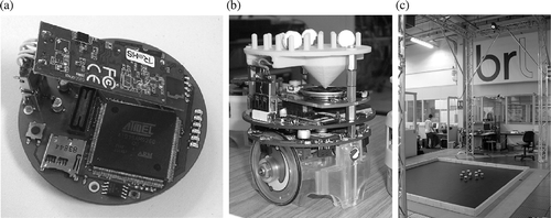
Figure 15 illustrates the modified e-puck robot and its environment. The primary function of the yellow ‘hat’ at the top of the robot is to allow us to mount reflective markers for the visual tracking system, but additionally the USB WiFi card (with its cover removed) is fitted into a slot on the underside of the hat.

Figure 15. (a) E-puck Linux extension board with USB WiFi card (casing removed). (b) An e-puck with Linux board fitted in-between the e-puck motherboard (lower) and the e-puck speaker board (upper). Also note the yellow ‘hat’ which here serves three different functions: (1) it provides a matrix of pins for the reflective spheres which allow the tracking system to identify and track each robot and (2) it provides a mounting for the USB WiFi card which slots in horizontally (the wires connecting to the WiFi card are above the USB connector). (c) Experimental swarm robotics arena with 10 Linux extended e-pucks.

Programming, initializing, starting and stopping experimental runs of a large swarm of mobile robots, then monitoring and logging data from those runs, is problematical if it has to be done manually. However, with the Linux extended e-pucks and wireless networking, we have been able to set-up a powerful infrastructure for programming, controlling and tracking swarm experiments much more conveniently. Figure 16 illustrates the overall structure of the experimental infrastructure. Each e-puck robot is configured and identified with a static IP address. They connect to the local area network (LAN) through a wireless router and can be accessed from any desktop computer connected to the network using the SSH protocol. A ‘swarm lab server’ is configured as a central code repository and data-logging pool for the swarm of robots. The server also functions as a router to bridge the swarm's wireless subnet and the local network. In addition, as there is no battery-backed real-time clock (RTC) on the extension board, the server may provide a time server for synchronization of the robots' clocks and time-stamping log data.

Figure 16. Experimental infrastructure for swarm robotics research based on the Linux extended e-puck. The swarm lab server provides a data-logging capability that combines and time stamps position-tracking data collected by the Vicon^TM system with robot status and sensor data from the e-pucks via WiFi, into a log file for post-analysis of experimental runs.

A visual tracking system from Vicon^{TM  8} (Vicon, Hampshire, UK) provides high-precision position tracking for robot experiments. This consists of four Vicon^TM MX400 cameras, one Vicon^TM MX and one HP xw6600 workstation. Each robot is uniquely identified by the visual tracking system from the pattern of reflective markers mounted on the matrix pins of the yellow hat, as shown in Figure 15(b). The tracking system is connected to the local network and broadcasts the real-time position of each tracked robot through a standard TCP/IP port. We use the position-tracking data for logging and post-analysis of experimental runs.

6.2. Implementing the two-suns experiment

In order to validate the mEDEA algorithm, an experimental setting, strongly inspired by the two-suns set-up described in Section 5, was designed. A population of up to 20 robots is placed in a empty arena. Limited-range communication is emulated using a WiFi network combined with the Vicon^TM tracking system. An additional object is introduced into the arena and is referred to as the sun: each robot in the simulation knows the sun's relative orientation and distance thanks to the Vicon^TM system. The experimenter may arbitrarily change the sun's location from time to time during the course of the experiment, switching the sun's location from one end of the arena to the other. All experiments described in this section lasted for at least 30 min, and at least 25 generations (each generation lasts appoximately. 1 min and 10 s, corresponding to 400 time steps -- this time is sufficient for a controller to cross the whole area and, therefore, meet most of the robots). The refresh rate for a robot controller is limited to five updates per second due to various technical limitations of the set-up (cf. Section 6.4).

Moreover, a set of technical issues were addressed and are listed here along with their diagnosis and solution:

•	Lack of selection pressure: ‐ diagnosis: given a small arena and few robots, it is likely that one robot can meet all other robots. This would imply that selection pressure is eliminated (see Section 2.1). ‐ solution: when the maximum number of robots is known, it is possible to limit the number of genomes that can be imported within one agent so that (with the maximum size of the genome list size and the population size). In this particular set-up, the genome list is arbitrarily limited to 17 for each robot and is filled on a first-met-first-served basis to enforce a pressure towards fast mating. Note that an extreme case would be to limit the genome list size to 1, that is, the first genome imported. However, the selection pressure would then be particularly aggressive and may not be suitable for the current experimental setting which is already prone to high variability because of the small population.
•	Slow convergence: ‐ diagnosis: because we are running physical robots in the real world, time becomes an expensive luxury. ‐ solution: the search space has been limited to a simple two-layer perceptron with no hidden layer, in contrast with previous experiments. Moreover, a large initial mutation rate is chosen. As few robots are available, large values of should promote the discovery of new solutions. Thus is set to 0.1, to 0.4 and is fixed at 0.05.
•	Risk of extinction due to small populations: ‐ diagnosis: as shown in Section 5 small populations are more prone to extinction, implying time-consuming interventions from the human supervisor. ‐ solution: a restart procedure is introduced into the algorithm. Whenever a robot stands inactive for five consecutive generations, it simply picks a new genome with random values. This simple feature thus makes it possible to avoid extinction and perhaps start from more promising regions in the search space.
•	Lack of global synchronization: ‐ diagnosis: generation count among robots cannot be synchronized on a global basis, resulting in robots with genomes from different generations. ‐ solution: the mEDEA algorithm is naturally robust to asynchronous generation count as it does not provide any survival advantage for any genome. 9

6.3. Results

An initial set of 21 experiments were conducted to explore the performance of mEDEA under various parameter settings: number of robots (from 9 to 20), generation duration, mutation values, communication radius and so on. Results from these preliminary experiments lead to several important conclusions. Firstly, the population size was found to be the most critical parameter: switching from 9 to 20 robots completely changed the observed outcome of the experiments as mEDEA clearly benefits from larger populations (cf. Section 5). Secondly, the communication radius was also identified as a key parameter: small radii (10 cm) implied versatile populations, with rare convergence towards specific behaviours while larger radii (20 cm or more) more often led to the emergence of more stable consensus within the population.

A practical conclusion is that the small number of robots available can at least be partially compensated by a larger communication radius. Indeed, experiments with a population of 20 robots and a communication radius of 10 cm would not result in more than 17 active robots at the same time while extending the radius to 20 cm regularly led to the whole population of robots being active at the same time. On the other hand, a population of 20 robots still remains relatively small with regard to experiments performed in simulation (see previous sections). A direct consequence is that in all experiments consensus were occasionally lost, switching from one kind of consensus (e.g. following the sun) to another (e.g. ignoring the sun).

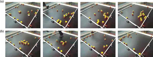
Following these preliminary experiments, eight experiments with 20 robots based on similar parameters were performed using the experimental settings described in Section 6.2. Each experiment lasted from 30 to 45 min depending on the energy consumption. The sun was moved after approximately 25 min and emergence of consensus was studied both from camera recordings and experimental data recorded using the Vicon^TM tracking system and from the internal data logs recorded by each robot. A video summarizing the main results from these experiments is publicly available. ¹⁰ A detailed analysis of the experiment shown in this video (one of the eight experiments with similar settings) is provided, using 19 robots. ¹¹ Figure 17 illustrates both the emergence of consensus to go towards the sun (Figure 17(a)) and the effect of changing the sun location (Figure 17(b)). Detailed analysis is provided both as an illustration and as an in-depth study of the internal dynamics of the algorithm during the course of the experiment.

Figure 17. Illustration from the experiment described in the text. (a) Emergence of consensus to go towards the sun. (b) Impact of changing the sun location, which shows the human changing the sun location, and convergence of the robots to the new location.

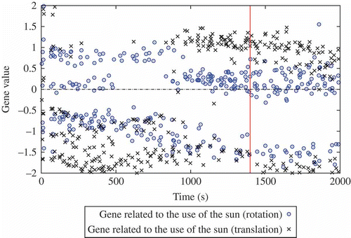
The following issues are considered: the emergence of consensus over time, the number of active robots during the run and the robustness to environment changes. Figure 18 gives the number of active robots during the course of the experiment. Figure 19 tracks the distance between each robot and the sun and is represented as a density map (or ‘heat map’, i.e. darker regions indicate the most represented distance value). Darker regions close to 0 indicate that robots stand close to the sun and are likely to be a good indication of the occurrence of sun-follower genomes in the population. Finally, Figure 20 features the weights (i.e. gene values) of the neural links connecting the sun-orientation and sun-distance sensor values to the motor rotational value of each robot (later referred to as sun-orientation gene and sun-distance gene). The weight of the sun-orientation sensor input is particularly interesting as it provides a good indication of the possible correlation between the sun's position and the robot behaviour, even though the exact nature of the correlation may be difficult to guess a priori (since motor outputs also depend on other values including sensors and NN weights).

Figure 18. Number of active robots during the course of a selected experiment. Small bars correspond to one of the robots restarting. The high bar corresponds to the sun location changing event.

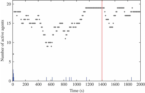
Figure 19. Distance of the robots to the sun at every time step during the course of a selected experiment. Darker regions imply more robots are located at this particular distance from the sun. The high bar corresponds to the sun location changing event.

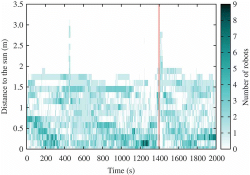
Figure 20. Tracking the values for each robot at each generation of genes related to the sun orientation: NN weights connecting the sun's orientation to agent rotational speed (sun-orientation gene) and agent translation speed (sun-distance gene). The high bar corresponds to sun location changing event.

From these data, it is possible to analyse the course of the experiment:

•	t = [0 s, 400 s] : 14–18 robots (Figure. 18) are active and a consensus to go towards the sun is emerging, while not exclusive (the dark region near 0 in Figure. 19).
•	t = [400 s, 800 s]: the consensus is suddenly lost at t = 400 s (possibly because too few robots were involved). This can be observed in both Figures. 18 and 19. The number of active robots drops to 8 and we can also observe that the genotypic signature shown in Figure. 20 does indeed change with the disappearance of sun-orientation gene values around 0.
•	t = [800 s, 1400 s]: the number of active robots increases to the maximum of 19 robots and is correlated with most robots being located near the sun (Figure. 19), possibly implying an even stronger consensus than before. Moreover, this remains stable over time until the sun's location is changed at t = 1400 s.
•	t = [1400 s, 2000 s]: Shortly after changing the sun location, the number of active robots suffers from a short decrease (to 14 robots) followed by a quick recovery (to 18 robots). This suggests good robustness in the population, an inference which is reinforced by looking at the two other figures: the robots slowly converge back to the sun and the genotypic signature remains unchanged. We can also observe that sun-follower genomes are likely to be correlated with sun-orientation gene values close to 0 (but positive).

The seven other experiments with similar settings provided comparable results. All the runs displayed the emergence of various types of consensus as well as occasional time periods in which no consensus could be identified. Also, changing the sun location had an important impact during experiments, with the vast majority of robots adopting the same ‘towards sun’ consensus. This can be explained by the fact that sun-follower genomes spread while their robot hosts were moving towards the sun. The following general conclusions can be drawn from these experiments:

•	The robot restart procedure is mostly used in the initial generations, which implies the population becomes self-sustaining (i.e. there are enough encounters between robots to avoid requiring the restart procedure).
•	The largest number of simultaneously active robots was obtained with a population of sun-followers (from 15 to 19 active robots having reached a consensus to go towards the sun).
•	Changing the sun location had different effects depending on the existence (or non-existence) of consensus in a population. Populations of robots ignoring the sun did not suffer from such a change, while sun-follower populations first suffered (i.e. some agents are lost and stop) from the sun changing location followed by a quick recovery.

6.4. Discussion of the reality gap

Implementation and trials of the mEDEA algorithm within a population of robots reveals a number of technical issues unfamiliar to experiments in simulation. Together, they comprise the reality gap between simulation and real-world experiments [27]. These issues are articulated as follows:

•	Proximity sensors are unreliable: the low quality of the IR sensors makes it very difficult to detect obstacles and/or other robots (with a binary positive response only for distances less than 1 cm). Also the e-puck body is more or less transparent, making it almost invisible in some cases. Adding a coloured plastic skirt to the robots only partly solves the problem as the proximity sensors are occasionally blinded by the skirt. As a consequence, the proximity sensors can be disregarded because of their unreliability.
•	Colliding robots are regularly unable to send/receive genomes to their neighbours. This is due to our particular set-up where local communication is emulated using the ViconTM system for computing the local communication network based on the distance between robots. While this approach was originally motivated by the lack of local robot–robot communication, it ended up as quite a problem as robots could not participate in the evolutionary adaptation process during collisions. In practice, robots were occasionally lost from the emulated communication network but always recovered when moving away from one another.
•	On-board processing is slow: the combination of on-board computation with limited hardware and the particular set-up for emulating local communication has a negative impact on the speed of execution. In fact five updates per second were observed, with often asynchronous updates of sun distance and orientation from the tracking system (i.e. out-of-date information).

Two conclusions can be drawn from these issues: Firstly, simulation and real-world experiments do differ, as expected. Secondly, however, results from the experiments showed that mEDEA is remarkably robust to the reality gap, as it manages to deal with all the issues outlined above and still demonstrates interesting behaviour that manages to survive in the environment. As a matter of fact, the most critical issue from these experiments in the real world is the small population size, whose importance was already discussed in Section 5 as it impacts the stability of the algorithm (larger populations display more stable behaviours). In the present context, the negative effect of a small population was counterbalanced by adding a restart mechanism and relying on a large enough communication range (i.e. 15–20 cm).

7. Conclusions and perspectives

This article has explored the viability of EDEA in a population of autonomous agents. We have presented the mEDEA algorithm, a particular flavour of EE, tailored to address evolutionary adaptation with implicit fitness. The mEDEA algorithm has been evaluated and demonstrated to be (1) efficient with regard to providing distributed evolutionary adaptation in unknown environments and (2) robust to unpredicted changes in the environment. We have also studied the emergence of consensus within an evolving population of agents. Large populations were shown to converge to stable, mostly unique, behavioural strategies, while smaller populations, that is, facing similar environmental conditions with fewer resources, occasionally displayed dissimilar strategies coexisting at the same time.

The mEDEA algorithm is lightweight and may be considered suitable for implementation within hardware/software set-ups with limited computation such as robotic agents. Indeed, experiments with real robots have illustrated the applicability of the algorithm to hardware implementation and displayed remarkably good behaviour in far from ideal experimental conditions (as one would expect from real robots).

Many future perspectives may be considered from this point onwards and some are already under investigation. In particular, surviving in aggressive environments requires more complex behavioural patterns, such as self-organization and coordination. Secondly, and sharing similar concerns, previous work in collective intelligence and reinforcement learning have already stressed the issue of the price-of-anarchy [39], that is, the cost of efficient selfish behaviour with regard to global population welfare. Then again, solving this issue remains an open problem especially if there is no explicit objective function to decompose. Thirdly, the work presented here targets and is limited to providing reliable survival strategies. However, our motivating claim is that one should first aim at a reliable, surviving population before then considering optimization against a predefined objective function. Within ER similar ideas have been defended in recent years: goal-oriented optimization is often better served by objectives that are loosely related to the goal (e.g. maximizing diversity [40]), while objective functions with an extensive goal description often lead to deceiving fitness landscapes and poor results. From this perspective, the research reported in this article can be seen as addressing the first part of the trade-off between achieving survival (i.e. maintaining communication among the population) and optimizing goal-oriented behaviours (as specified by the supervisor before runtime).

Acknowledgement

This work was made possible by the European Union FET Proactive Intiative: Pervasive Adaptation funding the Symbrion project under grant agreement 216342.

Notes

1. With the notable exception of works in the field of artificial life [17–21]. However, that research area strongly differs in its core motivation to the work presented here as we ultimately aim towards engineering solutions.

2. 11 input neurons; 5 hidden neurons; 2 output neurons; 1 bias neuron. The bias neuron value is fixed to 1.0 and projects onto all hidden and output neurons.

3. Note that the simulation begins with each agent containing a randomly initialized genome.

4. Combining the regrow delay update scheme with the equation relating the required number of food items and population size leads to a quadratic equation with one positive solution. In this set-up, the optimal population size is strictly below 80 agents. However, this set-up is very aggressive as soon as 50+ agents are active.

5. Evolutionary Robotics Database: http://www.isir.fr/evorob db/.

6. As a reminder, proximity sensor length is 64 (cf. snapshot in Figure 7 for interpretation).

7. The open-hardware design can be found at http://www.e-puck.org.

8. http://www.vicon.com.

9. As a counter example, generation times do need to be equal across robots as longer generation times would lead to more opportunities for a genome to spread.

10. http://www.youtube.com/watch?v=_ilRGcJN2nA (Accessed 1 December 2010).

11. One robot was removed due to technical failure in a previous experiment.

References

- Bonabeau , E. , Dorigo , M. and Theraulaz , G. 1999 . Swarm Intelligence: From Natural to Artificial Systems , Oxford : Oxford University Press .
- Trianni , V. , Nolfi , S. and Dorigo , M. 2008 . “ Evolution, self-organization and swarm robotics ” . In Swarm Intelligence, Natural Computing Series , Edited by: Blum , C. and Merkle , D. 163 – 191 . Berlin : Springer .
- Baele , G. , Bredeche , N. , Haasdijk , E. , Maere , S. , Michiels , N. , Van de Peer , Y. , Schmickl , T. , Schwarzer , C. and Thenius , R. 2009 . Open-ended on-board evolutionary robotics for robot swarms , 1123 – 1130 . Trondheim , , Norway : Proceedings of the IEEE Conference on Evolutionary Computation (CEC 2009) .
- Bernstein , D.S. , Givan , R. , Immerman , N. and Zilberstein , S. 2002 . The complexity of decentralized control of Markov decision processes . Math. Oper. Res. , 27 ( 4 ) : 819 – 840 .
- Kohl , N. and Stone , P. 2004 . Policy gradient reinforcement learning for fast quadrupedal locomotion , 2619 – 2624 . New Orleans , LA : Proceedings of the IEEE International Conference on Robotics and Automation .
- Marbach , P. and Tsitsiklis , J.N. 2003 . Approximate gradient methods in policy space optimization of Markov reward processes . J. Discrete Event Dyn. Syst. , 13 : 111 – 148 .
- Williams , R.J. 1992 . Simple statistical gradient-following algorithms for connectionist reinforcement learning . Mach. Learn. , 8 : 229 – 256 .
- Taylor , M. , Whiteson , S. and Stone , P. 2006 . Comparing evolutionary and temporal difference methods for reinforcement learning , 1321 – 1328 . Seattle , WA : Proceedings of the Genetic and Evolutionary Computation Conference (GECCO) .
- Taylor , M.E. , Whiteson , S. and Stone , P. 2007 . Temporal difference and policy search methods for reinforcement learning: An empirical comparison , 1675 – 1678 . Vancouver , , Canada : Proceedings of the Twenty-Second Conference on Artificial Intelligence (AAAI-07) .
- Ficici , S. , Watson , R. and Pollack , J. 1999 . Embodied evolution: A response to challenges in evolutionary robotics , Edited by: Wyatt , J.L. and Demiris , J. 14 – 22 . Lausanne , , Switzerland : Proceedings of the Eighth European Workshop on Learning Robots .
- Elfwing , S. , Uchibe , E. , Doya , K. and Christensen , H.I. 2005 . Biologically inspired embodied evolution of survival . Proceedings of the 2005 IEEE Congress on Evolutionary Computation IEEE Congress on Evolutionary Computation . September 2–5 2005 , Edinburgh , UK. Edited by: Corne , D. , Michalewicz , Z. , Dorigo , M. , Eiben , G. , Fogel , D. , Fonseca , C. , Greenwood , G. , Chen , T.K. , Raidl , G. , Zalzala , A. , Lucas , S. , Paechter , B. , Willies , J. , Merelo , J.J. Guervos , Eberbach , E. , McKay , B. , Channon , A. , Tiwari , A. , Volkert , L. Gwenn , Ashlock , D. and Schoenauer , M. Vol. 3 , pp. 2210 – 2216 . UK : IEEE Press .
- Usui , Y. and Arita , T. 2003 . Situated and embodied evolution in collective evolutionary robotics , 212 – 215 . Oita , , Japan : Proceedings of the 8th International Symposium on Artificial Life and Robotics .
- Watson , R.A. , Ficici , S.G. and Pollack , J.B. 2002 . Embodied evolution: Distributing an evolutionary algorithm in a population of robots . Rob. Auton. Syst. , 39 ( 1 ) : 1 – 18 .
- Wischmann , S. , Stamm , K. and örgötter , F. W . 2007 . “ Embodied evolution and learning: The neglected timing of maturation ” . In Advances in Artificial Life: 9th European Conference on Artificial Life , Edited by: Francesco , Almeida e Costa . Vol. 4648 , 284 – 293 . Lisbon , , Portugal : of Lecture Notes in Artificial Intelligence, Springer-Verlag .
- Bredeche , N. , Haasdijk , E. and Eiben , A.E. 2009 . On-line, on-board evolution of robot controllers , 110 – 121 . Proceedings of Artificial Evolution/Evolution Artificielle (EA'09), Strasbourg, France .
- Montanier , J.-M. and Bredeche , N. 2011 . “ Embedded evolutionary robotics: The (1 + 1)-restart-online adaptation algorithm ” . In New Horizons in Evolutionary Robotics: Extended Contributions from the 2009 EvoDeRob Workshop , Edited by: Doncieux , S. , Bredeche , N. and Mouret , J.-B. 155 – 168 . Berlin : Springer .
- Bedau , M.A. 2001 . Comparison of the growth of adaptive structure in artificial life models and in the fossil record . PaleoBios , 21 : 30
- Bedau , M.A. , McCaskill , J.S. , Packard , N.H. , Rasmussen , S. , Adami , C. , Green , D.G. , Ikegami , T. , Kaneko , K. and Ray , T.S. 2000 . Open problems in artificial life . Artif. Life , 6 : 363 – 376 .
- Holland , J.H. 1994 . “ Echoing emergence: Objectives, rough definitions, and speculations for echo – class models ” . In Complexity: Metaphors, Models and Reality , Edited by: Cowan , G.A. , Pines , D. and Meltzer , D. 309 – 342 . Reading , MA : Addison-Wesley .
- Ray , T. 1991 . Is it alive, or is it GA? , San Diego , CA : Proceedings of International Conference on Genetic Algorithms .
- Spector , L. , Klein , J. , Perry , C. and Feinstein , M. 2005 . Emergence of collective behavior in evolving populations of flying agents . Genet. Program. Evolvable Mach. , 6 ( 1 ) : 111 – 125 .
- Dawkins , R. 1976 . The Selfish Gene , Oxford : Oxford University Press .
- Fletcher , J.A. , Bedau , M.A. and Zwick , M. 1998 . “ Effect of environmental structure on evolutionary adaptation ” . In Artificial Life VI , Edited by: Adami , C. , Belew , R. , Kitano , H. and Taylor , C. 189 – 198 . Cambridge , MA : MIT Press .
- Beyer , H.-G. and Schwefel , H.-P. 2002 . Evolution strategies – a comprehensive introduction . Nat. Comput. , 1 : 3 – 52 .
- Futuyma , D. 2009 . Evolution , 2nd , Sunderland , MA : Sinauer Associates Inc .
- Rosin , C. and Belew , R. 1996 . New methods for competitive coevolution . Evol. Comput. , 5 : 1 – 29 .
- Jakobi , N. , Husband , P. and Harvey , I. 1995 . “ Noise and the reality gap: The use of simulation in evolutionary robotics ” . In Advances in Artificial Life: Proceedings of the Third European Conference on Artificial Life , Edited by: Moran , F. , Moreno , A. , Merelo , J. and Chancon , P. 704 – 720 . Berlin : Springer-Verlag .
- Nolfi , S. and Floreano , D. 2000 . Evolutionary Robotics: The Biology, Intelligence, and Technology of Self-Organizing Machines , Cambridge , MA : MIT Press/Bradford Books .
- Şahin , E. and Spears , W. 2005 . Swarm Robotics Workshop: State-of-the-Art Survey , Vol. 3342 , New York : of Lecture Notes in Computer Science, Springer .
- Şahin , E. and Winfield , A.F.T. 2008 . Swarm Intelligence: Special Issue on Swarm Robotics , Vol. 2 , Berlin : Springer .
- Dorigo , M. and Şahin , E. 2004 . Autonomous Robots: Special Issue on Swarm Robotics , Vol. 17 , Berlin : Springer .
- Winfield , A.F.T. and Holland , O.E. 2000 . The application of wireless local area network technology to the control of mobile robots . Microprocess. Microsyst. , 23 ( 10 ) : 597 – 607 .
- Caprari , G. , Estier , T. and Siegwart , R. 2002 . Fascination of down scaling – Alice the sugar cube robot . J. Micro Mechatron. , 1 ( 3 ) : 177 – 189 .
- Kornienko , S. , Kornienko , O. and Levi , P. 2005 . Collective AI: Context Awareness via Communication , 1464 – 1470 . San Francisco , CA : IJCAI'05: Proceedings of the 19th International Joint Conference on Artificial Intelligence, Morgan Kaufmann Publishers Inc .
- Gross , R. , Bonani , M. , Mondada , F. and Dorigo , M. 2006 . Autonomous selfassembly in swarm-bots . IEEE Trans. Rob. , 22 ( 6 ) : 1115 – 1130 .
- Mondada , F. , Bonani , M. , Raemy , X. , Pugh , J. , Cianci , C. , Klaptocz , A. , Magnenat , S. , Zufferey , J.-C. , Floreano , D. and Martinoli , A. 2009 . The e-puck, a robot designed for education in engineering , Vol. 1 , 59 – 65 . Castelo Branco , , Portugal : Proceedings of the 9th Conference on Autonomous Robot Systems and Competitions .
- Liu , W. and Winfield , A.F.T. 2011 . Open-hardware e-puck Linux extension board for experimental swarm robotics research . Microprocess. Microsyst. , 35 ( 1 ) : 60 – 67 .
- Vaughan , R. 2008 . Massively multi-robot simulation in stage . Swarm Intell. , 2 ( 2–4 ) : 189 – 208 .
- Wolpert , D.H. and Tumer , K. 2001 . Optimal payoff functions for members of collectives . Adv. Complex Syst. , 4 ( 2/3 ) : 265 – 279 .
- Lehman , J. and Stanley , K.O. 2011 . Abandoning objectives: Evolution through the search for novelty alone . Evol. Comput. , 19 ( 2 ) : 189 – 223 .