Fast and save container cranes as bilevel optimal control problems

Abstract

For the use of container cranes in high rack warehouses, reference trajectories can be obtained from optimal control problems in order to control the swinging of the crane system during the fast movement and in order to reach an equilibrium position at the end of the trajectory. Safety requirements extend these problems to bilevel optimal control problems, where the existence of alternative stop trajectories has to be guaranteed. A method as to how these complex problems can be reduced to conventional optimal control problems, even under control and state constraints, is presented together with numerical examples.

Keywords:

• bilevel optimal control
• crane system
• hybrid method

1. Introduction

A successful cooperation between engineers and mathematicians led to the realization of a new concept of storage techniques despite the difficulty of placing new products on the market of warehouse logistics. To satisfy the high standards for availability, the planning of new high rack warehouses will be easier, if the necessary investments can be done in proven systems instead of recently introduced ones.

The engineers constructed a crane system to allow loading and unloading processes in a warehouse rack without touching the ground. Providing optimal reference trajectories to operate the crane system was an easy task for the mathematicians. However, during the cooperation further requirements for the path planning arose: The goals from the engineering point of view aligned with the possibilities of mathematics so well that a software library could be developed for an industrial usage of the crane system. Currently, this solution is sold by Westfalia Holding GmbH & Co. KG under the name Aviator.

Due to industrial standards, a special safety requirement for the trajectory of the crane system had to be considered. This led us to the formulation of bilevel optimal control problems and the necessity of solving them.

The attribute bilevel generally describes the interaction of two decision makers or players actuating hierarchically on different sets of free variables. The first formulation of this concept dates back to 1934, when von Stackelberg [1] described a market situation consisting of two vendors. One of them is the market leader and therefore decides first, knowing all possible reactions of his rival. This means also that the profit of the leader only depends on his own decisions.

For static systems, bilevel programming problems extend problem formulations of linear and nonlinear programming (NLP) to two players, where the first player – the leader – knows in advance how the second player – the follower – will react to his decision. Bracken and McGill [2] introduced this class of problems as NLP problems with constraints as the solution of another NLP problem. Dempe collects various theoretical results in [3], and Bard presents practical solution methods in [4].

For dynamic systems, Chen and Cruz are the first to combine two conventional optimal control problems to a bilevel optimal control problem in [5]. A more detailed description together with theoretical results is given by Ye [6].

The solution of an optimal control problem minimizes the dynamic behaviour of a system with respect to an objective function. Current problem formulations of bilevel optimal control problems only consider dynamical behaviour within each of both optimal control problems involved. The industrial application made it also necessary to add the dynamic component in the way in which these two problems are coupled [7].

However, a similar problem was introduced by Mayrhofer and Sachs [8] for emergency trajectories of a hypersonic flight system and was solved using a parametric optimization method.

2. Container cranes in high rack warehouses

Commercial buildings more than 12 m high for automated storage of goods are named high rack warehouses. They can directly be linked to manufacturing plants or just serve for stock turnover. Even if each industrial sector stocks different types of goods, a warehouse generally is used for goods of a similar type.

The storage area as the main part of a warehouse is filled with parallel installed shelf units providing space for thousands of pallets. Between two shelves a lane is kept free to access these storing positions.

The automated logistic decision, where to store each good, is made by warehouse management systems. The transport of the goods in the lane is mostly automated too. The conventional solution consists of a floor-driven shelf access equipment, which moves along rails along the lane and lifts the payload to the designated height of the storing position, similar to a fork lift truck. An advanced trajectory planning is not necessary for this kind of transport unit, as it behaves like a rigid single body system, if appropriate upper limiting values for accelerations and velocities are specified.

A ceiling-driven container crane can be used to fulfil the same tasks. It has to be treated as a multibody system, as the two main tasks positioning and load pick up are distributed to these modules, which are connected via cable ropes:

	Trolley. A trolley is used for positioning the payload. For horizontal movement, the trolley rides along rails on the top of the warehouse rack, similar to a trolley on a crane arm. For vertical movement, a set of rope drums on the trolley is used to lower or lift a load-carrying equipment.
	Load-carrying equipment. After the load-carrying equipment is anchored at the correct storing position, it can put or pick the payload by accessing the shelf with a fork-like construction.

As soon as the trolley starts moving, the load-carrying equipment will start to swing. When the trolley reaches its terminal position, the load-carrying equipment will continue swinging, and an access to the shelf is impossible. Using a feedback control law to damp the swinging at the terminal position would need too much time. An attempt to use a feedback control law to keep the load-carrying equipment right below the trolley already during the movement of the crane system failed. As soon as the trolley changed its position, the relative displacement between the two rigid bodies was cleared by returning the trolley to its original position.

To operate the crane system in the shelf units, it is fundamental to allow for these displacements. This requires a path planning for the crane system, which is able to position the load-carrying equipment at any storing position without any residual oscillations and with a precision of ±1 cm. A typical data set for the dimensioning of a crane system is provided in Table 1.

Table 1. Parameters for a typical crane system

Length of lane	40–80 m
Height of shelf	5–16 m
Maximum payload	5 t
Maximum horizontal velocity	3 m/s
Maximum vertical velocity	1.5 m/s
Maximum horizontal acceleration	1 m/s^2
Maximum vertical acceleration	1 m/s^2

2.1 Mathematical model of a crane system

For the path-planning problem, the dynamical behaviour of the oscillating multi-body system has to be modelled. We assume a mathematical pendulum, that is the mass m of the load-carrying equipment is concentrated in one point, and the cable ropes are massless. Gravity is the only force acting in the system, F_G  = m · g, where g = 9.81 m/s² is the local acceleration due to gravity. Depending on the current amplitude φ, the restoring force brings the mass back to the equilibrium position by accelerating it, see Figure 1(a). For simplicity, we assume this force to act horizontally and not along the circular arc. Omitting all frictional forces, the horizontal position r of the mass holds:

(1)

Figure 1. Model of the crane system. (a) Fixed length of cable rope, (b) Variable length of cable rope.

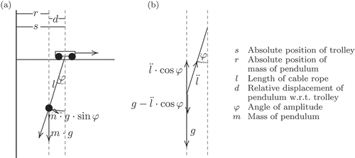
Denoting the relative displacement of the mass with respect to the pivot by d, and the length of the rope by l, we get . The horizontal position s of the pivot, which is attached to the moving trolley, holds s = r + d. Applying the second derivative to (1) yields If the length of the rope l is variable, g has to be replaced by the effective acceleration or for small angles φ, see Figure 1(b). This leads to the model of the crane system

(2)

which is independent from the system's masses.

2.2 Advantages and disadvantages

Our industrial partner advertises several advantages of its product:

	Automation. For a later automation of existing manually operated warehouses, only few changes have to be made to the shelves.
	Expandability. To increase the performance of the warehouse, more crane systems can operate in one lane. Some strategies for collision avoidance between these crane systems are detailed in [7].
	Flexibility. Due to lack of space, it might be necessary to spare areas of the shelf units for passages perpendicular to the shelves. To bypass these obstacles, the trolley has to lift the load-carrying equipment to the necessary height. Even shelves with uneven bases can be operated smoothly from the top.
	Reduced costs. Compared with conventional shelf access equipments, the crane systems need less material. Instead of robust constructions of steel to reach large heights, the trolley can use cable ropes to access large depths. As less material has to be moved during the transport of the payload, energy costs are on the decrease as well.

For the continuous use in an industrial high rack warehouse, the crane system has to satisfy different safety requirements, which have to be considered during path planning.

	Collision avoidance. Neither the trolley nor the load-carrying equipment are allowed to go beyond the extent of the shelf unit. Possible obstacles like passages have to be avoided.
	Emergency stop. In the case of a system failure or a power outage, the movement of the trolley will be stopped by mechanical brakes. As the load-carrying equipment is expected to start swinging intensely during this braking, the path planning might reduce maximum velocities in critical areas.
	Safety stop. At any time during the tracking of a planned trajectory, the user should have the ability to invoke a controlled braking, so that the whole system comes to rest without any oscillation within a given time. The final positions of the trolley and the load-carrying equipment are free, but have to be admissible. To ensure that this safety stop is possible, an appropriate set of alternative trajectories has to be uploaded to the control unit before starting to track the main trajectory.

The requirement for the safety stop leads to this bilevel problem: On the one hand, each starting point of a safety stop trajectory depends on the main trajectory. One the other hand, for any state of the main trajectory, it must be possible to switch to an alternative safety stop trajectory, which means that the main trajectory depends on the safety stop trajectories as well. Hence neither the main trajectory nor the alternative trajectories can be found separately.

3. Optimal control

Path planning of trajectories for the crane system in a warehouse is a standard problem of optimal control. Generally, in optimal control problems, a control function has to be determined in order to manipulate a state function over a period of time t_f . denotes the class of j times piecewise continuously differentiable and j – 1 times continuously differentiable functions from an interval to . The system dynamics for the state x is described by a system of first-order differential equations

with continuously differentiable with respect to x and u. The components of the initial state and the final state can be set partially or completely by the equation with a continuously differentiable function . Constraints for the control u(t) and the state x(t) can be postulated as inequality conditions for with continuously differentiable. The solution of the optimal control problem is a pair of optimal trajectory and optimal control u*(t), which minimizes the objective function

over all admissible solutions with and , continuously differentiable.

The standard problem of optimal control reads as follows:

(3)

Additionally, a set of free variables can also be considered as an optimization parameter. For example, the process time t_f can be unknown.

Two categories of methods have been developed to treat problems of type (3). Our strategy to solve bilevel optimal control problems in Section 4 can be seen as a combination of both categories.

3.1 Indirect methods

Indirect methods need a deep insight into the theory of optimal control, as it is given in Bryson and Ho [9] and Ioffe and Tihomirov [10]. The indirect methods convert (3) into a boundary value problem using the necessary conditions from Theorem 3.1 to eliminate the unknown control u(t) from the problem.

In the unconstrained version of (3), the inequality for the constraints is omitted and only box constraints for the control might be considered in the form , for all . For this special case, which will be needed in Section 4, the Hamiltonian is defined as

with a parameter and the adjoints . The minimum principle of Pontryagin [11] states as follows:

Theorem 3.1:

Let be a solution of the unconstrained problem (3). Then there exist , , not all vanishing, so that these equations hold:

	Minimum condition. (4)
	Adjoint differential equations. (5)
	Transversality conditions. (6)

The Hamiltonian is said to be regular with respect to an optimal solution , if there exists ϵ > 0, so that the function has a unique minimizer

for all with In this case, the optimal control is the unique function . For for a neighbourhood of , can be calculated from

Similar results for the constrained case exist; see Neustadt [12] for a mixed constraint and Maurer [13] for state constraints. General results are yet to be proven, see Hartl et al. [14].

3.2 Direct methods

By discretizing the control and state functions, direct methods approximate the infinite dimensional optimal control problem by an NLP problem with a finite number of parameters.

The continuous time axis is replaced by a set of discrete grid points , and from the control function u(t) in (3) only a vector of discrete values with remains. Intermediate values of u(t) can be retrieved by linear interpolation, if needed:

The state function x(t) is also reduced to discrete values . If the Euler method is used to integrate the integral and the system of differential equations in (3), it can be approximated by

To reduce the problem size even more, only the discretized control values have to be stored, as the discretized states xⁱ can be calculated using the control values and the initial values x ₀:

Finally, the optimal control problem reduces to the standard NLP problem

The software library NUDOCCCS by Büskens [15] has also implemented higher order methods to transcribe optimal control problems into NLP problems to solve them with a sequential quadratic programming (SQP) method.

3.3 Parametric sensitivity analysis

Understanding how an optimal solution changes with respect to small perturbations of the perturbed optimal control problem

(7)

helps to evaluate the quality of the solution. An implementation of a sensitivity analysis for optimal control problems is proposed by Büskens [16]. For a fixed value p = p ₀, the solution is called the reference or nominal solution. For simplicity and without loss of generality, f ₀ ≡ 0 is assumed here.

Using direct methods, sensitivity derivatives with respect to p for the functions and variables of (7) can be formulated, if the optimal solution is differentiable with respect to the perturbation parameters, see Büskens and Maurer [17]. This is the case for scalar-valued control functions under scalar-valued mixed constraints, see Maurer and Pesch [18,19], or vector-valued control functions under mixed constraints, see Malanowski and Maurer [20,21]. A general proof for all types of optimal control problems is still missing.

The results of Fiacco [22] and Büskens and Maurer [23] for parametric sensitivity analysis of NLP problems can be transferred to the discretized version of (7),

(8)

where the active inequalities for g and the boundary conditions for ω are combined to the equations for . For , the discretized control uⁱ (p) depends on the perturbation parameter p, and the state xⁱ (u, p) can be integrated using u^j (p), .

The Lagrangian for this NLP problem is

with Lagrange multipliers . The sensitivity derivatives for the discretized control variables are given by calculating the sensitivity derivatives for the optimization parameters of the NLP problem (8)

(9)

with the abbreviations , . For , the sensitivity derivative can be calculated using the chain rule as

(10)

These derivatives can be used for a real-time approximation of the perturbed optimal control problem

(11)

The general result is that the optimal solution depends continuously on locally perturbed parameters, for example, the initial values.

4. Bilevel optimal control

In an optimal control problem, a control function has to be determined in order to minimize an objective function . If another person is allowed to interfere in the system using a new control function , he will try to follow his own goals . This becomes a bilevel optimal control problem if the first player knows the possible reactions Ψ(u) of the second player in advance:

(12)

The leader's selection of a control function u(t) is only feasible if the follower is able to generate a non-empty set of optimal solutions Ψ(u).

Following the formulation of Ye [6], the state function is assigned to the lower level and is determined by the system dynamics . Both players have to make sure that the boundary condition holds.

As for most mechanical applications boundary values for y are either explicitly given or free, only boundary conditions of type

(13)

will be considered here. The index set determines if y_i (0) is fixed for i ε R ₀. Similarly determines if y_i (t_f ) is fixed for .

4.1 Optimistic solution

The bilevel optimal control problem stated in Section 6 for the crane system generates one trajectory in the leader's problem and a set of stopping maneuvres in the follower's problem. As these paths are coordinated centrally from one control unit, it makes sense to assume a cooperative behaviour of the follower in case of doubt. If the solution Ψ(u) is not unique, the leader may pick that element, which minimizes his objective function:

4.2 Reduction to single-level problem

The necessary optimality conditions of Theorem 3.1 can be used to determine solution candidates for the lower level problem. In general, the solution should be confirmed using sufficient conditions. However, if the lower level problem is convex, the necessary conditions are already sufficient, and the lower level problem can be replaced by its necessary optimality conditions. The resulting single-level optimal control problem can be solved with direct methods.

The Hamiltonian of the lower level problem in (12) for a fixed control u of the upper level problem is needed for the optimality conditions:

Using Theorem 3.1, the adjoint variables λ(t) have to satisfy the adjoint differential equations

for an optimal solution of the lower level problem. Several assumptions have to be fulfilled in order to reduce the bilevel optimal control problem (12) to an optimal control problem:

i.	The Hamiltonian h is regular with respect to an optimal solution . In this case, the control v is determined by (14)
ii.	Equation (14)(14) can be solved analytically for in order to eliminate the control v from the control problem. Otherwise Equation (14)(14) would have to be considered an equality constraint.
iii.	The case λ0 = 0 can be excluded, so that λ0 can be set to 1.
iv.	The lower level problem of (12) is convex.

For boundary conditions (13), the bilevel optimal control problem reduces to

(15)

This optimal control problem can be transcribed into an NLP problem, and due to the structure of the Hessian and the Jacobian, sparse SQP solvers would minimize calculation times. In some cases it can still be solved analytically, cf. [7] for an example.

If the follower's scope of action is reduced, the leader's goals can be reached more easily. In the bilevel optimal control problem (12), each component v_i (t) of the control of the lower level is now constrained by

(16)

After calculating from Equation (14)(14), these values have to be limited to (16) before v is eliminated from the problem:

(17)

Theorem 3.1 assures that the assembled control function is optimal.

Unlike control constraints, state constraints can cause discontinuities in the adjoints λ(t). In addition to the adaption of the control function on state-constrained intervals, jump conditions for the adjoints would have to be formulated.

In Section 6.2, an alternative solution is proposed to handle state constraints suboptimally.

4.3 Separation of system dynamics

To keep the dimension of the adjoint differential equation system small in (15), conditions are formulated under which components of the state y(t) of (12) can be moved from the lower level problem to the upper level problem.

For this, an additional state function is added to the lower level problem, using . For simplicity, the formulation given here is restricted to known initial values x(0) and y(0):

(18)

with Ψ(u) set of solutions of

The Hamiltonian for the lower level problem yields

The functions ν(t) and λ(t) denote the adjoint variables to x(t) and y(t), respectively. The adjoint differential equations are

and the control can be calculated via , that is

(19)

if the case λ₀ = 0 is excluded again. This reduces (18) to

(20)

Alternatively, the new state variable x(t) could be added to the upper level problem:

(21)

with Ψ (x, u) set of solutions of

The Hamiltonian for the lower level problem would be

and the adjoint differential equation system would consist of

For λ₀ ≠ 0, the control would be gathered from

(22)

and (21) would reduce to

(23)

To formulate sufficient conditions, under which the reduced systems (20) and (23) coincide, the control v(t) has to be calculated equally using (19) and (22). If does not depend on v(t), and (19) can be solved for independent of ν(t).

For a congruence of the adjoint differential equations for λ(t) in (20) and (23), is required. The adjoint ν(t) will be used neither for the evaluation of the objective function F ₀ nor for the differential equations for x(t), y(t) or λ(t) and can be omitted.

These results are summarized in the following theorem:

Theorem 4.1:

The differential equation system

with initial value x(0) = x ₀ can be attached to the upper as well as the lower level problem. The optimal solutions remain unaffected.

A similar result can be shown for the system . In general, the optimal solutions may change if is attached to the lower or the upper level problem, see [7] for a counterexample.

Naturally, if two distinct systems are used in the upper and the lower level of the bilevel optimal control problem, the assumption of Theorem 4.1 holds. The lower level system can also operate on a particular time scale .

5. Time dependent coupling

In Section 4, the complete state information of the upper level was transferred to the lower level. To emulate the alternative ending scenario for a safety stop at a given time as proposed in Section 2, the state ξ = x(ϑ) of the leader's system can be passed to the follower to generate a solution set Ψ(ξ), see also Figure 2.

(24)

with fixedand Ψ(ξ) set of solutions of

Figure 2. Single, continuous and discrete time dependent coupling between upper level (axis from 0 to 12s) and lower level (axis from 0 to 4s) problem.

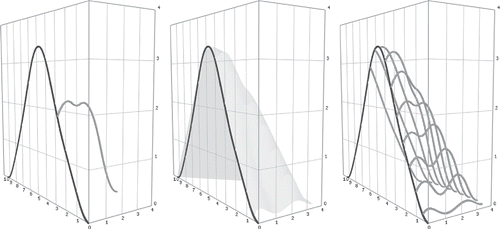
Optimal control problems operate on dynamic systems. For bilevel optimal control problems, the dynamic concept can also be added to the way in which both levels are coupled. Instead of constraining the upper level problem only at one single time point ϑ by evaluating Ψ(ξ) for ξ = x(ϑ) as in (24), it seems more straightforward to constrain it for all time points . This continuous time dependent coupling leads to an infinite number of lower level problems. Similar to the discretization method, which replaced an infinite dimensional optimal control problem by a finite optimization problem in Section 3.2, the infinite number of lower level problems of the bilevel problem is reduced to a finite number, which correspond to selected time points , , and states .

with fixedand Ψ(ξ _j ) set of solutions of

Here, v _·,j denotes the control vector v_i,j , of the lower level problem at time ξ _j and y _·,j denotes the corresponding state vector y_{i ,j} , .

If k is sufficiently large, and if the times ϑ _j , , are chosen properly, a solution of the bilevel problem with a continuous time dependent coupling can be reconstructed as follows:

Selection of adjacent solution. The change to the alternative problem, which is treated in the lower level, is caused by an unexpected event at time . Instead of considering this event immediately, the change is delayed to a time .

Application of sensitivity analysis. The numerical solution of the lower level problem for can be interpreted as the nominal solution for p 0 = ξ j of a discretized version of the perturbed optimal control problem (7). The sensitivity derivatives and can be gained using (9) and (10). Due to the continuity of the state function x(t), the parameter value is close to the nominal value p 0 for and allows approximations of type (11). Further, this continuous dependency of the solution of the lower level problem from the parameter vector of the upper level problem confirms that it is numerically reasonable to consider only lower level problems at discrete times .

After the k lower level problems are replaced by their first-order necessary conditions, one large optimal control problem remains. Due to the special type of coupling, the subsystems of differential equations x and , , can be integrated efficiently since they are independent from each other.

6. Main and alternative trajectories

The system dynamics of the crane system is given by (2). The jerks and are used as control functions, so that the corresponding accelerations can be used as boundary values. The complete system of differential equations is rewritten for the state function x(t) and the control function u(t):

(25)

The bilevel path-planning problem can be outlined as ‘move from (S ₀, L ₀) to (S_f , L_f ) and consider a possible stop for ’. For the corresponding bilevel optimal control problem, the main trajectory is calculated with respect to time and energy optimality and the alternative trajectories should stop within a fixed time minimizing the energy consumption:

(26)

with Ψ(u) set of solutions of

Each lower level problem for an alternative trajectory can be replaced by a boundary value problem using the necessary conditions. As explained in Section 4.2, for energy optimality the system of differential equations

is augmented by the system of adjoint differential equations

(27)

and the boundary conditions

For the crane system, Equation (14)(14) can be solved for the control functions of the optimal solution of the unconstrained problem:

The control functions and of the problem under box constraints , i = 1, 2 are found as in (17):

After both levels are transformed to the same time interval [0; 1], (26) reduces to:

(28)

6.1 Control-constrained lower level problem

Trajectories for the crane system were calculated for a movement from to in [m]. The numerical solution of the bilevel path-planning problem (26) is shown in Figure 3 for an equidistant discretization of r = 41 points. At the discretization points r_j  = 5 · j of the main trajectory, alternative trajectories with , , are considered with 11 discretization points.

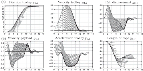
Figure 3. Optimal controls, state vectors and adjoints for main trajectory (thick line) and five alternative trajectories (thin lines) for constrained lower level control. (a) Controls, (b) States, in comparison to single-level solution (dotted line), (c) Adjoints.

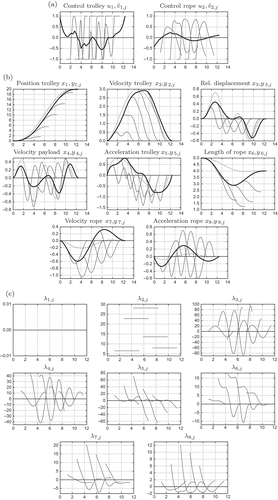
The state constraints in the upper level stay inactive. The controls for both levels are constrained by in , i = 1, 2. The controls of the lower level problems, drawn with thin lines in Figure 3(a), consist of free parts and of boundary parts, where the constraints get active. The corresponding adjoints λ_5,j and λ_8,j in Figure 3(c) exceed the interval clearly.

For reference, the solution of a path planning without considering the safety stop is drawn as a dotted line in Figure 3(b). The constraining influence of the lower level problems can be seen clearly in the curves in thick lines. The oscillating behaviour in the relative displacement of the payload is reduced slightly at the cost of taking a longer process time. The length of the rope is shortened during the main trajectory. This allows to shorten it even more in the alternative trajectories, which heightens the frequency of the swinging system and leads to more equilibrium points for the rest position.

The controls v _·,j of each lower level problem define the stop trajectories, to which a change at time τ_0,j is possible. These stop trajectories can also be calculated by solving the lower level problem starting from the system state at as a separate optimal control problem, in order to verify the bilevel method.

6.2 State-constrained lower level problem

A proper consideration of state constraints for the safety stop trajectories leads to discontinuities in the adjoints λ_·,j , whenever the constraints get active or inactive. When formulating the boundary value problems, the structures of these switching schemes have to be known.

The resulting possible function classes of y _·,j depend on the order of the state constraint. Some examples are given here, based on the differential equation systems (25) and (27).

	Constraining acceleration of trolley . The state constraint of first order allows jumps in the adjoint λ5,j , i.e. . As v 1,j is calculated from λ5,j , it is from the same function class. The jerk y 5,j is integrated from v 1,j , and therefore .
	Constraining velocity of payload . Due to the state constraint of second order, jumps in the adjoint λ4,j can appear, i.e. . It follows from the adjoint system that and therefore . Finally and are integrated from the control v 1,j .

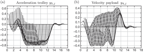
To the contrary, the results of an approximative solution for bilevel optimal control problems with state constraints in the lower level are presented in Figure 4. The constraints will be applied to the reduced optimal control problem (28), and therefore, only smooth solutions for and are found. This additional smoothness requirement in the lower level problem strengthens the constraint for the upper level problem.

Figure 4. Optimal state vectors for main trajectory (thick line) and 10 alternative trajectories (thin lines) for different state constraints in the lower level problem. (a) Constraining acceleration of trolley ; (b) Constraining velocity of payload .

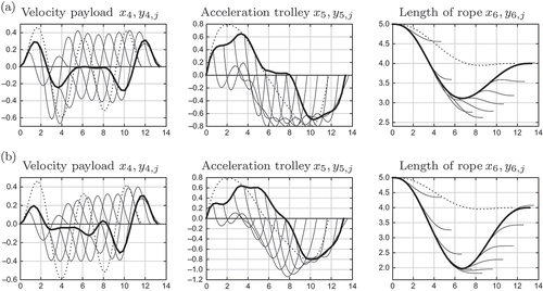
If a lower level problem is solved separately, starting from the initial value , , of the optimal solution of the bilevel problem, this leads to the same smooth trajectory – even if the state constraint is omitted. Figure 5 shows these trajectories with thick lines. Stop trajectories starting from initial values x(t) with , which were not considered during the bilevel optimization, are shown with thin lines. As they nearly hold the constraints, they can also be used for stop maneuvres at arbitrary times t.

Figure 5. A posteriori calculation of 10 old (thick lines) and 20 new (thin lines) alternative trajectories for different main trajectories. (a) Implicitly constraining acceleration of trolley; (b) Implicitly constraining velocity of payload.

6.3 Industrial solution

Asking for the existence of alternative trajectories under control or state constraints influences the oscillatory behaviour of the main trajectory and reduces the cost function

On the other hand, if the upper level problem is solved separately using as an additional (weighted) objective function, alternative trajectories with the desired constraints can be found subsequently. Figure 6 shows useful alternative trajectories, which were calculated, after the main trajectory was optimized with reduction of the oscillatory behaviour.

Figure 6. Existence of alternative trajectories for a damped main trajectory.

7. Conclusions

The path-planning problem for the movement of a crane system with alternative safety stop trajectories was presented as a bilevel optimal control problem with continuous time dependent coupling leading to an infinite number of followers. The reduction to a finite selection of followers was motivated, and by the application of necessary conditions, a conventional optimal control problem was obtained, which was solved by direct methods.

In the lower level, control constraints were considered optimally and state constraints suboptimally.

For the industrial usage, the costly solution of bilevel optimal control problems can be circumvented by formulating an adequate objective functional for the main trajectory, which allows an a posteriori calculation of the alternative trajectories.

References

- von Stackelberg , H. 1934 . Marktform und Gleichgewicht , Berlin : Springer Verlag .
- Bracken , J. and McGill , J.T. 1973 . Mathematical programs with optimization problems in the constraints . Oper. Res. , 21 : 37 – 44 .
- Dempe , S. 2002 . Foundations of Bilevel Programming , Dordrecht : Kluwer Academic Publishers .
- Bard , J. 1998 . Practical Bilevel Optimization: Algorithms and Applications , Dordrecht : Kluwer Academic Publishers .
- Chen , C. and Cruz , J.B. 1972 . Stackelberg solution for two-person games with biased information patterns . IEEE Trans. Automat. Control , 17 : 791 – 798 .
- Ye , J.J. 1997 . Optimal strategies for bilevel dynamic problems . SIAM J. Control Optim. , 35 : 512 – 531 .
- Knauer , M. 2009 . Bilevel-Optimalsteuerung mittels hybrider Lösungsmethoden am Beispiel eines deckengeführten Regalbediengeräts in einem Hochregallager , Ph.D. thesis, Universität Bremen .
- Mayrhofer , M. and Sachs , G. Notflugbahnen eines zweistufigen Hyperschall-Flugsystems ausgehend vom Trennmanöver , 109 – 118 . Seminar des Sonderforschungsbereichs 255: Transatmosphärische Flugsysteme, Technische Universität München, München, 12 December 1996, Hieronymus, München, 1997 .
- Bryson , A.E. and Ho , Y.C. 1975 . Applied Optimal Control , Washington , DC : Hemisphere Publishing Corporation .
- Ioffe , A.D. and Tihomirov , V.M. 1979 . Theory of Extremal Problems , Amsterdam : North-Holland Publishing Company .
- Pontrjagin , L.S. , Boltjanskij , V.G. , Gamkrelidze , R.V. and Miscenko , E.F. 1967 . Mathematische Theorie optimaler Prozesse , München : R. Oldenbourg .
- Neustadt , L. 1976 . Optimization: A Theory of Necessary Conditions , Princeton , NJ : Princeton University Press .
- Maurer , H. 1979 . On the Minimum Principle for Optimal Control Problems with State Constraints , Vol. 41 , Münster : Schriftenreihe des Rechenzentrums der Universität Münster .
- Hartl , R. , Sethi , S. and Vickson , R. 1995 . A survey of the maximum principles for optimal control problems with state constraints . SIAM Rev. , 37 : 181 – 218 .
- üskens , C. B and Maurer , H. 2000 . SQP-methods for solving optimal control problems with control and state constraints: adjoint variables, sensitivity analysis and real-time control . J. Comput. Appl. Math. , 120 : 85 – 108 .
- üskens , C. B . 1998 . Optimierungsmethoden und Sensitivitätsanalyse für optimale Steuerprozesse mit Steuer- und Zustandsbeschränkungen , Münster : Universität Münster, Institut für Numerische Mathematik .
- üskens , C. B and Maurer , H. 2001 . “ Sensitivity analysis and real-time control of parametric optimal control problems using nonlinear programming methods ” . In Online Optimization of Large Scale Systems: State of the Art , Edited by: Grötschel , M. , Krumke , S.O. and Rambau , J. 57 – 68 . Berlin : Springer .
- Maurer , H. and Pesch , H.J. 1994 . Solution differentiability for parametric nonlinear control problems . SIAM J. Control Optim. , 32 : 1542 – 1554 .
- Maurer , H. and Pesch , H.J. 1994 . Solution differentiability for parametric nonlinear control problems with control-state constraints . Control Cybernet , 23 : 201 – 227 .
- Malanowski , K. and Maurer , H. 1996 . Sensitivity analysis for parametric control problems with control-state constraints . Comput. Optim. Appl. , 5 : 253 – 283 .
- Malanowski , K. and Maurer , H. 1998 . Sensitivity analysis for state constrained optimal control problems . Discrete Contin. Dyn. Syst. , 4 : 241 – 272 .
- Fiacco , A.V. 1983 . “ Introduction to Sensitivity and Stability Analysis in Nonlinear Programming ” . In Mathematics in Science and Engineering , Vol. 165 , New York : Academic Press .
- üskens , C. B and Maurer , H. 2001 . “ Sensitivity analysis and real-time optimization of parametric nonlinear programming problems ” . In Online Optimization of Large Scale Systems: State of the Art , Edited by: Grötschel , M. , Krumke , S.O. and Rambau , J. 3 – 16 . Berlin : Springer .