Modelling of lateral dynamics for an endless metal process belt

Abstract

The subject of this article is the derivation of a model for lateral dynamics of an endless metal process belt. The minimal configuration of a process belt is a conveyor belt around two cylindrical return drums. In order to ensure a plane surface, the metal belt is pre-stressed to a high level. The main problem of this configuration is to guarantee perfect lateral tracking of the belt utilizing swivelling and tilting drum axes, which should guarantee a constant lateral position of the belt under all process disturbances and geometric imperfections. A dynamic process model in linear state space form is derived from simple geometric parameters of the belt and drums. Measured data from a test rig are utilized to estimate a parametric grey-box model, and both analytical and experimental models are validated against experimental results. The region of validity of the linear models is evaluated and the excellent performance of the grey-box model is demonstrated. The application of this model for control design is demonstrated for compensation of a lateral process force.

Keywords:

• steel process belt
• lateral dynamics
• grey-box model
• state space model

1. Introduction

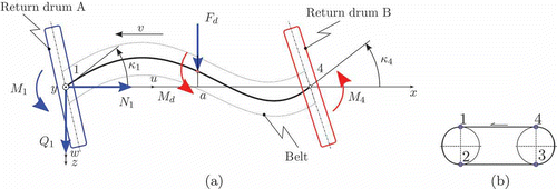
Endless metal belts are important production means for advanced processing lines and belt machines with high-quality demands. Due to the high elastic modulus E, steel process belts can only be run over cylindrical return drums especially if they are already pre-stressed to a high level [1]. Since cylindrical drums do not provide self-centring of the belt, active control with suitable actuation is necessary to ensure constant lateral positions ζ₁ and ζ₄ at the return drums (see Figure 1(a)), even in the presence of lateral disturbances.

Figure 1. Sketch of a two-drum conveyor line: (a) basic dimensions, running direction, lateral positions ζ₁ and ζ₄, and disturbances M _d and F _d ; (b) manipulated variables: swivel angles β₁ and β₄, tilting angle α.

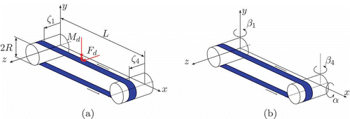
In a simple configuration the endless metal belt is running over two cylindrical return drums at each end of the conveyor line. The main problem of this configuration is to guarantee perfect tracking of the belt utilizing swivelling or tilting drum axes (see Figure 1(b)), which should guarantee a constant lateral position of the belt's edges under all process disturbances and geometric imperfections.

In literature only few publications are dedicated to this problem: a number of patents (e.g. [2,3]) present means for controlling the lateral belt position. However, no mathematical model for the lateral belt dynamics is given. Since the late 1990s mathematical models for this problem have been designed, which are based on the assumption that the lateral deformation of the belt can be modelled by a beam [4]. In similar application-oriented questions that deal with elastic slim long structures, the Euler–Bernoulli model could be used successfully. As opposed to these models [5,6], the dynamic part of the beam could be neglected because of the low longitudinal belt speed. But due to the high longitudinal pre-stress, second-order bending theory was employed. The complex friction conditions between belt and drums resulted in the development of non-linear models [7]. Recently, a finite element model has been developed [8], which is accurate but not suitable for control design and analytical representation of the lateral belt dynamics. Test rigs of different sizes have also been developed to validate the models experimentally [9]. Those models can be considered mature by now since they can reproduce measured data at a high accuracy. However, they were merely designed for the purpose of predicting the lateral position of the belt offline in the time domain [1,10]. To this end, geometric parameters of the process as well as material parameters of the belt have to be known, a non-linear friction model for the contact between belt and drums is necessary, and the transport delay for the duration of contact between belt and drum is mostly neglected. Moreover, an iterative solution of the complex model equations is necessary at each single time step.

The model presented in this article represents an extension to the models from [7,10,11] and a detailed derivation can be found in [12]. The extension is threefold:

1.	The number of model parameters is reduced to two readily available geometric values (diameter of drum and length of conveyor line) plus an adjustable transport delay.
2.	Due to the linear state space structure the proposed model is perfectly suited for controller design, and it can also be implemented online in model-based control schemes.
3.	The transport delay of the belt on the drums is explicitly considered and can be used for tuning the model dynamics.

Although only linear relations are utilized and a purely kinematic transport on the drums is assumed, the validation using experimental data from a test rig shows an excellent fit to measured data.

The remainder of the article is structured as follows: Section 2 presents the analytical model structure of the lateral belt dynamics. Special attention is paid to the kinematic transport on the drums and the resulting state space model is given in an analytical representation. Section 3 states the methods for retrieving experimental data. Section 4 demonstrates, that both open-loop and closed-loop experiments show excellent agreement between simulation and measurements. Section 5 provides the conclusions and an outlook on future work.

2. Modelling of lateral belt dynamics

The modelling approach presented in this article is partitioned into the following sections: First, some assumptions followed by fundamental principles are given. Then, the static flexible deformation w(x) of the belt between the drums is derived from the geometric boundary conditions by using the Euler–Bernoulli equation. Finally, the kinematic transport of the belt on the drums is modelled by a transport delay. The resulting model of lateral dynamics of the belt depends on the belt's travel s _b  = R φ only and is given in state space representation.

2.1. Assumptions

The following assumptions are in agreement with practical implementations of metal belts and facilitate the analytical modelling:

1.	The main mechanism for lateral dynamics is the quasi stationary deflection of the belt in a lateral direction.
2.	All forces (single loads) act in-plane with the belt (xz-plane); all bending moments act orthogonal to the belt plane (y-direction, see Figure 1(a)).
3.	The belt is reduced to an infinitely small beam in the lateral direction, utilizing the area moment of inertia of the original belt geometry.
4.	Perfect adhesion between belt and drums exists.
5.	Buckling or other instabilities do not occur.

Assumption 1 has been experimentally verified by [7,13]. Assumption 2 is valid because due to the high pre-stress only small deflections normal to the belt plane are possible, and as shown in Sections 2.3 and 2.4 do not affect lateral dynamics. Assumptions 3–5 are justified by the high pre-stress of the belt (up to 0.8 R _e , where R _e denotes the material's yield strength).

2.2. Model variables

The system variables can be grouped into manipulated variables, output variables and disturbances (see Figure 1):

•	Manipulated variables: Swivel angles β1 and β4 of the drums, and drum axle crossing by tilt angle α of one drum.
•	Output variables: Lateral displacements ζ1 and ζ4 of the belt at the drums.
•	Disturbances: Single force F d , acting in z-direction at coordinate x = a, and single bending moment M d , acting in y-direction at coordinate x = a.
•	Independent variables: Time t in time domain and rotation angle of drum φ or belt travel s b  = R φ in spatial domain.

Remark 1:

The co-location of disturbances at coordinate x = a is introduced for the sake of brevity; as can be seen from the results in Sections 2.4 and 2.7, the extension to multiple disturbances at different coordinates is straightforward.

2.3. Fundamental principle of lateral motion

Assuming perfect adhesion between belt and drums (Assumption 4), the longitudinal belt speed v(t) at a drum with radius R is given by Equation (1)(1) (compare to Figure 2):

(1)

Figure 2. Situation of lateral belt position ζ for a swivel angle β and a thread slope θ in the horizontal x–z plane. For the belt angle with respect to absolute coordinates κ = θ + β holds. The tangent to the belt's centre line at the point of first contact is denoted by T.

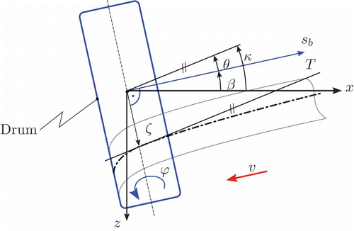
Based on this assumption, the lateral movement of the belt at the point of first contact between belt and drum can be derived by Equation (2)(2):

(2)

Linearization of Equation (2)(2) for small angles θ _i at the operating point θ _i  = 0 leads to the simple relations

(3)

where w(x) denotes the lateral elastic deformation of the belt (see Figure 3). Equations (3)(3) state that the belt is moving in a lateral direction like a conveyor screw with a thread slope of θ _i  = κ _i – β _i for stationary boundary conditions.

Figure 3. Sketch of a two-drum conveyor line: (a) variables of the deformed belt: sketch of the conveyor belt modelled by an elastic beam; (b) indices of the belt system related to running direction.

2.4. Elastic deformation of the pre-stressed belt

The goal is to find an equation describing the elastic deformation w(x) of the belt subject to the geometric boundary conditions w(0), w(L), w′(0) and w′(L), where w(0) and w(L) are the lateral deflections of the belt at the bending (point 1) and driving drums (point 4), respectively (see Figure 3). The swivel angles of the drums are denoted by β₁ and β₄, and the belt's angles in absolute coordinates are given by κ₁ and κ₄.

Neglecting the dynamics of the beam (Assumption 1), the flexible static deformation between the points 1 and 4 is given by an ordinary differential equation (ODE, Euler–Bernoulli) [14,15]

(4)

where G is the shear modulus, J _y is the area moment of inertia and η is a dimensionless form factor [15]. Calculation of the bending moment M at the subsections I and II in accordance with Figure 4 leads to Equations (5)(5) and (6)(6)

(5)

(6)

where N ₁ and Q ₁ denote the longitudinal and shear forces at point 1, respectively. For both sections holds. Note that the disturbances F _d and M _d are explicitly contained in Equation (6)(6). The deflection caused by the swiveling drums is obtained by inserting the inner bending moments into Equation (4)(4) and considering that w _I (a) = w _II (a) and w′ _I (a) = w′ _II (a) must hold:

(7)

Figure 4. Sketch of the upper belt plane: the belt is split into subsections (a) I and (b) II. M ₁, N ₁, Q ₁: moment, longitudinal and shear forces at point 1. M _I , M _II : inner bending moments in sections I and II.

Since N ₁ < 0 (tensile force), the following definition for the coefficient ν of w in Equation (7)(7) holds:

(8)

Utilizing Equation (8)(8), Equation (7)(7) can be rewritten as

(9)

A piecewise solution of the ordinary linear inhomogeneous differential equation (ODE) of Second-order Equation (9)(9) is given by

(10)

The geometric boundary conditions at the drum contact points are given by

(11)

and the continuity conditions between the two sections are given by

(12)

Linearizing the boundary conditions Equation (11)(11) at the operating point β _i  = 0, κ _i  = 0, and utilizing Equation (3)(3) the ODE Equation (7)(7) can be expressed by the geometric boundary conditions and disturbances only:

(13)

The coefficients K _i are given in Appendix, Equation (A2)(A2); note that K _i  = K _i (N ₁, L, a) holds for all i = 1, …, 6. The ODE for the lower belt is obtained by an exchange of indices (1 → 3, 4 → 2) and setting F _d  = 0 and M _d  = 0:

(14)

Remark 2:

If the pre-stress is neglected (N ₁ = 0), the ODE Equation (7)(7) can be simplified accordingly and the piecewise solutions Equation (10)(10) are polynomials in x. In this case the formal structure of Equations (13)(13) and (14)(14) remains unchanged, however, the individual coefficients K _i will no longer depend on N ₁ (K _i  = K _i (L, a), see Appendix, Equation (A3)(A3)).

2.5. Transport delay

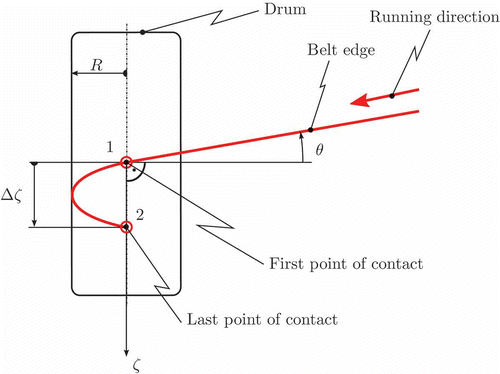
A speed-dependent time delay is a typical characteristic of belt systems. By modelling in the spatial domain, this problem is transformed into a speed-invariant transport delay, which is caused by the belt's transport over half the drum's circumference (see Figure 5). For the stationary conditions shown there, Δζ = Rπ tanθ holds. This result shows that the transport on the drums considerably adds to the lateral belt dynamics. Figure 5 clearly shows a transportation lag from point 1 to 2. The delay s _b,12 in the spatial domain is given for hemicycle loop by s _b,12 = Rπ = s _b,34. A representation of the transport delay in Laplace domain can be found in Equation (15)(15) (s denotes the Laplace variable). In order to derive a linear minimum phase-shift model, this transport delay is approximated by a Padé-approximation [16]:

(15)

Figure 5. Transport delay and coupling between upper and lower belt as a consequence of hemicycle transportation on drum. Thread slope θ, drum radius R and lateral displacement Δζ are shown.

The corresponding equation of a first-order Padé-approximation in the spatial domain is given by

(16)

By a simple exchange of indices (1 → 3, 2 → 4) Equation (16)(16) also describes the delay at the second drum.

2.6. Effect of tilt angle α

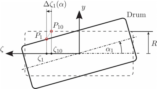
For a given tilt angle α a lateral displacement Δζ(α) will result according to Figure 6, which can be linearized for α ≪ 1:

(17)

Figure 6. Geometric relations at tilted drum: tilt angle α₁ causes a lateral displacement of Δζ₁(α). Dashed line: drum position at operating point. Solid line: tilted drum. P ₁₀: contact point in original position. P ₁: contact point in tilted position. ζ₁₀: original lateral displacement. ζ₁: tilted lateral displacement.

Superposition of swivel and tilt angles extends Equations (13)(13) and (14)(14) to

(18)

2.7. State space model

Based on Equations (16)(16) and (18)(18) the complete lateral belt dynamics can be described, where the only independent variable is the belt's travel s _b . A suitable state vector x is defined by

(19)

The corresponding linear state space representation of sixth-order in the form

(20)

is given by

(21)

In Equation (21)(21) the manipulated variables u of an active control are the angles of the drums β₁, β₄ and α₁, and the disturbance inputs d are given by the lateral force F _d and a bending moment M _d . The model output y is given by ζ₁ and ζ₄, which denote the lateral belt positions at the drums. The matrices D and F of the output equation (20)(20) are zero matrices of appropriate dimensions.

2.8. Static influence of manipulated variables

As can been seen in the entries of the B matrix in Equation (21)(21), the manipulated variables swivel β versus tilt α angles act on the same system state derivatives, but have different static gains K _β and K _α. The relative static influence is therefore given by and . Inserting from Equation (A3)(A3) and using the numerical values from the testrig Section 3.1, it follows that the swivel angle is 1.96 times more effective than the tilt angel for the given set-up.

3. Measurement and identification

3.1. Test rig and measurement setup

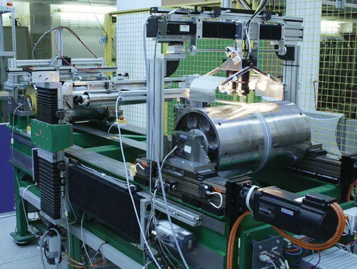
The experimental set-up consists of two drums with radius R = 0.17 m, a centre distance of L = 2 m and an endless metal belt with a width of b = 0.125 m (Figure 7). The supporting points for the bearings of the return drum can be adjusted independently by two linear drive units. A dedicated PID-controller guarantees a constant mean longitudinal stress in the belt by synchronous adjustment of the linear units. Input to this control loop are the measured longitudinal reaction forces in the bearings [17]. An anti-parallel adjustment of the units generates a swivel angle β of the drum (see Figure 2). The lateral position of the belt is measured at both drums with independent measurement systems [18]. The whole test rig is fully automated and operated via a realtime measurement and control system. All data are recorded with a fixed sampling time of T _s = 0.018 s. A more detailed description of the test rig can be found in [9].

Figure 7. Automated test rig for lateral dynamics of an endless metal belt.

Since data are originally sampled in the time domain, a conversion to spatial domain is necessary:

(22)

In order to obtain an equidistant spatial sampling distance s _b,s , speed-dependent re-sampling has to be performed with a suitable constant factor k _s :

(23)

To remove outliers and to compensate for the periodic disturbance of the imperfect belt edges additional post-processing of measured data is necessary. A detailed description of this process can be found in [12,16].

3.2. Identification procedure

For the purpose of validation and comparison, both non-parametric and parametric models have been identified from measured data using the Matlab identification toolbox [19]. A correlation analysis was performed in order to estimate the impulse response of the system. This non-parametric model in the time domain was also utilized for validating the system's adjusted transport delay s _adj (Section 4.2). Additionally, a non-parametric estimate of the system's frequency response was performed using Welch's method [20].

4. Validation

4.1. Time domain validation: step responses

After adjusting the swivel angle β₁ for stationary operation, a step input Δβ was added, causing the belt to change its lateral position with constant lateral velocity after transient dynamics have decayed (integral action, see Figure 8). Step responses were recorded in both directions for increasing step sizes. Table 1 lists the slope of the step responses and the static gain of the respective transfer function for both directions with respect to the input step size |Δβ|. The measured gain values show that symmetry of the control action is ensured. A 95% confidence interval for the estimate of the mean static gain of the transfer function is therefore given by 2.48 ± 0.178, which amounts to a relative uncertainty of 7.2%. It is consequently safe to assume that a universal static gain of 2.48 is valid for all input step sizes. This is also a strong evidence for the assumption of linear behaviour.

Figure 8. Measured step responses for different swivel angle step inputs Δβ in °. Results for both positive and negative input amplitudes are shown. Sampling in spatial domain s _b,s  = 0.1 m.

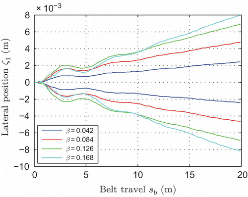
Table 1. Stationary values for step responses with increasing step size

Step size |Δβ|	Positive slope	Negative slope	Positive gain	Negative gain
0.042°	0.106	−0.098	2.49	2.29
0.084°	0.212	−0.205	2.53	2.42
0.126°	0.320	−0.314	2.55	2.47
0.168°	0.433	−0.428	2.57	2.53
Note: Slope values are listed in and gain values are given in .

4.2. Empirical parameter adjustment

The stationary solution of the analytical model Equation (20)(20) for β₄ = α = 0, F _d  = 0 and M _d  = 0 is given by [16]

(24)

The assumption of s _b,12 = s _b,34 and rearranging Equation (24)(24) yields an explicit formula for an empirical transport delay:

(25)

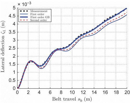
Inserting the data from Table 1 into Equation (25)(25) yields the values given in Table 2. Although a small systematic deviation between and is visible, a value of s _b,adj = 479 mm yields excellent results when compared with measured data (see Figure 9). The purely analytical model with N ₁ = 0 and transport delay s _b,12 = 530 mm Equation (A3)(A3) exhibits a small stationary off-set but also features high accuracy for the oscillating behaviour of the belt and static gain. The more complex model with N ₁ ≠ 0 is more accurate, however, it does not achieve the performance of the grey-box model.

Table 2. Identification results of s _b,adj for different step sizes

Step size |Δβ|	(mm)	(mm)
0.042°	467	680
0.084°	430	536
0.126°	409	485
0.168°	397	426

Figure 9. Validation in spatial domain: step response to swivel angle Δβ₁ = 0.042: measurement: measured signal of ζ₁, first order: beam with N ₁ = 0, second order: beam with N ₁ ≠ 0, first order GB: grey-box model utilizing s _adj.

Remark 1:

The fact that s _b,adj < s _b,12 suggests that Assumption 4 (perfect adhesion between belt and drum) is only partially valid. This means that the lateral displacement Δζ in Figure 5 will be smaller due to slip between belt and drum.

4.3. Frequency domain validation: Bode plot

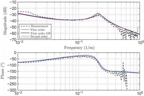
The dynamic behaviour of the analytical model is in close agreement with measured data as confirmed by the frequency response. Bode plots from the analytic model, the grey-box model and a non-parametric estimation are shown in Figure 10. An excellent agreement between these models can be seen, and only the frequency and damping of the resonance peak is slightly offset in the simple analytical model as well as a small offset in the low-frequency range exists.

Figure 10. Validation in frequency domain: measurement: measured signal and spectral estimation of ζ₁, first order: beam with N ₁ = 0, second order: beam with N ₁ ≠ 0, first order GB: grey-box model utilizing s _adj.

4.4. Padé-approximation

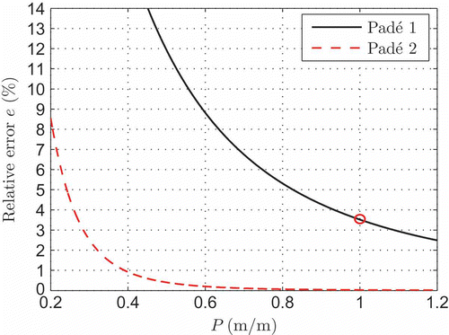
By defining a relative phase error e the quality of the proposed Padé-approximation (see Section 2.5) can be validated. It is defined by e = (φ_Padé − φ₁₂)/φ₁₂, and for a given drum radius R a relationship between this relative phase error e and the period length of the belt dynamics (where f is the spatial eigenfrequency of the belt's lateral motion) can be represented graphically.

From Figure 11 it is quite obvious that the Padé-approximation of first order (black line) only yields a phase error of 3.5% at the most relevant cycle duration (compare Figure 9) of P = 1. A Padé-approximation of second order (dashed red line) achieves an even smaller error, however, this accuracy is not effective due to the increase in model order.

Figure 11. Relative phase error e of the Padé-approximation with respect to normalized period P of lateral belt dynamics.

4.5. Invariance to force N ₁

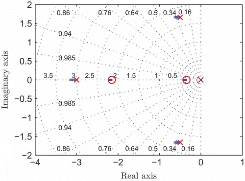
The variation of poles and zeros is more closely investigated by a root locus plot parameterized by the force N ₁ in Figure 12. In this plot N ₁ is varied such that the longitudinal stress in the belt varies between zero and R _e (R _e being the material's yield strength). The dominant (close to the imaginary axis) poles and zeros of both models remain almost identical, and the remaining poles and zeros show minimal deviations.

Figure 12. Pole zero plot of analytical model parameterized by force N ₁. A cross denotes a pole (large red crosses designate the poles for N ₁ = 0) and a circle marks a zero (large red circles designate zeros for N ₁ = 0).

4.6. Closed-loop disturbance response

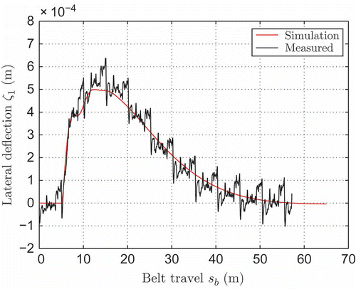
In Figure 13, the closed-loop step response of the controlled belt machine to a step input of a lateral disturbance force F _d is plotted (F _d  = 30 N at t = 5 s). Again, the simulation of the grey-box model yields an almost perfect prediction of the real system behaviour. Note that the measured lateral position ζ₁ exhibits a distinct periodic deviation (meander), which is due to production imperfections of the used belt.

Figure 13. Lateral step disturbance F _d at t = 5 s and closed-loop response.

5. Conclusion

A new grey-box model for the lateral dynamics of an endless steel process belt has been presented. Control inputs are the horizontal swivel angles and vertical tilt angles of the return drum, disturbance input is a lateral force and a disturbance moment to one strand, and outputs are the lateral strip positions at the drums. The model is simple yet very accurate: it is linear, in state space form, computationally inexpensive, but due to an adjustable transport delay parameter it can be tuned to excellent accuracy. All of the few other parameters are easily available and allow for an efficient and straightforward modelling procedure. In contrast to existing model structures [7,8] the proposed model does not need any physical parameters on friction, and no iterative solvers are necessary. The excellent accuracy of the model is demonstrated by a comparison with measured results from an experimental belt machine. These data are also utilized for identification of a non-parametric model and for a comparative validation of all models. These results clearly show that the assumption of linear system behaviour is justified and that the longitudinal force N ₁ may be neglected. It is further shown that both analytical and black-box models are consistent and capture the linearized dynamics of the process. Therefore, the presented analytical model can serve for the dynamical prediction of belt machines still in the design phase as well as a basis for design of a lateral position controller.

Future work will be dedicated to a more general disturbance model, an investigation on the effects of varying disturbance positions, additional control inputs and modern model-based control methods. Due to the simple linear structure this model could be used directly for the dynamic layout of the actuators by the method of inverse simulation [21].

Acknowledgements

This work was financially supported by FFG, project number 813006/12016. The authors thank the Institute of Engineering Design and Technical Logistics, Vienna University of Technology, for furnishing the test rig and measurement support.

Appendix

Utilizing ν from Equation (8)(8) and defining μ by

(A1)

the coefficients in Equation (13)(13) can be calculated as given by Equation (A2)(A2):

(A2)

As mentioned in Remark 2 the resulting expressions for N ₁ = 0 are simplified to

(A3)

References

- Egger , M. 2000 . SeitlichesLaufverhaltendesFördergurtesbeimGurtbandförderer , Ph.D. thesis, Vienna University of Technology . In German
- K. Yasunori, JP62104617 (A): Meandering correcting device for strip, May 1987. ECLA: B21B41/00 IPC: B21B39/14; B21B41/00; B21B41/06; (+4).
- Y. Junichi and Y. Shunichi, JP2008063019 (A): Endless steel belt meander correction device, and film formation device, March 2008. ECLA: IPC: B65H23/038; B05C5/00; B65H23/032; (+1).
- Egger , M. and Hoffmann , K. 2004 . Flat belt conveyor . Proceedings of the First Cappadocia International Mechanical Engineering, CMES, Cappadocia, Urgup, Turkey . July 14–16 2004 . pp. 6 Nigde , , Turkey : Department of Mechanical Engineering, Nigde University .
- Bachmayer , M. , Ulbrich , H. and Rudolph , J. 2011 . Flatness-based control of a horizontally moving erected beam with a point mass . Math. Comput. Model. Dyn. Syst , 17 ( 1 ) : 49 – 69 .
- Zrnic , N.D. , Bosnjak , S.M. and Hoffmann , K. 2010 . Parameter sensitivit analysis of non-dimensional models of quayside container cranes . Math. Comput. Model. Dyn. Syst , 16 ( 2 ) : 145 – 160 .
- Egger , M. , Pirko , A. and Hoffmann , K. 2007 . Simulation of flat belt running . Steel Res. Int , 78 ( 4 ) : 364 – 368 .
- Koller , M. 2009 . Simulation des seitlichen Verlaufens von endlosen Stahlbändern , Master's thesis, Vienna University of Technology . In German
- Hoffmann , K. , Pirko , A. and Grosz , H.C. Enhancement of belt conveyor test stand . Abstracts of 21st Danubia-Adria Symposium on Experimental Methods in Solid Mechanics . 29 September–2 October , Brijuni/Pula , Croatia.
- Ritzinger , P. 1997 . Seitliches Bandlaufverhalten von langsam laufenden Metallbändern auf zylindrischen Trommeln , Ph.D. thesis, Vienna University of Technology . In German
- Pirko , A. 2006 . Untersuchungen zur Gurtf¨uhrung mit geregelten Schrägrollen , Ph.D. thesis, Vienna University of Technology . In German
- Schulmeister , K.G. 2009 . Modellierung und Regelung des lateralen Laufverhaltens von Stahl-prozessbändern , Ph.D. thesis, Vienna University of Technology . In German
- Schulmeister , K.G. and Kozek , M. Modeling of lateral dynamics for an endless steel belt . Proceedings of ISCM II and EPMESC 2009, International Chinese Association for Computational Mechanics . 30 November–3 December , Hong Kong, Macau , China.
- Kreyszig , E. 1983 . Advanced Engineering Mathematics , New York : John Wiley and Sons .
- Parkus , H. 1995 . MechanikderfestenKörper , New York : Springer-Verlag . In German
- Schulmeister , K.G. and Kozek , M. 2009 . Modelling of lateral dynamics for an endless steel process belt . Proceedings of MATHMOD09, Vienna University of Technology . February 11–13 2009 , Austria. Edited by: Troch , I. and Breitenecker , F. pp. 294 Vienna : ARGESIM Publishing House .
- Pirko , A. , Egger , M. and Hoffmann , K. 2006 . Flat steel belt guiding mechanism . Proceedings of Advanced Engineering Design (AED 2006), 5th International Conference on Advanced Engineering Design, Prag , 11–14 June
- Gabmayer , T. , Hoffmann , K. and Decker , K. Optical measuring system to acquire and control the position of running metal bands . 24th DANUBIA-ADRIA Symposium on Developments in Experimental Mechanics, Lucian Blaga – University of Sibiu . September 19–22 , Romania. pp. 67 – 68 . Vienna : Danubia Adria Society on Experimental Methods .
- Matlab system identification toolbox, 2008. http://www.mathworks.com/help/toolbox/ident/ (http://www.mathworks.com/help/toolbox/ident/) (Accessed: 25 May 2011 ).
- Ljung , L. System Identification: Theory for the User . Prentice Hall . Englewood Cliffs , NJ .
- Murray-Smith , D.J. 2011 . Feedback methods for inverse simulation of dynamic models for engineering systems applications . Math. Comput. Model. Dyn. Syst , 17 ( 5 ) : 515 – 541 .
Appendix
Utilizing ν from EquationEquation (8)(8) and defining μ by