The application of parameter sensitivity analysis methods to inverse simulation models

Abstract

Knowledge of the sensitivity of inverse solutions to variation of parameters of a model can be very useful in making engineering design decisions. This article describes how parameter sensitivity analysis can be carried out for inverse simulations generated through approximate transfer function inversion methods and also through the use of feedback principles. Emphasis is placed on the use of sensitivity models and the article includes examples and a case study involving a model of an underwater vehicle. It is shown that the use of sensitivity models can provide physical understanding of inverse simulation solutions that is not directly available using parameter sensitivity analysis methods that involve parameter perturbations and response differencing.

Keywords:

• parameter sensitivity
• inverse simulation
• sensitivity model
• underwater vehicle

1. Introduction

An inverse dynamic model generates a set of time histories of inputs to provide specified time histories of selected output variables of the model. In terms of practical applications, this method could involve finding the inputs needed to allow a fixed-wing aircraft, helicopter or marine vehicle to perform a specified maneuver or the inputs needed to allow a robotic arm to follow a given trajectory [1].

In an engineering design context, inverse solutions have been found to be particularly relevant in applications where actuator performance is important and where design decisions have to be made about the size and shape of control surfaces or of engines, motors and other elements within drive-train systems. This is a situation that arises very commonly in aircraft, marine and land vehicle designs (see, e.g. [1–3]). If, for example, results from an inverse model of a vehicle or robot show that inputs cannot be found that allow a specified maneuver to be performed, changes must be made in terms of either the required maneuver or the design of the hardware and software of the system itself. Knowledge of the sensitivity of inverse solutions to variation of parameters of a model can be of considerable value in making these design decisions.

In the case of single-input single-output (SISO) linear minimum-phase models, a process of transfer function inversion can lead directly to an inverse description. In cases where the order of the numerator of the original transfer function is the same as the order of the denominator, this inverse model can be implemented directly as an inverse simulation. In most situations that arise in practice this is not the case, and in order to make the inverse model realizable, one or more additional poles must be introduced. These additional ‘propering’ poles must be positioned in the s-plane at points (in the left-half plane) that are far from the positions of poles and zeros of the model. This approach is described by Buchholz and von Grünhagen who have applied this type of methodology not only to SISO models but also to multi-input multi-output (MIMO) linear models [4].

Analytical methods of model inversion can be applied to some forms of linear model and techniques of model inversion have been developed for the non-linear case [5,6]. Such models require transformation to linear and controllable descriptions using non-linear state feedback together with concepts from differential geometry. Other mathematical techniques, such as regularization, are also relevant. However, although successful in some advanced applications involving automatic control [7,8], these analytical methods for non-linear systems have not been used extensively in engineering design, in part, perhaps, because they involve specialist mathematical methods and concepts that are not widely used in most areas of engineering.

Approaches based entirely on simulation have been found to offer an interesting and attractive alternative to analytical methods of model inversion. Several inverse simulation methods have been developed, which involve the use of iterative numerical methods [1,2], and such methods can be computationally intensive in the case of complex non-linear models. Although these numerical approaches have origins in specific areas of engineering application, they are applicable, in a general way, to many forms of linear and non-linear mathematical models. For example, methods of this kind developed initially for helicopter flight mechanics and pilot handling qualities investigations have been applied very successfully in other areas such as ship steering control systems analysis [9].

A completely different approach, based on feedback principles [4,10], has a long history that is linked to the use of feedback methods in generating inverse functions on analogue computers. Essentially, this involves the creation of a high-gain feedback pathway around the model for each output variable of interest. The patterns of the reference signals for each of these feedback loops then form the required time histories of the corresponding output variables. The inverse solution is obtained from the signals at the inputs to the model, provided the gain of each feedback loop is high enough over the frequency range of interest. Recent experience has demonstrated that this feedback-based approach can be applied successfully for many different linear and non-linear inverse simulation applications involving SISO and MIMO non-linear models and can show benefits in terms of computational efficiency compared with the more-established iterative methods [10]. Although high-gain proportional feedback is acceptable in many cases, the principle of feedback-based model inversion applies also to other forms of feedback structure, and the approach is not limited to proportional control methods. Analysis of a linearized version of the given model using frequency domain or root locus methods of analysis can provide useful additional insight about the properties of the feedback loops and may allow parameters of the controller block to be adjusted to ensure that poles of the linearized inverse simulation model lie at points in the s-plane close to the zeros of the forward model. Branches of the root locus that tend towards infinity in the s-plane as the gain factor becomes large can be identified and their effect on the inverse simulation can be investigated.

This article presents a number of approaches to the sensitivity analysis of inverse simulation models. Particular emphasis is placed on methods that provide physical insight and computational efficiency, in terms of both the sensitivity analysis and inverse simulation techniques involved.

2. A brief review of parameter sensitivity analysis concepts and methods

Parameter sensitivity analysis techniques are important for establishing how responses of a model change when parameters are varied. In particular, parameter sensitivity analysis can show which model parameters have most effect on the model behaviour and which parameters have little or no influence [11,12]. Models are never exact and it is important to be able to assess parametric dependencies at the model development stage as part of an investigation of modelling assumptions, simplifications and overall credibility.

Sensitivity information is also very important for system optimization in engineering design, and it should be noted that methods of optimization based on gradient methods make direct use of parameter sensitivity measures. The sensitivity may be characterized in a number of ways using time-domain or frequency-domain performance measures [12]. Information about parameter sensitivities, when taken together with structural information, can also be of considerable value in experimental modelling and, more generally, in the iterative development and refinement of complex system models using test data from real systems.

Research by Tomović and his colleagues at the University of Belgrade [11,13,14] has provided the foundation for much of the published work on sensitivity analysis of dynamic models. Important contributions have also been made by Frank [12] and others, including Rosenwasser and Yusupov [15].

Central to sensitivity analysis methods is the concept of the sensitivity function. This is defined through a Taylor series expansion. For example, in the time domain, if is the response of a chosen variable of the model and this is a function of time (t) and a parameter q, the difference between a response , where q has the particular value , and a response , where the parameter q takes a new value , is given by

(1)

If is sufficiently small it follows that

(2)

The quantity is known as a first-order sensitivity function for the chosen variable y(t). Truncation of the series after the second term introduces a form of linearization and allows the superposition principle to be used to find the effect of simultaneous changes of the values of several different parameters. For state-space models, this concept of a parameter sensitivity function may be extended to the trajectory sensitivity function , where x is the vector of state variables.

The relative sensitivity function is a useful measure for making quantitative comparisons of the influence of different parameters. If all these involve the sensitivity of one specific model variable x to a number of different parameters, an appropriate measure of relative sensitivity is given by . For cases involving several variables a dimensionless form of measure may be more useful, where the quantity x_mj is some representative value of the variable x_j , such as the peak or mean-squared value.

2.1. Estimation of sensitivity functions using repeated solutions

From Equation (2)(2), it is possible to write:

(3)

The use of this finite difference approximation requires two repeated simulation runs and the selection of an appropriate parameter perturbation Δq. The accuracy of the estimation depends on the choice of Δq, and tests may need to be repeated for several trial values of Δq to establish an appropriate value. A separate sensitivity function evaluation must be made for each parameter that is of interest.

The main weakness of this approach is associated with the fact that it requires taking the difference between two solutions. If these solutions have inherent numerical errors ϵ₁(t) and ϵ₂(t), it follows that

(4)

As Δq is small, the error due to the term ()/Δq may be significant. A more important problem with this method is that, for many types of engineering applications, it is purely a numerical process and does not provide any physical insight with regard to the sensitivity function.

2.2. Determination of sensitivity functions using sensitivity models

If a general form of non-linear dynamic model is described by a set of equations:

(5)

(6)

where are state variables, are inputs and are the variables of interest, the sensitivity of the system to variation of a parameter q may be found by partial differentiation. This process gives a set of sensitivity equations that can also be termed as the sensitivity model.

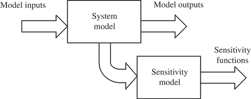
When solved in conjunction with the system model equations, these sensitivity equations provide solutions for the sensitivity functions. The sensitivity equations are, in general, linear ordinary differential equations with time-varying coefficients. Figure 1 is a schematic diagram that represents the process of generating sensitivity functions using this approach. The structure of the sensitivity model is directly related to that of the system model in the case of a linear model with constant coefficients. However, for each selected variable, a given model must have as many sensitivity models as the number of parameters of interest, although, for particular cases, methods have been developed that allow simultaneous estimation of many sensitivity functions using a single sensitivity model [16].

Figure 1. Block diagram illustrating the relationship between the system model and the corresponding sensitivity model for the general case of a multi-input multi-output system model.

Initial conditions for sensitivity models are, in most cases, zero. Non-zero initial conditions can arise, for example, in the sensitivity models for cases in which the system model has a variable structure and such issues are discussed in more detail by Frank [12].

3. Sensitivity models in inverse simulation solutions for linear models

Although parameter sensitivity analysis is of special interest in the case of models involving non-linearities, direct use of the sensitivity model approach is of limited usefulness due to the complex nature of the resulting sensitivity equations. In addition, physical insight that can be gained from the sensitivity model in the non-linear case is often rather limited. More useful information about a non-linear model can often be obtained from sensitivity analysis of linearized forms of description, although this may require the investigator to bring together results for a number of different operating conditions.

3.1. Sensitivity analysis for inverse simulation models based on transfer function manipulation

3.1.1. The SISO case

Consider a linear time-invariant system model G(s) described by a transfer function involving numerator and denominator polynomials A(s) and B(s), respectively, such that:

(7)

where U(s) represents the Laplace transform of the model input and Y(s) represents the Laplace transform of the model output. The inverse model is given by

(8)

and for this inverse model to be realizable it is essential that the order of the polynomial A(s) be equal to or greater than the order of B(s). This can be guaranteed if the original model is modified slightly through the introduction of a multiplicative term P(s), which is of sufficient order to give a denominator polynomial A(s)P(s) in the inverse model having the same order as the polynomial B(s). In the context of inverse simulation, the introduction of this polynomial P(s) makes the inverse model ‘proper’ and it should be chosen so that the additional poles in the inverse model lie far from the positions of the poles and the zero of G(s). In practical terms, this should be typically at least 100 times further from the origin of the s-plane than the other poles and zeros. If the polynomials A(s) and B(s) are of the same order the additional polynomial P(s) is unity. The introduction of this additional multiplicative factor P(s) gives an inverse model of the form:

(9)

where

(10)

The variable Y(s) in the inverse model is defined as the output required from the model and its form is chosen by the user. It is thus possible to find the sensitivity of the variable U(s) to any parameter q of the model G(s) by differentiating Equation (9)(9) partially with respect to q, taking Y(s) as independent of q.

This gives

(11)

But

(12)

and if Y(s) is a time history specified by the investigator and therefore independent of q, as stated above, the right-hand side of this equation must also be independent of q. Thus, it can be shown that

(13)

and therefore the block diagram relating the inverse simulation model and the sensitivity model is as shown in Figure 2.

Figure 2. Block diagram of inverse model and sensitivity model for the case of a linear time-invariant model described by a realizable inverse transfer function 1/G*(s).

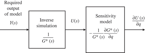
For a parameter q, which appears both in the denominator and in the numerator of G(s), it can be shown that

(14)

If we are also interested in establishing the sensitivity of the inverse model to a parameter q associated with the polynomial P(s), the approach used is identical to that applied above and it can be readily shown that

(15)

Example:

A linear SISO system is described by a transfer function given by

(16)

where the nominal parameter values are K = 10, a = 1, b = 1 and c = 1.

Sensitivity analysis using the sensitivity model approach of Equation (14)(14) gives the following expressions for the sensitivity functions for the inverse model:

(17)

(18)

(19)

(20)

Examination of these equations provides some interesting information about the sensitivity functions. For example, the sensitivity model for parameter a is of first order, whereas those for parameters b and c are of second order. In addition, the sensitivity functions for parameters b and c are related, because Equations (18)(18) and (19(19)) show that is the derivative of . Such information can provide valuable physical insight in terms of differences in effects of the parameters of the forward model on the inverse simulation.

It should be noted that the order of the numerator of the transfer function in Equation (16)(16) is 1 and the order of the denominator is 2 and, thus, the ideal inverse model is unrealizable. For the purposes of model inversion an additional component of order 1 is therefore required and it is chosen to be

(21)

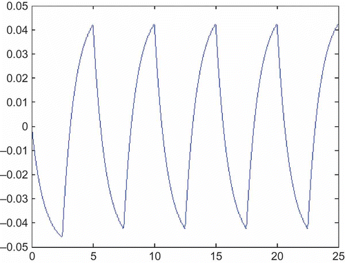
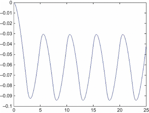
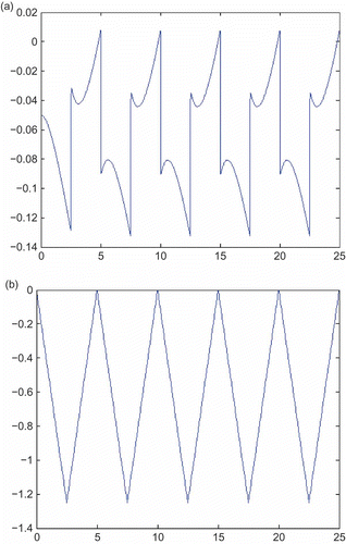
For the parameter values given for Equation (16)(16), a value of T = 0.01 s is appropriate. The specification for the desired output, y(t), is chosen to be an ideal saw-tooth type of signal starting at y = 0 at time t = 0 s with a period of 5 s. Figure 3(a) shows the result of an inverse simulation for this model using the transfer function manipulation, signal generation and linear system simulation facilities of the MATLAB Control Systems Toolbox [17]. The value of time constant T used in this case was 0.01 s. Figure 3(b) shows the result of a test in which the signal resulting from the inverse simulation shown in Figure 3(a) is applied as input to the simulation model for G(s). It can be seen that the output of the forward model G(s) found in this way matches the specification given above. More detailed examination shows that the maximum error is of the order of 0.006, confirming the accuracy of this inverse simulation procedure. This maximum error is reduced to 0.0006 if the time constant T of the ‘propering’ component is reduced to 0.001 s.

Figure 3. (a) Input signal required to give the specified repeated ramp output, as generated by inverse simulation. (b) Output of the model when subjected to input found from inverse simulation.

As shown in the block diagram of Figure 2, the sensitivity of the variable u(t) in the inverse model to variation of the parameter a may be obtained by applying the signal u(t) to a simulation representing the sensitivity model of Equation (17)(17). The resulting sensitivity function is shown in Figure 4(a). Figure 4(b) shows the same sensitivity function determined by parameter perturbation for a 10% change in the parameter a. Although the forms of the sensitivity functions are the same by these two methods, numerical values for the sensitivity function found by parameter perturbation differ slightly from those determined by means of the sensitivity model. It should be noted that if the parameter change is reduced to 1% the result obtained by the perturbation methods becomes almost identical to that found from the sensitivity model.

Figure 4. (a) Sensitivity function determined from the sensitivity model. (b) Sensitivity function determined using the parameter perturbation approach for a change of 10% in the parameter a.

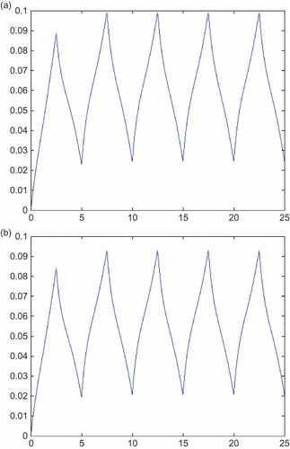
Results obtained using the sensitivity model approach for the parameters b and c are shown in Figures 5 and 6. In both the cases, results found using the parameter perturbation method for 10% changes of each parameter are identical, within the width of the lines in the relevant plots, to those found using the sensitivity model.

Figure 5. Sensitivity function determined from the sensitivity model.

Figure 6. Sensitivity function determined from the sensitivity model.

3.1.2. The MIMO case

Inversion of a matrix of transfer functions representing a MIMO system requires checks to be made to establish the number of eigenvalues (poles) and transmission zeros and to add propering poles (if necessary) to each transfer function within the matrix in order to make the inverse model realizable. The process of inversion for each transfer function and the generation of the associated sensitivity model involves use of the procedure applied in the SISO case. Buchholz and von Grünhagen [4] present an approach for this procedure based on the use of the MATLAB Symbolic Math Toolbox [18] but the process can also be carried out manually.

Example:

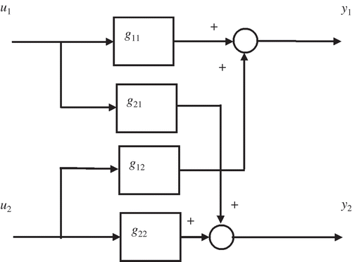
The example considered is one that has been used by O'Reilly and Leithead [19] and involves a two-input two-output model adapted from a system considered previously by Rosenbrock [20]. The structure of the system is shown in Figure 7 and it may be seen that the model has four pathways between the inputs and outputs, described by transfer functions g ₁₁(s), g ₂₂(s), g ₁₂(s) and g ₂₁(s). The individual transfer functions are as follows:

(22)

Figure 7. Block diagram of two-input two-output model considered in the example.

The inverse model found using the inv function within the MATLAB Control System Toolbox [17] (which allows inversion of linear time-invariant transfer matrices) involves the following inverse transfer function matrix:

(23)

Direct inversion of this model requires the addition of factors to each of the transfer functions to make this inverse model realizable, but the process is straightforward in principle. Sensitivity functions for each of the transfer functions in the inverse simulation model may be obtained using the procedure applied in the SISO case, as described above.

3.2. Sensitivity models for inverse simulations derived using feedback principles

The feedback approach to inverse simulation ([4,10]) can be applied to both SISO and MIMO models.

3.2.1. The SISO case

Consider the feedback structure of Figure 8 with a linear SISO model G(s), leading to an inverse solution w(s) through application of the approach described in [10]. The sensitivity of the signal w(s), which represents the inverse solution, for a specific parameter q_i is as follows:

(24)

Figure 8. Block diagram of sensitivity model for determination of the inverse sensitivity for j parameters of a SISO linear model G(s) using the sensitivity model approach.

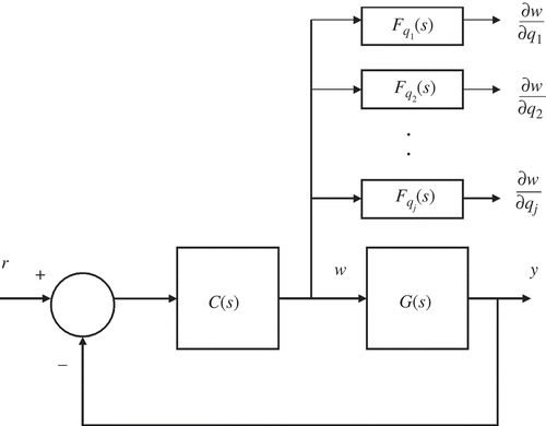
The sensitivity of the inverse solution can therefore be found by passing the signal w through a block having transfer function

(25)

This transfer function depends entirely on the characteristics of the forward model G(s) and is found easily using analytical methods. It provides the same form of filter as in Equation (13)(13), but as the numerator and denominator of the closed-loop system transfer function are always of the same order as the denominator of the open-loop transfer function there is no need for an additional propering element. A different transfer function applies for each parameter of the model and the sensitivity functions for a number of parameters can be found simultaneously using a number of parallel blocks of this kind, as shown in Figure 8. A similar approach can, in principle, be used for the case of an inverse simulation involving a non-linear model. However, the determination of the sensitivity model F is more complicated and it may be preferable to apply a finite difference approach in such cases.

Example:

Consider the linear SISO system in Section 3.1. The transfer function of the model has the form:

(26)

and it follows from the discussion above that

(27)

(28)

(29)

(30)

In all of these expressions, the inverse solution U(s) is found from the signal W(s) in the feedback system. The filters required are therefore identical in form to those found above using the transfer function inversion approach. This is to be expected as the only difference is the way in which the inverse is generated, and the sensitivity analysis is essentially the same in the two cases.

Figure 9 shows the root locus diagram for the feedback system that provides the basis of this inverse simulation and analysis can be used to show that, for a gain factor of 1000, one closed-loop system pole lies very close to the position of the zero of the forward model G(s) at s = −1, whereas the other pole lies on the negative real axis at about s = −10,000. Therefore, an inverse simulation result obtained using this value of gain factor should be almost perfect.

Figure 9. Root locus diagram, for the feedback system used for the inverse simulation of the transfer function G(s).

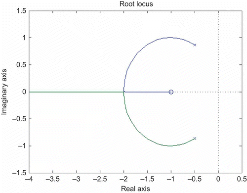
For the same parameter values (K = 10, a = 1, b = 1 and c = 1) and the desired output used in the example of Section 3.1 with a value of feedback gain of 1000, the inverse solution is indistinguishable from that found previously using the approximate transfer function inversion method and shown in Figure 3(a). As the sensitivity models have the same structure and parameters as in the approximate transfer function approach, sensitivity functions found by the feedback method of inversion are, in theory, the same as those obtained through approximate transfer function inversion and, for the cases considered, were found to be identical to those in Figures 4(a)–6.

The advantage of the feedback approach over the use of the approximate transfer function inversion method is that it can be applied to non-linear models, as well as to linear descriptions. In addition, the introduction of feedback means that there is no issue of realizability so that no additional poles have to be introduced. The positions of the poles of the closed-loop system do have to be found and checks must be carried out to establish that the feedback system can provide an acceptable approximation to the inverse model. In the case of non-linear models, these tests may involve applying the input found from inverse simulation to the forward simulation model and establishing the magnitude of the model output error, using an appropriate measure, when the output is compared with the desired output. There are, of course, potential problems of instability within the closed-loop system and obvious limitations in the cases where the transfer function to be inverted is of non-minimum phase form with one or more zeros in the right half plane.

It should be noted that in the non-linear case the sensitivity model becomes significantly more complicated and the time required for development of the sensitivity model and for implementation in the simulation can become significant. In such cases, the process of obtaining sensitivity information using the parameter perturbation approach may well be more attractive, although useful insight about the properties of the sensitivity functions is lost.

3.3.2. The MIMO case

Inverse simulation for MIMO models can also be carried out using the feedback technique. This can best be introduced by considering the general two-input two-output model used already in the example given in Section 3.1. Figure 10 shows the block diagram for the feedback structure required for inverse simulation in this case.

Figure 10. General form of block diagram for inverse simulation of a two-input two-output model. The signals w ₁ and w ₂ represent the inverse solutions.

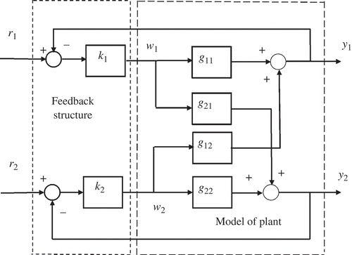
As would be expected there are two reference inputs and two feedback pathways. As in the SISO case, the inverse solutions are found from the signals at the inputs to the model block G(s). These are shown as the signals at the outputs of the controller blocks k ₁ and k ₂ in Figure 10.

The cross-coupling through the blocks g ₁₂(s) and g ₂₁(s) in this model can be represented using a modified structure that forms the basis of the ‘individual channel’ approach, which has been developed for analysis and design of MIMO closed-loop systems [19]. In the Individual Channel Analysis and Design (ICAD) methodology, the MIMO structure of the system may be translated into two SISO feedback loops while preserving loop interactions. Figures 11 and 12 show block diagrams of two channels, which, taken together, are equivalent to the structure of Figure 10 [19].

Figure 11. Structure of Channel C₁, which represents a single-input single-output model for the system-linking reference input r ₁ and output y ₁ with an additional disturbance pathway representing the effect of reference input r ₂. For output y ₁, this is equivalent to the structure of the two-input two-output diagram of Figure 10.

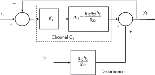
Figure 12. Structure of Channel C₂, which represents a single-input single-output model for the system linking reference input r ₂ and output y ₂ with an additional disturbance pathway representing the effect of reference input r ₁. For output y ₂, this is equivalent to the structure of the two-input two-output diagram of Figure 10.

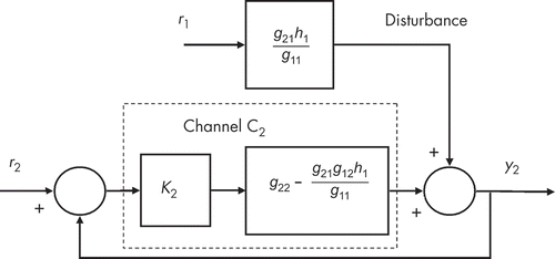
The coupling pathways between Channels C₁ and C₂ appear now as disturbance inputs. The quantities h ₁ and h ₂ in these diagrams are defined as follows:

(31)

(32)

The use of the concept of individual channels allows use of the feedback approach to the development of sensitivity models for the inverse simulation. For simplicity in interpreting results it is useful to investigate parameter sensitivities for each of the inputs in turn. If the reference input r ₂ is 0 so that we are defining an output y ₁ only, the signal w ₁ has the form

(33)

Similarly, if the reference input r ₁ is 0 so that we are defining an output y₂ only, the signal w ₂ has the form

(34)

Because of the cross-coupling within this model, both the inputs w ₁ and w ₂ depend on all four of the transfer functions of this two-input two-output model. The sensitivity functions for these input signals can be obtained by partial differentiation for any parameter of any of these transfer functions. For example, if the parameter of interest appears only in the transfer function g ₁₁ it can be shown by simple manipulation that:

(35)

and, similarly, if q is a parameter within the transfer function g ₂₂ then

(36)

Equivalent expressions can be derived for the cases involving parameters of the other two transfer functions within the model G(s). These all involve applying the signals w ₁ and w ₂ to sensitivity models, which have a relatively simple form. As in the SISO case, sensitivity functions may be obtained simultaneously through the use of a number of sensitivity models in parallel, each coupled to the inverse simulation outputs w ₁ and w ₂.

Example:

The model considered is the two-input two-output description used in the MIMO example given in Section 3.1. The individual transfer functions are as follows:

(37)

With a feedback structure of the form shown in Figure 10 and appropriately high values of gain in the blocks labelled k ₁ and k ₂, the two reference inputs r ₁ and r ₂ provide the two desired outputs y ₁ and y ₂ and the inverse solutions are the two signals at the input to the plant model. The two reference inputs are chosen to be sinusoidal in form with r ₁ = sin (2πf ₁ t) and r ₂ = sin (2πf ₂ t), where f ₁ = 0.25 Hz and f ₂ = 0.5 Hz. Figures 13 and 14 show inverse simulation results for this set of desired outputs in terms of the signals at the two plant model inputs (w ₁(t) and w ₂(t)), obtained using gain factors k ₁ = k ₂ =1000.

Figure 13. Inverse simulation results for the two-input two-output example for input w ₁(t).

Figure 14. Inverse simulation results for the two-input two-output example for input w ₂(t).

Application of the inputs shown in Figures 13 and 14 to the forward model of the system G(s) gives results that reproduce, almost exactly, the desired sinusoids. The maximum output error in both cases is of the order of 3 × 10⁻³, which is small compared with the maximum output values of unity. The use of larger values of the feedback loop gain factors would reduce these errors but would increase the stiffness of the inverse simulation.

Sensitivity analysis in this case follows the procedure outlined above, leading to expressions of the type given in Equations (35)(35) and (36(36)). For example, if the parameter of interest is in the transfer function g ₁₁(s) (which has the general form with c = v =1), the sensitivity function equivalent to result from Equation (39)(39) has the form

(38)

Implementation of the sensitivity model of Equation (38(38)) shows that the filter applied to the inverse solution given by the signal w ₁ has a simple structure involving two poles and one zero and presents no problems in terms of implementation. It is of interest to note one of these poles is not a pole of any of the plant transfer functions.

4. Case study: a linearized model for diving motion of an unmanned underwater vehicle

The linearized dynamics describing diving motion of an underwater vehicle model [21,22] involves a third-order model described by the following set of first-order equations:

(39)

The state variables q, θ and z are the pitch rate, pitch angle and vertical displacement, respectively, and δ _s is the stern plate deflection. The parameters M_q , and M _δ are hydrodynamic coefficients, I_y is the moment of inertia of the vehicle for pitching motion, W is the weight of the vehicle, z _G − z _B is the vertical distance between the centre of gravity and the centre of buoyancy and u ₀ is the forward speed of the vehicle. The stern plane has actuator limits, which restrict the control surface deflection to ±25°. Thus, if actuator signals are applied, which correspond to values of surface deflection greater than this, the surface displacement reaches a saturation limit at +25° or −25°.

In simplified form, these equations may be written as

(40)

It may be seen from Equations (39)(3) and (40) that the parameter a ₁₁ depends directly on M_q and inversely on I_y and . Similarly, the parameter a ₁₂ depends directly on W, z _G and z _B, and inversely on I_y and whereas b ₁ depends directly on M _δ and inversely on I_y and . The only other significant parameter of Equation (40)(4) is a ₃₂, which is –u ₀ and thus depends directly on the forward speed of the vehicle.

The transfer functions relating the pitch rate, q, pitch angle, θ, and vertical displacement, z, to the stern-plane deflection, δ_s, are as follows:

(41)

(42)

(43)

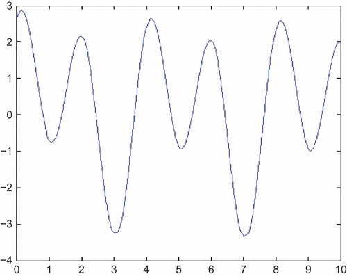
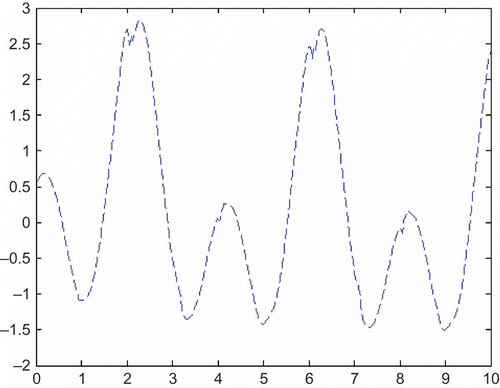
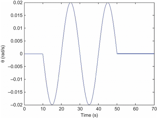
For typical operating conditions, the parameters are a ₁₁ = −0.7, a ₁₂ = −0.3, u ₀ = 1.832 m/s and b ₁ = 0.035. Design of a feedback system for inverse simulation for a defined pitch-rate time history is very straightforward and can be achieved with proportional control using high-gain feedback, as in the SISO example in this section. If the trajectory is defined in terms of the pitch angle, θ, or vertical displacement, z, simple root locus analysis shows that proportional control is no longer appropriate because there are additional closed-loop poles present, which are located at points in the s-plane that are too close to the poles and zeros of the model. In this case, a useful alternative involves design of a feedback system for inverse simulation using proportional plus rate feedback. Using feedback of 6000 from the pitch rate variable, it can be shown that for values of gain factor in the pitch-angle feedback loop of 3 × 10⁵ the inverse simulation model has zeros at the positions of the two poles of the forward model (s = −0.35 ± j0.42) and two additional poles that lie far from these points (at approximately s = −100 rad/s). Results for a demanded sinusoidal form of pitch-angle trajectory, with these gain factors in the feedback loops, are shown in Figure 15.

Figure 15. Stern-plane input signal found from inverse simulation for required trajectory involving a demanded sinusoidal change of pitch angle for gains of 300,000 in the feedback loop involving θ and 6000 in the feedback loop involving q.

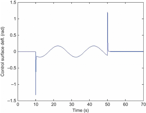
It can be seen from the result that in order to generate the demanded response in terms of the pitch angle, θ, the maximum stern-plane deflections (approximately ±1.3 rad) would be very much larger than the upper limit of the actuator and control surface deflection (25°). Thus, the pattern of input required for this demanded maneuver could not be applied and the requirement would have to be modified or, if it was essential to be able to follow this specific pattern of pitch change, fundamental re-design of the control surface and actuator would be necessary.

Note that application of the stern-plane deflection signal of Figure 15 to the forward model of the unmanned underwater vehicle (UUV) (without control surface limits) gives an output that is almost identical to the required sinusoid, as shown in Figure 16. This demonstrates satisfactorily that the input generated using inverse simulation produces the demanded output when applied to the given model.

Figure 16. Pitch-angle record found from application of stern-plane deflection signal of Figure 15 to the forward model of the UUV in the absence of control surface limits.

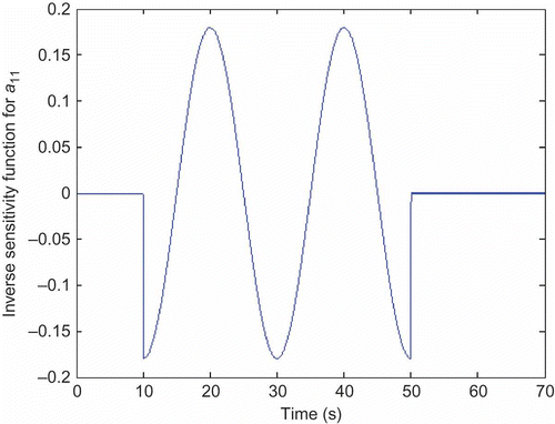
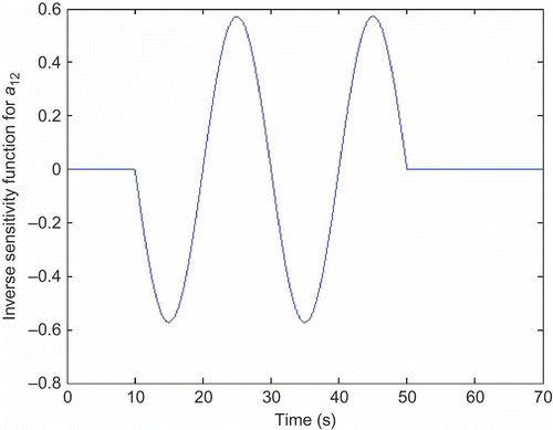
Application of the technique outlined above for determination of the sensitivity of the inverse solution to parameters of the given model, such as a _11, a ₁₂ and b ₁, involves the application of appropriate filters F_qi (s) to the simulated signal, which represents the required control surface input δ_s(t).

In the case of the parameter a ₁₁, the filter can be shown to have the transfer function

(44)

For the parameter a ₁₂, the transfer function has the form

(45)

and for b ₁, the transfer function has the form

(46)

Results obtained using this method of sensitivity analysis for the inverse simulation model are shown in Figures 17 and 18. It can be seen that the parameter sensitivity function is dominated by a cosine function of amplitude approximately 0.18 with a frequency that is the same as that of the required pitch change signal. The sensitivity function is sinusoidal in form and identical in frequency to that for a ₁₁ with a peak value of approximately 0.58. As would be expected from the form of the filters given above, the sensitivity function for a ₁₁ is shifted in phase compared with that for a ₁₂ by 90° and these two parameters therefore have the greatest influence on the stern-plane deflection signal at different times. The influence of each of the parameters can be compared quantitatively using the relative sensitivity measures and . On that basis it may be shown that the stern-plane defection signal sensitivities for parameters a ₁₁ and a ₁₂ have similar magnitudes. It has already been noted, from Equations (39)(3) and (40), that the coefficient a ₁₁ is directly proportional to the parameter M_q , which is one of the hydrodynamic coefficients of the underwater vehicle model, whereas the coefficient a ₁₂ is directly proportional to the parameter W (the weight of the vehicle) and to (z _G − z _B), which is the vertical distance between the centre of gravity and the centre of buoyancy. The sensitivity functions thus show that a change in the weight of the vehicle, or of the position of the centre of gravity relative to the centre of buoyancy, has no influence on the initial and final transients in the plot of control surface deflection (Figure 15). As both the coefficients a ₁₁ and a ₁₂ involve the factor 1/(I_y  − ), it is clear that the parameter is the quantity that has the most influence on the initial and final transients in the stern-plane deflection records. Sensitivity information of this kind is potentially useful when considering actuator performance limits and when carrying out control system optimization studies.

Figure 17. Sensitivity function found from sensitivity model for parameter a ₁₁.

Figure 18. Sensitivity function found from sensitivity model for parameter a ₁₂.

For the parameter b ₁, the form of the filter for generation of the sensitivity is very simple and involves only a gain factor −. It is clear, therefore, that the sensitivity function for this parameter has a shape that is identical to the pattern of control surface deflection shown in Figure 15 and that this parameter therefore influences all parts of the control surface deflection record in the same way.

It should be noted that sensitivity functions for the parameters found directly from the inverse simulation results using a perturbation approach give closely similar results. For example, perturbation results for the sensitivity functions and for 10% changes in parameter values are almost identical to those shown in Figures 17 and 18.

Similar information on inverse sensitivity of the control input δ _s to variation of the model parameters could be derived in the same way for demanded changes of the vertical displacement z. In this case, the feedback pathway of Figure 8 would involve the variable z and it can be shown, from Equation (43)(43), that the sensitivity filters required for parameters a ₁₁, a ₁₂ and b ₁ would be identical to those given in 44–46). The sensitivity filter for parameter a ₃₂ can also be shown to have a transfer function , which is equivalent to . It can thus be seen that for variations in depth the sensitivity function depends inversely on the forward speed of the vehicle. Thus, as would be expected from physical reasoning, this shows that at low forward speeds of the vehicle larger stern-plane deflections are required to produce a given change of vertical displacement than at higher forward speeds.

5. Discussion and conclusions

Inverse simulation techniques provide information about the inputs that allow the output of a given system to match specific forms of required response. This could involve an aircraft, helicopter or marine vehicle performing a specified maneuver or the inputs that ensure that a robotic arm follows a given trajectory.

Inverse simulation methods are especially relevant for applications in which actuator performance is important and where design decisions have to be made about the size and shape of control surfaces linked to actuators or to engines, motors and other drive-train components. For example, if an inverse simulation of a vehicle or robot shows that no inputs can be found that allow a specified maneuver to be performed, changes must be made to the required maneuver or within the hardware or software of the system itself. Within this design process, knowledge of the sensitivity of inverse solutions to variation of parameters of a model can be of considerable importance, as introduced in Section 1.

The methods of inverse simulation discussed in this article involve approximate transfer function inversion (which is restricted to linear models) and also a feedback approach that is applicable to both linear and non-linear descriptions. This feedback-based method of inverse simulation has been described and applied in a recent article [10], and it is believed that, for many applications, it can have computational advantages compared with more established iterative methods of inverse simulation (e.g. [1,2]).

In addition to design applications, parameter sensitivity information can also be very useful within the model validation process when comparing model behaviour with experimental test records for the same maneuver. This issue has been touched upon by Thomson and Bradley [1] who state that ‘ … despite the benefits, established parameter estimation methods such as the output error method have not been applied to the inverse problem’. This is an interesting area for future research and one for which access to parameter sensitivity information has potential importance, especially in the context of methods of system identification that involve the use of sensitivity concepts, such as those proposed by Knudsen [23,24]. The reason for incorporating parameter sensitivity information within the identification process is that estimation of any given parameter requires a cost function that is sensitive to that parameter. The most sensitive parameters are likely to be those that are estimated most accurately. Knowledge of parameter sensitivities is thus very useful for assessing identification results.

For linear models, the sensitivity model approach to parameter sensitivity analysis can be applied both for inverse simulation responses generated using approximate transfer function inversion and also for inverse solutions found by use of the feedback approach. In all linear cases, the sensitivity model appears to have advantages over parameter perturbation methods in terms of additional physical insight and also, in some cases, computational efficiency. As indicated in Section 2.1, the estimation of sensitivity functions through application of the method of repeated solutions is a purely numerical procedure and has the disadvantage of requiring the difference to be taken between two simulation solutions that, inevitably, are very similar because the parameter perturbation must, by definition, be small. As shown in Sections 3.1, 3.2 and 4, the additional insight that is gained through use of sensitivity models is especially evident in the case of inverse simulation for a linearized model. In such cases, the sensitivity functions are derived from transfer functions where knowledge of the poles and zeros can provide valuable physical understanding that can be of direct use in the investigation of sensitivity issues. An additional point of interest, which is mentioned in Section 3.2.1, is that the structures of the sensitivity models are the same for inverse simulations based on the approximate transfer function inversion method and for inverse simulations involving use of the feedback method.

In the case of non-linear models the sensitivity model can be complex and sensitivity analysis through parameter perturbation may be preferred. However, in such cases, physical insight may be obtained through additional sensitivity analysis using a linearized version of the model for a specific operating point. It is also possible to generate approximate sensitivity information in the non-linear case by combining the use of a linearized sensitivity model for an appropriate operating condition with an inverse response obtained from a non-linear inverse simulation, including solutions found using iterative methods of inverse simulation, such as those discussed in [1] and [2]. As with all investigations based on linear models, it is clear that caution must be exercised in interpreting results obtained from these linearized sensitivity models but the physical insight that this process provides may well be useful.

Acknowledgements

The author thanks the US Office of Naval Research for the funding that supports some aspects of the work described in this article through awards to California State University, Chico, and associated sub-contracts placed at the University of Glasgow by California State University. The author also thanks Dr R.E. Crosbie of the Department of Electrical and Computer Engineering, California State University, Chico, for the support and continuing interest that he has shown in this research. The author also thanks the three anonymous reviewers of this article for helpful suggestions, which have been included in the revised version of the article.

References

- Thomson , D. and Bradley , R. 2006 . Inverse simulation as a tool for flight dynamics research – Principles and applications . Prog. Aerosp. Sci. , 42 : 174 – 210 .
- Hess , R.A. , Gao , C. and Wang , S.H. 1991 . A generalized technique for inverse simulation applied to aircraft maneuvers . AIAA J. Guid. Control Dyn. , 14 ( 5 ) : 920 – 926 .
- Fröberg , A. 2005 . Extending the inverse vehicle propulsion simulation concept – to improve simulation performance , Sweden : Department of Electrical Engineering, Linköpings universitet . Linköping Studies in Science and Technology, Thesis No. 1181
- Buchholz , J.J. and von Grünhagen , W. September 2004 . Inversion impossible? , September , Germany : Tech. Rep., University of Applied Sciences Bremen .
- Isidori , I. 1989 . Nonlinear Control Systems: An Introduction , 2nd , Berlin : Springer .
- Slotine , J.-J.E. and Li , W. 1991 . Applied Nonlinear Control , Englewood Cliffs, NJ : Prentice Hall .
- Hunt , L.R. and Meyer , G. 1997 . Stable inversion for nonlinear systems . Automatica , 33 ( 8 ) : 1549 – 1554 .
- Zou , Q. and Devasia , S. 2007 . Preview-based inversion of nonlinear nonminimum-phase systems: VTOL example . Automatica , 43 ( 1 ) : 117 – 127 .
- Lu , L. , Murray-Smith , D.J. and Thomson , D.G. 2008 . Issues of numerical accuracy and stability in inverse simulation . Simul. Model. Pract. Theory , 16 : 1350 – 1364 .
- Murray-Smith , D.J. 2011 . Feedback methods for inverse simulation of dynamic models for engineering system applications . Math. Comput. Model. Dyn. Syst. , 17 ( 5 ) : 515 – 541 .
- Tomović , R. 1963 . Sensitivity Analysis of Dynamic Systems , New York : McGraw-Hill .
- Frank , P.M. 1978 . An Introduction to System Sensitivity Theory , London : Academic Press .
- Tomović , R. and Vukobratović , M. 1972 . General Sensitivity Theory , New York : American Elsevier .
- Kokotović , P.V. 1964 . Method of sensitivity points in the investigation and optimization of linear control systems . Autom. Remote Control , 25 : 1670 – 1676 .
- Rosenwasser , E. and Yusupov , R. 2000 . Sensitivity of Automatic Control Systems , Boca Raton, FL : CRC Press .
- Wilkie , D.F. and Perkins , W.R. 1969 . Generation of sensitivity functions for linear systems using low-order models . IEEE Trans. Autom. Control , 14 : 123 – 129 .
- MathWorks, Documentation, Control Systems Toolbox™. http://www.mathworks.co.uk/help/toolbox/control/ (http://www.mathworks.co.uk/help/toolbox/control/) (Accessed: 4 February 2012 ).
- MathWorks, User's Guide, Symbolic Math Toolbox™ . http://www.mathworks.co.uk/help/toolbox/symbolic/bqs6eo_.html (http://www.mathworks.co.uk/help/toolbox/symbolic/bqs6eo_.html) (Accessed: 4 February 2012 ).
- ’Reilly , J. O and Leithead , W.E. 1991 . Multivariable control by ‘individual channel design’ . Int. J. Control , 54 ( 1 ) : 1 – 46 .
- Rosenbrock , H.H. On the design of linear multivariable control systems . Proceedings of the 3rd IFAC Congress . 1966 , London . Vol. 1 , London : Institution of Mechanical Engineers . Book 1, Paper 1A
- Healey , A.J. and Lienard , D. 1993 . Multivariable sliding-mode control for autonomous diving and steering of unmanned underwater vehicles . IEEE J. Ocean Eng. , 18 ( 3 ) : 327 – 339 .
- Fossen , T.I. 1995 . Guidance and Control of Ocean Vehicles , Chichester : Wiley .
- Knudsen , M. 2006 . Experimental modelling of dynamic systems: an educational approach . IEEE Trans. Edu. , 49 ( 1 ) : 29 – 38 .
- M. Knudsen, Senstools. www.control.auc.dk/˜mk/public_html/ExpMod (http://www.control.auc.dk/~mk/public_html/ExpMod) (Accessed: 7 June 2012 ).