Incremental optimal process excitation for online system identification based on evolving local model networks

Abstract

In this paper, a methodology for the generation of optimal input signals for incremental data-based modelling of nonlinear static and dynamic systems is presented. For this purpose, an online strategy consisting of an evolving model and an iterative finite horizon input optimization in parallel to the ongoing experiment is pursued. Such an integrated methodology is methodically very efficient since the experiment is only conducted until the desired model quality is obtained. For the process excitation, the compliance with system input and output limits is of great importance. Especially for nonlinear dynamic systems, the compliance with output constraints is challenging since the current input has an impact on all forthcoming outputs. The generation of optimal inputs is based on the iterative optimization of the Fisher information matrix of the current process model subject to input and output constraints. For the identification, an evolving local model network is used that can cope with a growing amount of data. To this end, the parameter adaptation and the automated structure evolution are characteristic of the evolving local model network. The effectiveness of the proposed method is demonstrated on two typical automotive application examples. First, a stationary smoke model of a diesel engine and second, a dynamic exhaust temperature model are identified by use of optimal process excitation.

Keywords:

• online design of experiments
• online training
• nonlinear systems
• neural networks
• local model networks
• system identification

1. Introduction

1.1. Motivation

In nonlinear system identification, informative experimental data are required in order to build proper process models [1]. Therefore, it is necessary that the data excite the necessary process dynamics as well as the system nonlinearities. With increasing complexity of the underlying system, the information demand on the excitation data increases which usually leads to more time-consuming experiments. But for many processes, the duration of the experimental run is limited due to the high effort involved in the execution of the experiment. Therefore, methods for the design of experiments (DoE) are required that gain as much information as possible from the underlying system in minimum time. For this purpose, model-based DoE approaches have been developed that use a reference process model in order to optimize excitation signals (e.g. [2]). In this context, the Fisher information matrix based on the reference model is used to assess the information content in order to generate optimal excitation signals for the estimation of parameters with minimal variance, cf. [3].

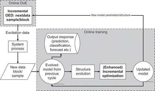
There are two possible configurations for model-based design of experiments. First, the experiment design can be generated offline and then be applied to the system. Second, the so-called online method is based on an incremental generation of new experiments in combination with evolving modelling of the underlying process, e.g. [4]. In Figure 1, the workflow for the online DoE and the modelling strategy is depicted. In every sampling period, an optimal input sequence is generated by use of the current state of the evolving model but only the most recent input is applied to the system. The obtained data are used to update the model and based on the current model, new experiments are generated. This procedure of incremental experiment design and modelling is repeated until the quality of the evolving model achieves a satisfying performance.

Figure 1. Generation of an optimal experiment design (OED) in an online procedure based on an evolving model.

1.1.1. Potential of incremental experiment design for online modelling

1. Since the process model is trained online in parallel to the running experiment, there is the possibility to continuously assess its quality and if a satisfactory result is achieved, the identification procedure is stopped. In contrast to offline identification, new experiments do not have to be carried out once the model quality is satisfactory.

2. The design of future experiments builds on the current data obtained from the experiment and on the current state of the evolving model. If the running process alters or if new insight is obtained, the incremental generation of new inputs is able to adapt to these changes. This gives an additional benefit over offline-generated experiment designs that are not able to respond to new information provided by the measured data.

3. The compliance with system limits during the experimental run is very important in order to protect the plant against damage. The limits themselves are known (e.g. maximum exhaust gas temperature of engines ). But the effect of inputs on output limit violations is not known. The evolving model gives the opportunity to predict future system limit violations. These predictions are considered in the online experiment design so that the resulting excitation signal complies with input and output constraints.

1.1.2. Challenges of incremental experiment design for online modelling

1. An evolving model is required that is able to adapt its parameters and structure to a growing amount of data. This model has to have the flexibility to increase its complexity if new nonlinearities are revealed by the experiment.

2. In every sampling period, the design of future experiments is based on the currently available data and the most recent state of the evolving model. Therefore, a recursive optimization scheme of future system inputs is required that is targeted to estimate the parameters of the evolving model with minimal variance.

3. The compliance with system limits is crucial in order to provide stable and secure operating conditions of the underlying plant. Therefore, system constraints have to be considered in the experimental design. Especially for nonlinear dynamic systems, the compliance with output constraints is challenging since every input influences the evolution of all future system outputs.

4. The incremental DoE and the identification are executed in parallel to the running experiment. As a consequence, the experiment design and modelling procedure has to cope with an increasing amount of data in real time.

1.2. Proposed concepts

In this paper, a method for incremental experiment design for the online identification of nonlinear static and nonlinear dynamic systems is proposed. An evolving local model network (LMN) [5] is applied for modelling as well as optimization of future experiments. For this purpose, a recursive input optimization scheme is presented that is targeted to optimize a scalar criterion of the Fisher information matrix of the evolving LMN. In every sampling interval, a feasible solution for a finite horizon of future system inputs is generated that is subject to system input and output constraints.

This paper is organized as follows: In Section 2, the evolving LMN is reviewed and in Section 3, the method for the constrained iterative generation of optimal input signals is presented. In Section 4, the effectiveness of the proposed method is demonstrated on two typical application examples of the automotive industry. Finally, in Section 5, the conclusion is given.

2. Evolving local model network

2.1. Model architecture

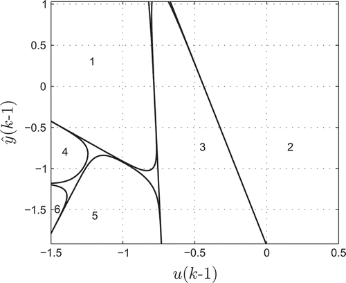
In this paper, an evolving LMN is used that is based on a LMN with an incremental model tree, cf. [6]. The basic concept of the LMN architecture is to distinguish between the input space and the partition space. The input space contains all physical quantities that are needed to describe the process forming the regressor vector . However, the partition space comprises all physical quantities that are necessary to describe the system nonlinearities. Prior knowledge on the true nature of the underlying process is included into the model by proper choice of the partition space that might also drastically reduce the model complexity. The partition space is split into subdomains that are described by local models (LMs) that are linear in their parameters. The transition from one LM to a neighbouring LM is determined by a smooth activation function. Each LM has a certain area of validity defined by the validity function . The subscript i indicates one LM. In Figure 2, the validity functions for a two-dimensional input space for a model consisting of six LMs is depicted. The applied evolving LMN is able to make an axis-oblique partitioning. The estimated output of the ith LM is given by the scalar product of the regressor vector and the parameter vector of the ith LM :

(1)

Figure 2. Contour lines of the validity functions of a local model network with six local models. The partition space is spanned by and .

The global parameter vector comprises the parameters of all LMs.

(2)

The global model output is obtained by a weighted aggregation of all LM outputs and the according validity functions.

(3)

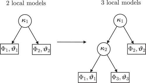
A characteristic of the evolving LMN is its structure that can be incrementally enhanced. For this purpose, the computation of the validity functions is based on a hierarchical model tree. In Figure 3, the transition from two to three LMs is depicted by means of the hierarchical model trees. A LM is represented by the free ends of the tree with the validity functions and the parameters . Each node represents a split in the partition space into two subdomains. The sequential, partitioning strategy follows the tree from the top to the bottom. In this case, the initial split of the partition space is indicated by leading to the validity functions and . Then the LM number one is replaced by two new LMs () with new validity functions and . Whenever the number of LMs is increased, the number of parameters is augmented. Evolving LMNs are able to represent both nonlinear static and nonlinear dynamic systems. In general, the evolving LMN is characterized by the ability to adapt its structure as well as its parameters to a data stream and to a packet of data, respectively (cf. [7]). In this paper, an evolving LMN is used that combines the incremental structure of the LMN with an online training strategy that decides, by means of a statistical criterion whether the structure should be enhanced (i.e. number of LMs is increased), cf. [5]. The initialization of new parameters of the evolving LMN does not depend on random numbers. This increases the repeatability and the robustness, which is a very important prerequisite for online applications. Model architectures that depend on random initializations such as multilayer perceptron networks (MLP) might require the computation of several models before a proper result is achieved, which can cause a very high computational effort, cf. [8].

Figure 3. Illustration of the hierarchical model trees for two and three local models.

The evolving LMN gives the opportunity to incorporate physical knowledge about the true system under investigation. Thereby, the complexity of the model can be reduced and the computational speed is increased. An additional benefit arises from the structure of the evolving LMN that gives the possibility to physically interpret its parameters, cf. [9].

2.2. Online training strategy

The evolving LMN combines the incremental model structure with an online parameter estimation algorithm that decides when the model has to grow. This decision is made upon a statistical criterion based on the current data in order to automatically detect when is it reasonable to increase the number of LMs. For this purpose, the distribution of the residuum variance of the output estimates is the subject of investigation. Under the assumption that the variance of the model error of the ith LM is described by a distribution, the confidence interval for a certain error probability is obtained:

(4)

The quantity indicates the statistical degrees of freedom and represents the estimated variance. With increasing number of observations, the confidence interval decreases. If the estimated variance of a local output exceeds the given confidence interval, then this very LM is split. In this context, the error probability is a regularization parameter. For a small , the confidence interval is larger which leads to a smaller number of LMs and a more robust model while reducing the accuracy. If is increased, a greater number of LMs is achieved which increases not only the model accuracy but also the risk of overfitting.

Apart from the splitting rule for the worst LM, the online algorithm optimizes its parameters with every new incoming sample. For this purpose, the split in the latest node of the model tree is optimized by minimizing the quadratic model error of the two associated LMs. Then all the parameters of all LMs are updated.

If the algorithm decides that the model is extended, the partitioning weights describing where the worst LM is divided are initialized. This initialization is based on the weighted mean and the covariance matrix of the observations within this LM. Since the initialization does not depend on random numbers, the robustness of the training algorithm is increased.

3. Online model-based design of experiments

Online model-based design of experiments is a method for the incremental generation of optimal input data for continuous and efficient on-the-fly process excitation. For this purpose, the available data and the current state of the evolving model are used to optimize the information content of future process excitation. Due to the fact that the model adapts its parameters and structure to the incoming data stream, the generation of a finite sequence of future system inputs evolves with every new sample.

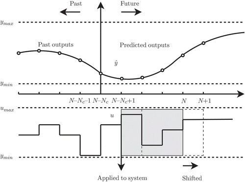
In Figure 4, the principle of online experiment design is depicted. Based on the current model, an optimal future input sequence, , is generated but only the first sample of this sequence, , is applied to the system. When the next sample period arrives, the most recent measurement of the system output is used to update the process model. The excitation signal grows by one sample, , and the optimization horizon is shifted forward () in order to generate a new sequence of future inputs. The procedure is repeated until a proper model is obtained.

Figure 4. Online optimization of future system inputs under constraints.

This approach is very similar to the receding horizon principle for model predictive control (MPC), cf. [10]. MPC is also targeted to incrementally generate an optimal input sequence for optimal process control. For this reason, a cost function that is based on the setpoint trajectory is subject to minimization. As opposed to MPC, in online DoE, the cost function is based on a scalar criterion of the Fisher information matrix.

The process excitation has to comply with system limits in order to provide stable and secure operational conditions. Therefore, the optimization of the Fisher information matrix has to comply with system input and output constraints. In light of these considerations, the following critical issues arise for online model-based design of experiments:

• Regarding the receding horizon principle, the Fisher information matrix has to be optimized recursively.

• The optimization of the Fisher information matrix is subject to constraints. The obtained input sequence has to be feasible in terms of input and output constraints.

• According to the definition of the Fisher information matrix (see Section 3.1), the number of parameters determines its dimension. Therefore, every time the number of LMs is increased, the Fisher information matrix grows in dimension.

• Design criteria that are purely based on the Fisher information matrix cause excitation signals that are optimal for the model. For static systems, this leads to the repetition of the design points when the model information is exploited. Therefore, hybrid criteria that are based on model exploitation as well as space exploration in equal measure are of great interest.

In the remainder of this section, the Fisher information matrix is introduced and two associated design criteria are discussed. Finally, the recursive algorithm for the optimization of the design criterion with consideration of input and output constraints is presented.

3.1. Fisher information matrix

The Fisher information matrix gives a statistical statement about the information content of excitation signals and, therefore, it is applied for the optimization of future system inputs. The maximization of the information content is closely related to the minimization of the parameter covariance matrix of the evolving model which is the main target for online identification. The definition of the Fisher information matrix (see [11]) is based on the computation of the parameter sensitivity vector which is given by the derivative of the model output with respect to the model parameters.

(5)

With the use of the parameter sensitivity matrix, the Fisher information matrix is obtained:

(6)

In Equation (6), N denotes the number of samples of the excitation signal and indicates the variance of model error that is assumed to be Gaussian with zero mean.

For online DoE, the excitation signal consists of already applied and planned future system inputs, which is given by a finite horizon of samples. Therefore, a recursive optimization of future system inputs is required that also takes care of the information contained by the already applied excitation signal. For this purpose, the Fisher information matrix in Equation (6) is decomposed into two terms.

(7)

The first term (i) is based on the parameter sensitivity matrix of the already applied inputs and the second term (ii) contains the parameter sensitivity matrix of the finite horizon of future inputs:

(8)

3.2. Optimality criteria

In this subsection, two design criteria that are based on a scalar value of the Fisher information matrix are presented. First, D-optimality () is targeted to maximize the determinant of the Fisher information matrix and, therefore, it completely relies on the model information.

(9)

The geometrical interpretation of D-optimality is given by the minimization of the volume of the joint parameter confidence region, cf. [12].

Second, a new design criterion called D-S-optimality is introduced. This criterion is motivated by the fact that it combines the model information provided by and additionally explores new regions of the input space by maximizing the minimal distance between the design points (space optimality or S-optimality) [13]. Especially for static systems, D-optimality causes repetition of already applied design points if the model information is exploited. The introduced hybrid coefficient is a trade-off between D- and S-optimality. For ease of notation, the control horizon is set to in the following.

(10)

The hybrid criterion is the product of the D-optimality criterion with a weighting value , which represents a weighted distance of the input to all the other points in the design .

(11)

The distance represents the distance of the point to all the other points in the design .

(12)

The choice of the criterion for the trade-off between space exploration and model exploitation is founded by the requirement that, if the point to be optimized is far away to the other ones, the hybrid criterion must act during the optimization like the D-optimality criterion .

(13)

Otherwise, if the point to be optimized is very close to all the other points in the design, the hybrid criterion must act during the optimization like the S-optimality criterion.

(14)

3.3. Recursive online optimization

For the online optimization, the design criterion can only be influenced by the finite horizon of future system inputs. The input sequence consists of already applied and planned inputs.

(15)

Here, the subscript indicates the number of input channels. After every sampling period, the input sequence grows by one sample which implies that N is increased after every sampling period (). In every instant of time, the optimization of future system inputs is subject to input and output constraints.

3.3.1. Problem formulation

For D-optimality and D-S-optimality (Equations (9) and (10)), the optimization problem is stated as:

(16)

(17)

(18)

The D- and the D-S-optimality criteria are non-convex functions of the excitation signal . Therefore, this optimization problem poses a constrained nonlinear programming problem. The classical solution approaches to nonlinear programming problems are iterative descend methods like gradient descend, conjugate gradient, Newton and Quasi-Newton methods, e.g. [14]. These optimization methods are able to incorporate constraints that define the feasible region of the optimization problem. Common ways to consider constraints are the active set method and interior point methods, which transform the constrained problem into an unconstrained problem by means of barrier functions, e.g. [15]. In literature, different algorithms for the online optimization in MPC are reported. In [16], a fast gradient method with input constraints is presented for the online optimization of the MPC problem. In [17], an online active set strategy is proposed and in the work of [18], an interior point method is presented that is targeted to greatly speed up the computation of the control sequence. For this purpose, the warm-starting and early termination techniques are discussed. Warm-starting means that the input sequence obtained from the previous optimization run is used as initialization in order to give the solver a good starting point. The early termination technique is motivated by the fact that the optimality criterion does not have to be solved to full accuracy in order to obtain valuable results.

For the optimization of the D- and the D-S-optimality criterion, a gradient algorithm that incorporates input and output constraints via the method of active constraints is used that takes advantage of the warm-starting technique, e.g. [19, 20].

3.3.2. Constrained gradient algorithm

In previous work [20], a constrained gradient algorithm was applied for the batch-mode optimization of excitation signals. This algorithm is modified for the recursive optimization of a finite horizon of future system inputs. Basically, the optimization is based on two steps:

• Computation of the input signal update that is based on the derivative of the design criterion with respect to the finite horizon of future system inputs

• Iterative update of the excitation signal and observation of input and output constraints

Based on the finite horizon of future inputs, the column vector is defined:

(19)

The feasible area of the optimization problem is described by inequalities (Equation (18)), which define the row vector :

(20)

If a limit violation occurs, the according constraint is active and all active constraints are given by

(21)

The matrix with the derivatives of the active constraints with respect to is indicated by .

The constrained gradient algorithm is targeted to iteratively optimize the finite horizon of future inputs by minimizing the quadratic difference between the input signal update and the gradient of the design criterion while simultaneously the boundary of the feasible area defined by is approached. This problem is formulated by use of the gradient of D-optimality criterion, , and gradient of the D-S-optimality criterion, , respectively.

(22)

(23)

(24)

Here, indicates the variable step size of the gradient algorithm. In the following sections, the gradients of the presented design criteria (Equations (9) and (10)) are computed.

Gradient of the D-optimality criterion

The derivative of the determinant of the Fisher information matrix with respect to a single system input from the finite horizon of future inputs with and is given by:

(25)

And the derivative of the design criterion with respect to the parameter sensitivity matrix is given by:

(26)

The parameter sensitivity matrix for the applied inputs does not depend on future inputs

(27)

And the derivative of the design criterion with respect to the input is given by:

(28)

For further details on how to compute , the previous work [20] can be referred.

Gradient of the D-S-optimality criterion

The derivative of the hybrid criterion with respect to the input is calculated using the derivatives of both criteria and .

(29)

The derivative of the weighted distance can be obtained with the derivative of the non-weighted distances .

(30)

Lagrange function

In order to solve the problem formulated in Equations (22)–(24), a scalar Lagrange function is defined that incorporates all active constraints with the associated vector of Lagrangian multipliers . Here, the Lagrange function is exemplary given for D-optimality.

(31)

For D-S-optimality, the according gradient is used in the Lagrange function. An expression for the input signal update is obtained by setting the derivative of the Lagrange function with respect to to zero.

(32)

According to [20], the vector of Lagrangian multipliers is computed as:

(33)

For detailed formulation of the vector of active constraints for input and output constraints, the work of [20] is referred.

After the computation of , the finite horizon of future system inputs is updated. This procedure is repeated until a certain number of iterations is reached. Practical experience showed that a feasible solution is already obtained after, a few iterations.

After the application of the most recent input, , the sequence of future system inputs is initialized with the according time-shifted sequence from the previous optimization run. Since the excitation signal grows by one sample, this new input is initialized with latest input from the previous run.

(34)

This is the warm-starting technique, which is used in MPC in order to give the optimization algorithm a good starting point, e.g. [19].

4. Simulation examples

4.1. Static example

In automotive applications, the reduction of emissions becomes more and more important, since legislative limits are continuously tightened. In this context, a typical automotive application deals with the reduction of smoke generation of diesel engines. Manufacturers are focused on operating diesel engines in such a way that the smoke production does not exceed a certain threshold. For this purpose, proper smoke models are necessary in order to support the calibration process.

For the following example, data obtained from test bed measurements of a diesel engine are used to generate a smoke reference model that is based on five input channels:

• Rail pressure

• Timing of main injection

• Timing of pilot injection

• Swirl position

• Exhaust gas recirculation (EGR) rate

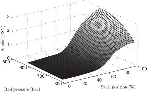
Smoke is measured in the unit of filter smoke number (FSN). The data consist of 1796 stationary grid measurements. Based on these data, a stationary LMN reference model with 22 LMs is generated, which is used for data generation and validation of the proposed online DoE procedure. In Figure 5, the smoke behaviour is exemplarily illustrated for a fixed EGR rate, timing of main injection and timing of pilot injection. Especially for variations in the swirl position, the smoke production shows a kink-like behaviour.

Figure 5. Illustration of an intersection plot of the smoke model. The output is depicted in the unit of filter smoke number (FSN) for a fixed exhaust gas recirculation (EGR) rate, timing of main injection and timing of pilot injection.

4.1.1. Online design of experiments

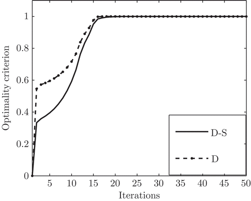
The initial DoE consists of 40 design points including all 32 corner points of the five-dimensional input space. The initial DoE is used to estimate the first LMN. Additionally, to the 40 initial design points, 203 iterative design points are generated according to the D-S-optimality criterion. In Figure 6, the D-optimality and the D-S-optimality criterion is exemplarily depicted for the optimization of a single design point. The comparison of both normalized criteria shows that a qualitatively similar improvement of the determinant of the Fisher information matrix is obtained. In order to obtain realistic data for the online training of the evolving LMN model, the output is obtained with the LMN reference model plus some additional smoke dependant noise.

Figure 6. Comparison of normalized optimality criteria. The D criterion denotes the determinant of the Fisher information matrix and the D-S criterion denotes the hybrid criterion combining the determinant of the Fisher information matrix with a distance measure.

4.1.2. Online training and model quality

Starting with the initial LMN, the model is incrementally evolved with each of the newly sampled data. For this purpose, the number of LMs is changed if the model complexity is not covered by the data.

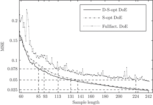
Here, a full quadratic structure is chosen for the regressor vector, which includes the linear, the quadratic as well as the mixed terms of all input channels. The principle of model validation is shown in Figure 7. A validation dataset is used to evaluate the quality of the evolving process model for each sample period by means of the means squared error (MSE). Here, 1000 space-optimal design points are chosen as validation data, in order to properly cover the whole input space. The proposed method for the generation of D-S-optimal designs is compared to a full factorial design and a purely S-optimal design of the same sample size, since these designs are commonly used in automotive applications. In this case, the full factorial design consists of three levels for each input channel. All possible combinations of these levels sum up to design points. The evaluation of the MSE was repeated 100 times for different initialization of all designs and the mean of the MSE is depicted in Figure 8. The D-S-optimal design achieves the fastest reduction of the model error. Since the full factorial design always consists of the same design points, although in a different order, the development of the mean of the MSE is not so smooth as for the S- and D-S-optimal designs. In Table 1, the number of design points are given which are needed to achieve an MSE of 0.078, 0.050 and 0.025, respectively. The application of the D-S-optimal design achieves a reduction of up to 10% of measurements compared to the space optimal design. The full factorial design needs a much higher number of measurements than the D- and D-S-optimal designs.

Table 1. Comparison of the number of design points for three particular model errors (MSE) and three experimental designs.

MSE	D-S-opt DoE	S-opt DoE	Full factorial DoE
0.078	85	93	113
0.050	131	141	224
0.025	227	242	x

Figure 7. Schematic illustration of the model validation.

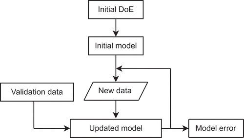
Figure 8. Illustration of the model quality in the form of the mean squared error (MSE) as a function of the sample size for the D-S-optimal design, the S-optimal design and the fullfactorial design.

4.2. Dynamic example

The generation of dynamic models becomes more and more important in the automotive sector for the calibration of the engine control unit. On the one hand, engine management systems are mainly based on stationary look-up tables, whereas driving cycles (e.g. New European Driving Cycle) for the assessment of the emission levels are dynamic. On the other hand, stationary measurements for the generation of stationary models are very time-consuming and, therefore, it is of great interest to derive stationary models from dynamic ones.

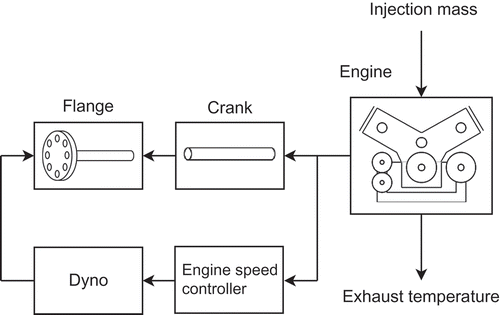
In this chapter, the generation of a dynamic exhaust temperature model is shown by means of the proposed online DoE procedure. For the generation of the data, a complex engine simulation software based on physical modelling is used [21,22]. In Figure 9, the engine model is depicted. The engine is excited by the injection mass and the output is the exhaust temperature. The sampling time is chosen to be 0.06 s. By a variable flange torque, the engine speed is controlled at 2200 rpm in order to guarantee well-defined operating conditions.

Figure 9. Engine with controlled engine speed.

4.2.1. Online design of experiments

For the identification of nonlinear dynamic system without prior knowledge about the underlying system, amplitude modulated pseudo random binary sequences (APRBS) are typically applied, cf. [9]. Therefore, an APRBS with a size of 300 samples is chosen as initial DoE. Based on the knowledge of previous work [23], a control horizon of is applied and after 700 sampling periods, the online procedure is stopped.

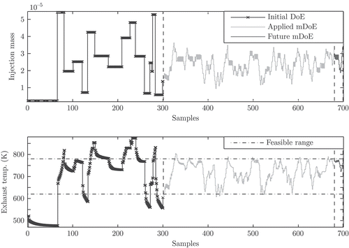
The compliance with output constraints is essential for the DoE in order to provide secure and stable operating conditions for the plant. Here, the feasible exhaust temperature ranges from 620K to 780K. The upper parts of the Figures 10–12 show snapshots of the DoE procedure and the lower parts show the associated system response with compliance of output constraints at different instants of time. In the upper part of Figure 10, the complete initial DoE sequence (line with crosses) is applied and the outlook on the future model-based DoE (mDoE) sequence consisting of 20 samples is given (solid black line). In Figure 11, a sequence of 190 mDoE samples (grey line) and in Figure 12, a sequence of 380 mDoE samples is applied. The associated exhaust temperature of the mDoE sequence stays well within the feasible range due to the model-based approach.

Figure 10. The upper part illustrates the design of experiments (DoE) given by the injection mass signal and the lower part indicates the associated system response (exhaust temperature). The snapshot is taken exactly when the initial DoE sequence (first 300 samples) is applied to the system. The outlook on the future model-based DoE (mDoE) ranges from the 301st to the 320th sample. For the future mDoE, the exhaust temperature is demanded to comply with the feasible range from 620K to 780K.

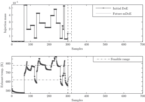
Figure 11. The upper part illustrates the design of experiments (DoE) given by the injection mass signal and the lower part indicates the associated system response (exhaust temperature). The snapshot of the DoE procedure has been taken after Figure 10 when 190 samples of the model-based DoE sequence (mDoE) have already been applied to the system. The applied mDoE sequence (301st to 490th sample, grey line) generates a system response that stays well within the feasible exhaust temperature range. The outlook on the future model-based DoE (solid black line) ranges from the 491st to the 510th sample.

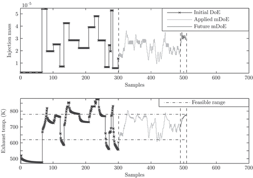
Figure 12. The upper part illustrates the design of experiments (DoE) given by the injection mass signal and the lower part indicates the associated system response (exhaust temperature). The snapshot of the DoE procedure has been taken after Figure 11 when 380 samples of the model-based DoE (mDoE) sequence have already been applied to the system (301st to the 680th sample, grey line). The applied mDoE sequence generates a system response that stays well within the feasible exhaust temperature range. The outlook on the future model-based DoE (solid black line) ranges from the 681st to the 700th sample.

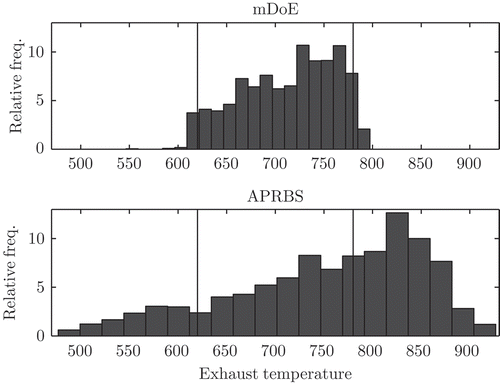
In Figure 13, the distribution of the exhaust temperature is evaluated for an optimal excitation signal under output constraints and for a reference APRBS with each having a sample size of 3000. The online model-based experiment design is capable of exciting the system in such a way that the output stays very well within the feasible exhaust temperature range. Slight limit violations are caused by the discrepancy between the predicted and the true exhaust temperature.

Figure 13. Distribution of the exhaust temperature for the model-based design of experiments (mDoE) and the amplitude modulated pseudo random binary sequence (APRBS). The optimal excitation signal is generated with a minimal and a maximal exhaust temperature of 620K to 780K.

4.2.2. Model quality

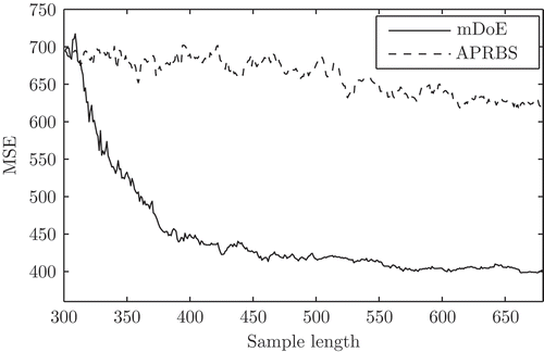
For the validation of the exhaust temperature model, the procedure of Figure 7 is used. The validation data consist of an APRBS and an optimal excitation signal, which is exemplary shown in Figure 14. The MSE is evaluated for 100 different training and validation data sets in order to obtain a statistically reliable result. In Figure 15, the development of the mean of MSE as as a function of the sample size is given. The optimized excitation signal achieves a much faster reduction of the mean of the MSE compared to the APRBS.

Figure 14. Exemplary illustration of the input and output validation data. The data consist of an amplitude modulated pseudo random binary sequence (APRBS) and of a model-based design of experiments (mDoE).

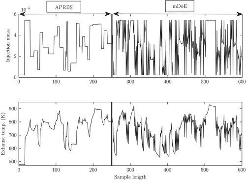
Figure 15. Development of the mean squared error (MSE) as a function of the sample length for the amplitude modulated pseudo random binary sequence (APRBS) and the model-based design of experiments (mDoE).

5. Conclusion

In the present paper, an online optimization procedure based on an evolving LMN for the generation of optimal excitation signals for nonlinear static and dynamic systems is proposed. The effectiveness of the proposed concept is demonstrated on two typical application examples of the automotive industry. In the first example, optimal excitation data for the estimation of a smoke model of a diesel engine is generated with the proposed D-S-optimality criterion. The example demonstrates that the proposed DoE procedure is capable of saving up to 10% of the training data compared to an S-optimal design when the same model quality is achieved. In the second example, the proposed online DoE method is applied to a nonlinear dynamic exhaust temperature model. The statistical assessment of the exhaust temperature models shows that optimal excitation signals improve the achievable quality significantly compared to APRB sequences. In addition, the presented online optimization method is capable of exciting the plant in such a way that input and output constraints are complied with.

The online DoE method proposed in this paper uses the Fisher information matrix as a basis for the required estimates of the parameter covariance matrix. As an effective alternative to the Fisher information matrix, methodologies which are based on the concept of the unscented Kalman filter (UKF) may be considered by the reader [24–27]. As opposed to the Fisher information matrix, UKF-based methods do not require the computation of the parameter sensitivities and can give accurate results for the covariance estimates of nonlinear systems. Further developments should, therefore, investigate the integration of UKF-based covariance matrix estimates for the proposed online optimization framework.

Acknowledgement

This work was supported by the Christian Doppler Research Association and AVL List GmbH.

References

- L. Ljung, System Identification: Theory for the User, 2nd ed., Prentice Hall Inc., Upper Saddle River, NJ, 1999.
- L. Pronzato, Optimal experimental design and some related control problems, Automatica. 44 (2008), pp. 303–325.
- G.C. Goodwin and R.L. Payne, Dynamic System Identification: Experiment Design and Data Analysis, Academic Press Inc., New York, 1977.
- M. Deflorian, F. Kloepper, and J. Rueckert, Online dynamic black box modelling and adaptive experiment design in combustion engine calibration, 6th IFAC Symposium Advances in Automotive Control 2010, Holiday Inn Munich, IFAC, Laxenburg, 12–14 July 2010, pp. 1–6.
- C. Hametner and S. Jakubek, Combustion engine modelling using an evolving local model network, Proceedings of the 2011 International Conference on Fuzzy Systems (FUZZ IEEE 2011), Taipei, 27–30 June 2011.
- S. Jakubek and C. Hametner, Identification of neurofuzzy models using GTLS parameter estimation, IEEE Trans. Syst. Man Cyber. B. 39 (2009), pp. 1121–1133.
- E. Lughofer, FLEXFIS: A robust incremental learning approach for evolving Takagi-Sugeno Fuzzy models, IEEE Trans. Fuzzy Syst. 16 (2008), pp. 1393–1410.
- C. Hametner and S. Jakubek, Engine model identification using local model networks in comparison with a multilayer perceptron network, Proceedings of the 2nd International Multi-Conference on Complexity, Informatics and Cybernetics: IMCIC 2011, Orlando, FL, 27–30 March 2011.
- O. Nelles, Nonlinear System Identification: From Classical Approaches to Neural Networks and Fuzzy Models, Springer, Berlin, 2001.
- E. Camacho and C. Bordons, Model Predictive Control, Springer, London, 2000.
- E. Walter and L. Pronzato, Identification of Parametric Models from Experimental Data, Springer, Berlin, 1997.
- G. Franceschini and S. Macchietto, Model-based design of experiments for parameter precision: State of the art, Chem. Eng. Sci. 63 (2008), pp. 4846–4872.
- T. Santner, B.J. Williams, and W. Notz, The Design and Analysis of Computer Experiments (Springer Series in Statistics), Springer, New York, 2003.
- S. Boyd and L. Vandenberghe, Convex Optimization, Cambridge University Press, New York, 2004.
- D. Luenberger and Y. Ye, Linear and Nonlinear Programming, Springer, New York, 2008.
- S. Richter, C. Jones, and M. Morari, Real-time input-constrained MPC using fast gradient methods, Decision and Control, 2009 held jointly with the 2009 28th Chinese Control Conference. CDC/CCC2009. Proceedings of the 48th IEEE Conference on, Shanghai, 15–18 December 2009.
- H.J. Ferreau, H.G. Bock, and M. Diehl, An online active set strategy to overcome the limitations of explicit MPC, Int. J. Robust Nonlinear Control. 18 (2008), pp. 816–830.
- Y. Wang and S. Boyd, Fast model predictive control using online optimization, IEEE Trans. Control Syst. Technol., 18 (2010), pp. 267–278.
- E.A. Yildirim and S.J. Wright, Warm-Start strategies in interior-point methods for linear programming, SIAM J. Optimiz. 12 (2002), pp. 782–810.
- C. Hametner, M. Stadlbauer, M. Deregnaucourt, S. Jakubek, and T. Winsel, Optimal experiment design based on local model networks and multilayer perceptron networks, Eng. Appl. Artif. Intel. 26 (2012), pp. 251–261.
- J.C. Wurzenberger, R. Heinzle, A. Schuemie, and T. Katrasnik, Crank-Angle resolved real-time engine simulation – integrated simulation tool chain from office to testbed, SAE 2009 World Congress (2009) Number 2009-01-0589 in Technical Paper Series, SAE International, Warrendale, PA.
- J.C. Wurzenberger, P. Bartsch, and T. Katrasnik, Crank-Angle resolved real-time capable engine and vehicle simulation – fuel consumption and driving performance, SAE 2010 World Congress (2010) Number 2010-01-0784 in Technical Paper Series, SAE International, Warrendale, PA.
- M. Stadlbauer, M. Deregnaucourt, C. Hametner, S. Jakubek, and T. Winsel, Online measuring method using an evolving model based test design for optimal process stimulation and modelling, Instrumentation and Measurement Technology Conference (I2MTC), 2012 IEEE International, Graz, IEEE, New York, 13–16 May 2012, pp. 1314–1319.
- R. Van Der Merwe, Sigma-point Kalman filters for probabilistic inference in dynamic state-space models, University of Stellenbosch, Stellenbosch, 2004.
- S.M. Baker, C.H. Poskar, and B.H. Junker, Unscented Kalman filter with parameter identifiability analysis for the estimation of multiple parameters in kinetic models, EURASIP J. Bioinforma. Syst. Biol. 2011 (2011), pp. 1–8.
- R. Schenkendorf, A. Kremling, and M. Mangold, Optimal experimental design with the sigma point method, IET Syst. Biol. 3 (2009), pp. 10–23.
- T. Heine, M. Kawohl, and R. King, Derivative-free optimal experimental design, Chem. Eng. Sci. 63 (2008), pp. 4873–4880.