A novel recursive subspace identification approach of closed-loop systems

Abstract

In this paper, a subspace model identification method under closed-loop experimental condition is presented which can be implemented to recursively identify and update the system model. The projected matrices play an important role in this identification scheme which can be obtained by the projection of the input and output data onto the space of exogenous inputs and recursively updated through sliding window technique. The propagator type method in array signal processing is then applied to calculate the subspace spanned by the column vectors of the extended observability matrix without singular value decomposition. The speed of convergence of the proposed method is mainly dependent on the number of block Hankel matrix rows and the initialization accuracy of the projected data matrices. The proposed method is feasible for the closed-loop system contaminated with coloured noises. Two numerical examples show the effectiveness of the proposed algorithm.

Keywords:

• subspace identification method
• recursive algorithm
• closed-loop system
• LQ decomposition

1. Introduction

Subspace Model Identification (SMI) has received much interest over the past two decades not only due to its convergency and numerical simplicity, but also for the state-space form that is convenient for estimation, filtering, prediction and control [1,2]. Most of these methods can achieve consistent estimates with open-loop or closed-loop data that construct input and output block Hankel matrices in order to retrieve certain subspaces related to the system matrices [3–7]. However, these algorithms, which are only appropriate for offline identification, are difficult to implement online due to huge computational load of singular value decomposition (SVD) of related matrices.

As far as we know, in many cases, it is necessary to have a model of the system available online while the system is in operation [8], such as the design of an adaptive model predictive controller. A possibility is provided by identifying a system under closed-loop condition using a recursive updating of the model. It meets the requirement that one of the dimensions of the block Hankel matrices involved needs to go to infinity in offline identification since updating technique is used. The main problem with the implementation of recursive SMI algorithms under closed-loop condition is to find alternative ways for SVD or avoid the application of the SVD. Several recursive algorithms for closed-loop subspace identification have been developed. In order to obtain unbiased parameter estimates, the vector auto regressive with exogenous input models from the work of [9] has been introduced and the Projection Approximation Subspace Tracking (PAST) algorithm method is used to update the signal subspace in [10]. The problem of recursive closed-loop subspace identification in [11] is presented by two linear optimization problems and subspace tracking techniques are developed to recursive SMI based on the relationship between sensor array processing (SAP) and SMI problems. In this paper, we present a new recursive subspace identification method under closed-loop conditions based on the orthogonal decomposition, which has been inspired and motivated by the offline version of the ORT-based method [6]. The contributions of this paper are twofold. First, the approach overcomes the main difficulty in the identification of closed-loop system due to correlation between external inputs and noises resulting in biased estimates of plant model parameters. It provides asymptotically unbiased estimates of system matrices as the number of data samples goes to infinity. Second, this recursive approach overcomes practical difficulties of most closed-loop methods characterized batchwise identification with huge number of input and output sequences, such as acquiring, storing and analysing large data sets. We present a new updating scheme for the projected data matrix which applies sliding window technique to update data sequences to infinity and develops recursive construction for the LQ decomposition. Based on the propagator type method in the array signal processing, we obtain the subspace spanned by the column vectors of the extended observability matrix without SVD. In the simulation, the proposed method can achieve unbiased estimates in the presence of coloured noises in closed-loop system.

The remainder of this paper is organized as follows. In Section 2, we state problem formulation and introduce state-space model and notation. In Section 3, the projected data matrix is constructed online by the updating technique. In Section 4, a recursive identification algorithm is emphasized. In Section 5, two numerical examples are given and the results show the effectiveness of the proposed algorithm. Finally, in Section 6, we present the conclusion and prospect of the future research.

2. Problem formulation

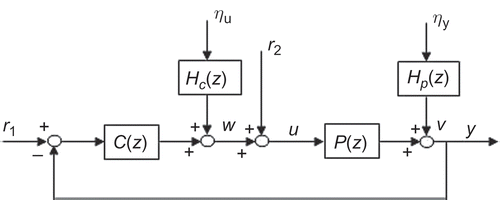
Consider a closed-loop system depicted in Figure 1. The plant is assumed to be modelled by , represented as a finite dimensional state-space model in the following. Let us assume that the signals and are observed. The disturbance signals and are white noise with mean zero. The matrices and are related noise filters, respectively. Furthermore, it is assumed that

Figure 1. Block schematic representation of the closed-loop configuration.

A1:	=	The feedback system is wellposed in the sense that are determined uniquely if all the external signals are given;
A2:	=	The controller is known and stabilizes the closed-loop system;
A3:	=	The exogenous inputs satisfy persistent exciting (PE) conditions and are uncorrelated with the white noises and ;
A4:	=	The exogenous inputs and noises are second-order jointly stationary processes with mean zero;
A5:	=	There is no feedback from to .

Based on the configuration of Figure 1, we state the following closed-loop identification problem. Given the exogenous inputs and input output u, y, we derive a subspace identification method to estimate state-space models of the plant recursively that is independent of the noise properties.

2.1. State-space model

Define and . The whole infinite history of stationary processes is given. The Hilbert spaces are generated by second-order random variables of the exogenous inputs and joint input–output signals which are denoted by and . Then the ambient Hilbert space is given by , where ‘’ denotes the closed vector sum. We obtain the orthogonal projection of w onto

(1)

where denotes the orthogonal projection onto and is called the deterministic component of w. It follows that

(2)

where is the orthogonal complement and is called the stochastic component of w. Under the assumption that exogenous inputs are feedback-free, the joint input–output process w has the orthogonal decomposition

(3)

or

(4)

Moreover, and are mutually uncorrelated,

The further details of orthogonal decomposition of joint input–output process can be referred in [6].

The plant of the closed-loop system shown in Figure 1 can be expressed with transfer function as

(5)

The orthogonal projection of Equation (5) onto is obtained based on the above the decomposition results,

(6)

Due to the external input signal, r is uncorrelated with the noise , all elements of are close to 0 as . Then we rewrite Equation (6) as

(7)

where and . So the estimate of plant can be obtained from the deterministic component . The plant is expressed into a deterministic state-space form as:

(8)

where the system matrices , , and .

Define the finite history of second-order random variables of exogenous inputs which is a subspace of at the time period . Then, we take the orthogonal projection of Equation (6) onto the space and obtain,

(9)

where and . Based on the property of orthogonal projection, see Appendix A, we can obtain the following relationships due to with dim,

(10)

2.2. Notation

Given the current data sequences , we construct reference input block Hankel matrix as:

(11)

where the number of block rows i is a user-defined index and the number of columns is , which implies that all given data samples are used. In general, we can choose this index i with experience or based on the results of many experiments. In a similar way, we construct block Hankel matrices and and also define

(12)

where the subscripts p and f denote the past and the future, respectively. The extended observability matrix is defined as:

(13)

The lower block triangular Toeplitz matrix is defined as:

(14)

3. Recursive update of the projected data matrix

In this and the next sections, we consider the projected data to recursively identify system matrices of the plant . The first step of the recursive algorithm is to construct and update the projected data matrix.

3.1. Construction of the projected data matrix

Based on the orthogonal projection in previous section, we define the projected data matrices and and the stacked matrix .

Lemma 3.1: Given block Hankel matrices , and with data sequence , the projected data matrix can be obtained via the LQ decomposition as follows,

(15)

where , and . Then the projected matrix is obtained by

(16)

where , and .

Proof: In the general case, the matrices A and B can be expressed as linear combinations of orthogonal matrix in terms of LQ decomposition as:

Thus, the orthogonal projection of the row space of A on the row space of B is denoted by

Applying the above result, we compute the orthogonal projection of the row space of onto and mark the dimension of each matrix below and then have

In a similar way, we also obtain

It should be noted that rank() must hold in order to apply the LQ decomposition in the next step. To ensure this condition, we have assumed that has PE condition of order . Then, the component has PE condition of order [12].

3.2. Update the projected data matrix by sliding window

At the current time instant t, the data sequence is given. We define

(17)

and each element is , where , and . According to Lemma 3.1, we have the LQ decomposition and the corresponding projected data matrix is

(18)

At the th time instant, new observed data is obtained to construct data vectors as following:

(19)

In a similar way, we obtain new data vectors and . Thus,

(20)

Then, the new column is added and the old column is eliminated and a new data matrix is obtained as . The data matrix is expressed into the LQ decomposition form:

(21)

where and are unknown. We introduce an intermediate matrix

(22)

Define and , is the ith row of the matrix ,

(23)

and is the ith row of the matrix ,

(24)

Clearly, the elements of the row are known but those of are mostly unknown. Based on the definition of the LQ decomposition, the intermediate matrix satisfies,

(25)

and

(26)

Due to the orthogonality of matrices and , it is easy to obtain

(27)

Unfold Equation (27), the corresponding elements of both sides are equal and each element of the updated matrix can be computed via the Algorithm I in Table 1. In a similar way, we can obtain the matrix .

Table 1. Algorithm I: update of the projected data matrix.

Initial , ,
For do
For do
End for
End for

Note that we can obtain better estimates of initial projected data matrices and from batchwise identification in order to avoid suffering from the convergence problem.

4. Recursive subspace identification of closed-loop system

After recursively updating the projected data matrix at th time instant, we can obtain

(28)

Then adjust the projected data matrix and compute the LQ decomposition as follows:

(29)

where , and . Since is orthogonal, it is enough to take the LQ decomposition of [13]. Clearly the second LQ decomposition can be performed in a computationally less expensive manner. The future output has the following expression directly from Equations (8) and (29):

(30)

where the state sequence is . Using to post-multiply Equation (30), we obtain

(31)

4.1. Recursive estimation of a basis of Γⁱ_d

Consider the noise-free case, since the extended observability matrix with , the matrix has, at least, linearly independent rows to guarantee the full rank, the following partition of the observation vector can be introduced:

(32)

where and are the components, respectively, to the rows and rows of . Thus, there exists a unique operator , such as

(33)

Moreover, an estimate of the extended observability matrix is available by estimating and that is . In order to develop a recursive minimization algorithm, we introduce the forgetting factor and obtain the cost function with a finite exponentially weighted sum as:

(34)

The minimization of such a criterion is recursively feasible by applying a classic recursive least squares approach. The estimation algorithm is summarized as Algorithm II in Table 2.

Table 2. Algorithm II: estimate of the extended observability matrix.

Initial , and
For do
End for

4.2. Computing the system matrices

By using the shift-invariance property of the extended observability matrix , the estimates and are directly obtained in the non-recursive case:

(35)

Once the matrices and are fixed, the estimates of and can be computed. Pre-multiplying Equation (30) by and post-multiplying by yield,

(36)

Given the estimate of the extended observability matrix , the term is linear with respect to parameters, so that we can easily obtain and by the least squares method.

5. Numerical examples

5.1. Example 1

In order to illustrate the performance of the proposed method in this paper, we consider the closed-loop system depicted in Figure 1. There are three cases of the controller and the plant displayed in Table 3. The noise models are given by

Table 3. Transfer functions used for simulation.

	Controller	Plant
Case 1
Case 2
Case 3

The reference inputs and are zero mean Gaussian white signals with variances . The noise input is uncorrelated with the reference signals r and also is zero mean Gaussian white signal with variance . For the data Hankel matrices, the user-defined index is chosen . We use former 20 data samples to calculate the estimates of initial matrices. The order of the plant is assumed to be known as .

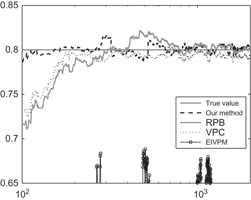
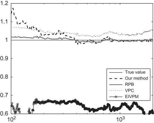
We compare the representative recursive subspace algorithms VPC [10], RPB [11] and EIVPM [14] with our method. Trajectories of estimated poles of the plant in three cases averaged over 30 independent Monte Carlo Simulation (MCS) and are displayed in Figures 2–4. As expected from Figures 2 and 3, the open-loop method EIVPM gives a biased result both in case 1 and case 2 because of the correlation of future inputs and past noises under the closed-loop condition. For case 1 and case 2, Figures 2 and 3 demonstrate that VPC, RPB and our method have a remarkable ability to track the poles. As the number of samples increases, the results of estimated poles can be consistent with true value. It is also observed from Figures 2 and 3 that the variance around the mean trajectories is much larger for the VPC than for our method and RPB.

Figure 2. Trajectories of estimated pole of the plant in case 1 by RPB, VPC, EIVPM and our method.

Figure 3. Trajectories of estimated pole of the plant in case 2 by RPB, VPC, EIVPM and our method.

Figure 4. Trajectories of estimated pole of the plant in case 3 and in case 3 with no noise by RPB and our method.

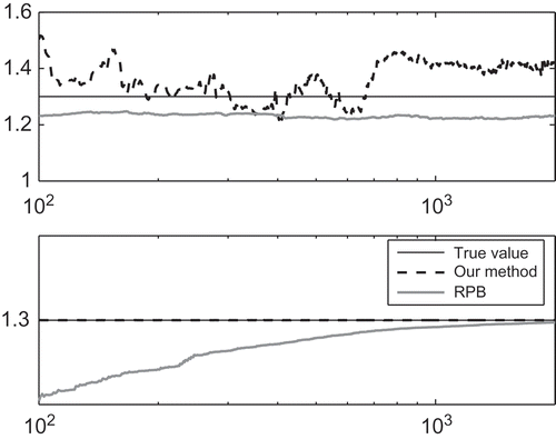
For case 3, there seem to be some difficulties in obtaining unbiased estimates of the plant by RPB and our method, as shown in the upper subplot of Figure 4. We note that the plant is an unstable system of which the pole is outside the unit circle. This observation does not mean that our method cannot always be applied to unstable systems. If the noise variance is reduced to zero, the identification result of the unstable plant can follow the estimated pole trajectory much better in the bottom subplot of Figure 4. Moreover, our method presents faster convergence than the RPB method.

5.2. Example 2

We consider the following fourth-order multi-variable system described by

where

The innovation is an independent white noise sequence. The signal to noise ratio (SNR) is tuned to 20 dB.

To create a closed-loop system, the feedback gain matrix is chosen as that stabilizes the above system under closed loop over the whole trajectory. The reference signals and are zero mean Gaussian white noise signals with variance . We assume that the dimension of the plant is .

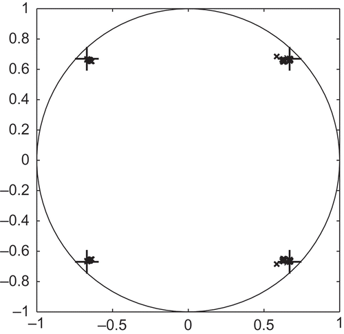
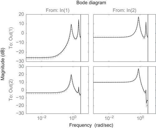
We performed 100 MCS experiments with different initial values which are properly chosen as zero or unit matrices. In Figure 5, poles of the true system are marked by ‘+’. The poles of the identified system are shown by ‘x’ or shaded region which are estimated by the proposed method in the paper. It can be seen that our method successfully captures poles of the true system. Moreover, the red lines show the bode plots of the true system in Figure 6. Bode plots of the estimated system in 100 MCS experiments by our method are displayed in dotted lines. It is observed from the Figure 6 that the true bode plots are covered by the estimated curves. We conclude that our method gives unbiased estimates of the identified system, though the fluctuation of the estimates of the output 1 from input 1 in lower frequency is somewhat large.

Figure 5. Poles of the identified system in closed-loop by the proposed method.

Figure 6. Bode plots of the identified system in closed-loop by the proposed method.

6. Conclusion and future work

Under the assumption that the order of a plant system to be identified is a priori known, we derive a recursive closed-loop SMI algorithm. The proposed algorithm updates the projected data matrix through linear equations and estimates the extended observability matrix based on the propagator method. The effectiveness of the algorithm has been demonstrated by two numerical simulation examples.

However, it should be noted that since the projection is onto the finite data space , the projected data are not purely deterministic and do contain some residuals, or noises. It is clear as the window size that is

and then we would recover the perfect noise-free input signals.

The future work is to explore and improve the issues in terms of accuracy and speed of convergence of the algorithm.

Appendix A. The property of orthogonal projection

Let X, and be three spaces with , so that dim. Find and denote

then

so that we have

In addition, a similar property holds for conditional expectation, if we consider are (sub)-algebras, can be replaced by E.

References

- S.J. Qin, An overview of subspace identification, Comput. Chem. Eng. 30 (10–12) (2006), pp. 1502–1513.
- P. Van Overschee and B. De Moor, Subspace Identification for Linear Systems: Theory, Implementation, Applications. Dordrecht, Kluwer Academic Publishers, 1996.
- M. Gilson and G. Mercère. Subspace-based optimal IV method for closed-loop system identification, in Proceedings of the 14th IFAC Symposium on System Identification, IFAC, Newcastle, 29–31 March 2006, pp. 1068–1073.
- P. Van Overschee. Closed loop subspace system identification, in Proceedings of the 36th IEEE Conference on Decision and Control, IEEE, San Diego, CA, 10–12 December 1997, pp. 1848–1853.
- A. Chiuso and G. Picci, Consistency analysis of some closed-loop subspace identification methods, Automatica 41 (3) (2005), pp. 377–391.
- T. Katayama, H. Kawauchi, and G. Picci, Subspace identification of closed-loop system by the orthogonal decomposition method, Automatica 41 (5) (2005), pp. 863–872.
- G. Mercère, L. Bako, and S. Lecoeuche, Propagator-based methods for recursive subspace model identification, Signal Process. 88 (3) (2008), pp. 468–491.
- L. Ljung, System Identification: Theory for the User, Prentice-Hall, Upper Saddle River, NJ, 2002.
- T. Gustafsson, Instrumental variable subspace tracking using projection approximation. IEEE Trans. Signal Process. 46 (3) (1998), pp. 669–681.
- P. Wu, C. Yang, and Z. Song, Recursive subspace model identification based on vector autoregressive modelling, in Proceedings of the 17th IFAC Symposium on Automatic Control, IFAC, Seoul, 6–11 July 2008, pp. 8872–8877.
- I. Houtzager, J. Van Wingerden, and M. Verhaegen, Fast-array recursive closed-loop subspace model identification, in Proceedings of the 15th IFAC Symposium on System Identification, IFAC, Saint-Malo, 6–8 July 2009, pp. 96–101.
- I. Markovsky, J.C. Willems, P. Rapisarda, and B. De Moor, Algorithm for deterministic balanced subspace identification, Automatica 41 (5) (2005), pp. 755–766.
- T. Katayama and H. Tanaka, An approach to closed-loop subspace identification by orthogonal de-composition, Automatica 43 (2007), pp. 1623–1630.
- G. Mercè re, S. Lecoeuche, and C. Vasseur, A new recursive method for subspace identification of noisy systems: EIVPM, in Proceedings of the 13th IFAC Symposium on System Identification, Elsevier, Rotterdam, 27–29 August 2003, pp. 1637–1642.