Modelling neuromuscular blockade: a stochastic approach based on clinical data

Abstract

During surgical interventions, a muscle relaxant drug is frequently administered with the objective of inducing muscle paralysis. Clinical environment and patient safety issues lead to a huge variety of situations that must be taken into account requiring intensive simulation studies. Hence, population models are crucial for research and development in this field.

This work develops a stochastic population model for the neuromuscular blockade (NMB) (muscle paralysis) level induced by atracurium based on a deterministic individual model already proposed in the literature. To achieve this goal, a joint Lognormal distribution is considered for the patient-dependent parameters. This study is based on clinical data collected during general anaesthesia. The procedure developed enables to construct a reliable reference bank of parametrized models that not only reproduces the overall features of the NMB, but also the inter-individual variability characteristic of physiological signals. It turns out that this bank constitutes a fundamental tool to support research on identification and control algorithms and is suitable to be integrated in clinical decision support systems.

Keywords:

• stochastic modelling
• neuromuscular blockade level
• simulation
• validation

1. Introduction

Dynamic mathematical modelling in physiology and medicine has a long history and presents many scientific and technical challenges. In fact, human physiology exhibits a multitude of features of complexity [1] as well as a large inter-individual variability that must be accounted for when trying to provide appropriate representations of physiological and medical systems. Mathematical modelling is becoming increasingly important in physiological and clinical research. For instance, mathematical models can be used heuristically to test alternative scientific hypotheses, and assist in experimental design, carrying out trials through computer simulation in order to identify what is likely to be the most appropriate experimental configuration [1].

Physiological and medical systems have been modelled from both data-driven and process-driven approaches. The former seeks mathematical expressions that adequately fit experimental data. The latter has been possible with the increase of the knowledge of the underlying physics and chemistry of physiological mechanisms (including physicochemical dynamics, transport and storage mechanisms, and multiple types and level of control action). These models are typically deterministic in the sense that the time evolution is entirely pre-determined by an exact knowledge of the initial conditions and the model parameters. These are estimated from data available for model identification and, henceforth, considered as accurately known. Thus, the population is represented by a single set of parameters representing the average individual. It is, however, acknowledged that this established procedure produces models that fail to represent the large biological variability observed in physiological and clinical data.

The present work proposes a modelling procedure that allows the replication of the inter-individual variability observed in physiological data and also improves on existing models for modelling adequately each individual.

To achieve these goals, a general approach based on representing the population characteristics is devised in the context of the application to neuromuscular blockade (NMB) induced by atracurium. Thus, a population model for NMB based on an existing minimally parameterized parsimonious (MPP) model is developed. Furthermore, modelling of individual NMB is achieved based on the population model and the minimization of a suitable loss function. It is worth noting that the availability of adequate population models is desirable in many scientific areas, and in particular in biomedicine, since they allow the experimentation through computer simulation in situations where experimentation is limited, in particular, for ethical reasons. For instance, in the case study of NMB induced by atracurium considered here, the population model allows the design of a procedure to calculate the required atracurium individualized dosage to attain a pre-specified NMB level [2].

The paper is organized as follows. The remaining of this section reviews the literature concerning models for NMB and describes the clinical data set available for this study. In Section 2, a stochastic population model for the NMB is developed and its output is validated in Section 3. Section 4 describes individual modelling of NMB and finally Section 5 draws conclusions.

1.1. Models for NMB

Muscle relaxant drugs are frequently given during surgical operations. The non-depolarizing types of relaxant act by blocking the neuromuscular transmission, thereby producing muscle paralysis (relaxation). The physiological effect induced by drug administration is described by deterministic pharmacokinetic and pharmacodynamic (PKPD) models that represent the interaction of the drug with the patient’s body. Since PKPD model parameters have physiological meaning and allow for parameter interpretation, several approaches to obtain a PKPD model are found in the literature. These approaches consist mainly on choosing a PK compartmental model for the quality of the fit, its simplicity or some clinical reason [3], extending existent PKPD models or including a link model to improve the quality of the model [4,5,9].

It is, however, acknowledged that parameters of pharmacokinetic models are difficult to estimate simultaneously since these models predict a pattern of concentration over time that is close to a mixture of declining exponential functions, with the amplitudes and decay times of the different components corresponding to functions of the model parameters [6]. These non-identifiability problems led to other approaches in which the models are built for a specific purpose, such as a controller design, or purely from a data-based approach with parameters that are meaningless from the physiological point of view [7].

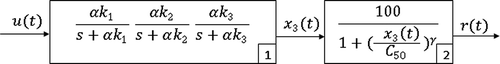
Alternative models to PKPD models are the reduced complexity models that have the advantage of avoiding identifiability problems while retaining some compartmental interpretation. In particular, [8] proposed the MPP model for the NMB induced by the muscle relaxant atracurium. This model has a linear part represented by the first block in Figure 1 and a non-linear part which is a static Hill equation, represented in block 2 in Figure 1.

Figure 1. Block diagram of the NMB model for atracurium, the MPP model.

The linear part of the MPP model may be represented by the following system of differential equations,

(1)

where the dot denotes the time derivative, are the state variables, , , are the known process parameters [8], and is an unknown patient-dependent parameter. Thus, the linear part of the model relates the input of the system, i.e. drug infusion rate or atracurium dosage to the state variable The Hill equation in block 2,

(2)

relates the state variable to the output of the model, the blockade level, . The parameter is a known process parameter [8], and is a patient-dependent parameter. This MPP model does not present identifiability problems while allowing the study of other variables of interest such as the individual maintenance dose necessary for its effect (NMB level) to attain a target profile.

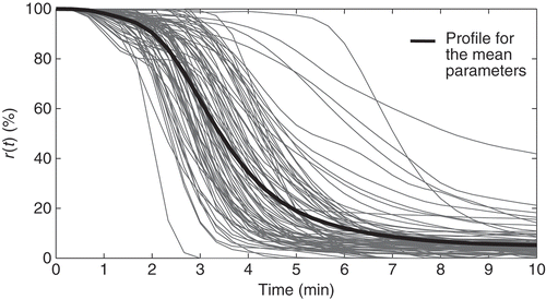
The dynamic evolution of the NMB described by Equations (1) and (2) is deterministic. As with other deterministic models for the NMB, this model fails to represent the biological diversity and variability present in the experimental data. This issue is illustrated in Figure 2: the NMB for the muscle relaxant atracurium of 84 patients undergoing general surgery is represented by (_) and the output of the MPP model with parameters set to the mean values obtained from clinical data is represented by (⁃).

Figure 2. NMB level of 84 patients undergoing general surgery (_) and NMB for mean parameters (⁃).

1.2. Clinical data set

For this study, a database of 84 patients undergoing general surgery (43 males, 38 females and 3 unknown gender) is available. The patients characteristics regarding age and weight are summarized in Table A1. The level of muscle relaxation is measured from an evoked electromyography (EMG) obtained from the patient’s hand by electrical stimulation of the adductor policies muscle to supramaximal train-of-four stimulation of the ulnar nerve [9]. The variable is normalized between 0%, full paralysis and 100%, full muscular activity and is sampled every 20 seconds. For clinical reasons, a bolus of atracurium of is always administered at the beginning of a surgery with the purpose of inducing a rapid decrease in the NMB level. The NMB () for the 84 patients is represented in Figure 2. After 10 minutes, the administration of atracurium is controlled by an automatic system with a fixed set-point of 10%. Table A2 summarizes the data concerned with the clinical procedure: duration of the surgery, the mean rate of atracurium administered after 75 minutes, denoted by the steady-state dose the mean blockade level after 75 minutes, , i.e. the blockade level in steady state. Note that the coefficient of variation for in the steady state is small (less than 10%) since the data are obtained from an automatic control system tuned to attain a steady-state reference.

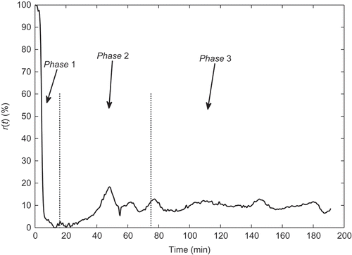
Finally, it is important to take into account the standard anaesthetic procedure and the NMB response which lead to division of the NMB response into three distinct phases as illustrated in Figure 3: the induction phase (phase 1), corresponding to the elapsed time between the initial bolus administration and the instant when the patient begins his recovery, usually with duration greater than 10 minutes; the transient phase (phase 2) which is the time interval between and 75 minutes after the initial bolus administration; and finally, the steady-state phase (phase 3) which begins at the 75th minute and finishes with the end of the clinical procedure, T.

Figure 3. Observed signal and its phases.

2. A population model

The aim is to construct a population model able to reproduce not only the overall characteristics of the physiological response but also the inter-individual variability. The first step is to consider a model describing the relationship between the drug dosage and its physiological effect in terms of one or more parameters for each individual. Justifiably, in this work, in the context of NMB, the choice belongs to the MPP model described in Section 1.1 which depends on two parameters, and The second step is to describe the distribution of the parameters in the population, meaning that in the present case study, the parameters () are considered random variables whose joint distribution must be specified. Hence, all the state variables in Equations (1) and (2) are random variables too and the system is rewritten as a stochastic system as follows.

(3)

with () a random vector with joint density function .

There are two possible approaches for the specification of the joint density function The first is to consider the empirical distribution function. This approach has the clear disadvantage of not allowing the generation of values outside the range of observed values. The second approach is to consider a probabilistic model. Since the Lognormal distribution is frequently associated with physiological parameters [10,11] and with positive quantities [12], it seems reasonable to entertain a bivariate Lognormal distribution as a possible joint probability distribution for (). This means that has a Bivariate Normal distribution, , with mean and covariance matrix,

where and are the parameters of the distribution.

The joint probability density function of () is defined as

(4)

with , and The superscript T indicates the transpose and is the determinant of the matrix .

To fully specify the joint probability distribution of the parameters of this distribution, and , are estimated from a sample of values obtained from the clinical data available for model identification and described in Section 1.2.

2.1. Construction of the sample

A sample of values of is constructed by fitting the MPP model described by Equations (1) and (2), to the observed NMB level, in the database. Here, the fitting procedure will be achieved in two steps. In the first step, estimates for are obtained using the algorithm proposed by [13] based on the minimization of the mean squared error. In the second step, these estimates are optimized so that the fit is improved.

There are two key issues in this optimization procedure. The first issue concerns the sensitivity of the model to the parameters In fact, it is acknowledged that models are sensitive to input parameters so that small changes in the input values result in significant changes in the output. Thus, a sensitivity analysis to determine the response of the MPP model, Equations (1) and (2), to changes in the parameters is carried out as follows. A factorial design set-up is adopted with each parameter taking the values with obtained in step 1 of the estimation procedure. The model is run for all the 25 possible combinations, with the atracurium dosage regimen of an initial 500 bolus followed by a continuous infusion rate of 8.0 (estimated as the sample mean value for the 84 patients) after 10 minutes.

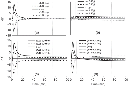
The plots in Figure 4 summarize the results. The plots represent the mean differences between the reference curve generated at and at the other parameter combinations. The results indicate that the major effect of parameter is in phase 1 and an increase in will decrease in phase 1 and phase 2; the major effect of parameter is in phase 3 and an increase in will decrease in phase 2 and phase 3.

Figure 4. Mean difference between the reference curve generated from MPP Model with the estimated parameters and and the curves obtained by varying: (a) only ; (b) only ; (c) and in the same amounts and same direction (increase or decrease both) and (d) and in the same amounts but opposite direction: increase () decrease (), for the 84 cases. Vertical dashed lines limit the three phases.

The second issue concerns the definition of an appropriate metric to assess the goodness of the fit. Such a metric measures the distance between the observed relaxation level, , and the fitted value, obtained from the MPP model and must be defined taking into account the standard anaesthetic procedure and resulting the NMB response, as described in Section 1.2 and Figure 3. Thus, a global measure of the distance between and is replaced by a phase-dependent measure defined as

(5)

where

Now, having defined an appropriate measure, a particular fit is considered acceptable if the following criterion is met:

(6)

These thresholds are justified by the parameter sensitivity analysis described before. In fact, when changes of 15% in the parameters are performed, i.e. take the values , , and , the following mean values for and are obtained: , and Considering that recovery phase is not included in the sensitivity analysis but some of the clinical cases are already recovering in phase 3, the thresholds maybe interpreted as allowing for a 15% variation in the estimated parameters ascribable to measurement errors.

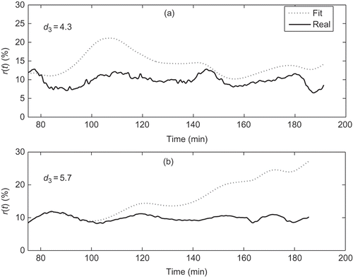
Figures 5–7 illustrate the adequacy of criterion 6. Figure 5 represents phase 1 of with a good fit in (a) corresponding to , an acceptable fit in (b) with and an unacceptable fit in (c) with . Figure 6 represents four different fits of phase 2. Cases (a) and (b) with and , respectively, have acceptable fits but cases (c) and (d), with and , respectively, present deviations that are not acceptable. Finally, in Figure 7, fits for phase 3 are represented. Case (a) with is considered acceptable but case (b) with is clearly unacceptable.

Figure 5. Phase 1. Cases (a) and (b) are acceptable but the case (c) is not acceptable.

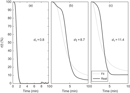
Figure 6. Phase 2. Cases (a) and (b) are acceptable but the cases (c) and (d) are not acceptable.

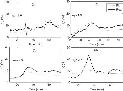
Figure 7. Phase 3. The case (a) is acceptable based on the phase criterion but the case (b) is not.

The above study suggests that varying the parameters and estimated in step 1 of the procedure may lead to an improved fit in (some of) the cases. Accordingly, each one of the initial 84 pairs of estimated parameters is varied in the range . The final estimate corresponds to the pair that simultaneously satisfies criterion (6) and minimizes the weighted criterion This optimization procedure leads to a database of 48 cases, hereafter denoted .

Thus, a sample of 48 pairs of values , is obtained. This sample is used next to check the hypothesis of bivariate normality of and estimate the parameters of the distribution (4).

2.2. Specification of the joint distribution for (α, γ)

To check the assumption of bivariate normality of (, ), graphical plots and formal hypothesis tests are used [14]. The BiNormal distribution, BN, is a special case of the multivariate normal distribution that lends itself to a geometrical representation and interpretation in a scatter plot. In particular, if and are independent random variables, their joint BN distribution is given by

(7)

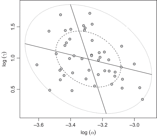
It is then easy to see that, in polar coordinates, each circle centred in the origin is the region of the plane that contains P% of the values. In the more general case, where the two variables are not independent, the corresponding regions of the plane are ellipses [15]. Figure 8 represents the bivariate boxplot of The inner ellipse is called the hinge and contains 50% of the data. The fact that no observations lie outside the fence which is the outer ellipse and contains 99% percent of the data, indicates the absence of possible troublesome outliers [16–18].

Figure 8. Bivariate boxplot for .

To test for the null hypothesis of multivariate normality, several tests are performed, namely: tests based on skewness and kurtosis [19,20] of the data and tests based on distance measures. Among the group of tests relying on distance measures, the following are considered: the generalized Shapiro–Wilk test [21,22] and the Shapiro–Francia test [23–27]. Moreover, the E-statistic (Energy) [28,25] test based on Euclidean distance and a test based on Mahalanobis distance and implemented in the package QRMlib in R [29,30], are also applied. The p-values for the above-mentioned tests reported in Table 1 do not allow the rejection of bivariate Lognormal joint distribution for and at the usual 5% level of significance.

Table 1. Tests for multivariate normality using the group of tests.

Test	p-Value
Skewness	0.893
Kurtosis	0.492
Generalized Shapiro–Wilk	0.390
Shapiro–Francia	0.250
E-statistic (Energy)	0.389
Based on Mahalanobis distances	0.809

The parameters μ, Σ of the BN(μ, Σ) distribution (4) are estimated by the method of moments from the database yielding asymptotically unbiased and consistent estimates.

Henceforth, the joint distribution for the parameters is the following:

(8)

with and

3. Validation of the model

In this section, the model given by Equations (3) and (8), hereafter designated by SMPP, is validated as a population model. This means determining whether the model represents adequately the inter-individual variability observed as well as the overall features of the NMB. To do so, the Monte Carlo method is especially appropriate since it allows to obtain an (almost) unlimited number of outputs, the NMB response in this case, by generating an input matrix of values through random sampling from the Lognormal distribution (8).

Thus, a bank of 500 pairs of parameters is randomly generated from Equation (8) and the corresponding response, to a single bolus administration is calculated, =. To assess further the validity of the proposed model as a population model, the data set [31], proposed by [9] is also included in this study.

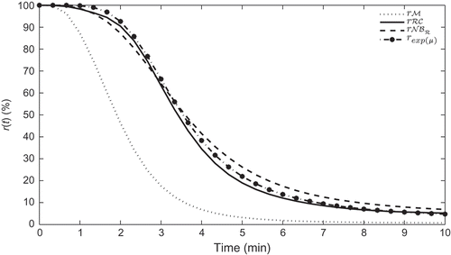
Figure 9 represents the mean response profiles for the three data sets. Clearly, the profiles for and are the closest. The distance given by Equation (5) between the profiles are and

Figure 9. Mean response profiles for the data , , and the response profile for the mean parameters, .

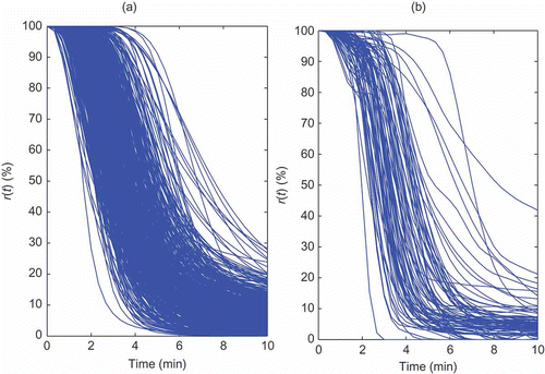
Figure 10 represents = in (a) and in (b). Note that, the comparison between the behaviour of collected data and the generated data must be restricted to the first 10 minutes since only in this interval of time, do both data sets represent the answer of the system to the same input (initial bolus administration). Also, note that, after the initial 10 minutes, the data collected in the surgery room, resulting from automatic control delivery system, may present non-zero infusion dose. It seems clear from Figure 10 that with the proposed population model, the inter-individual variability observed in NMB is achieved. To enforce this observation, the comparison between and is further carried out using statistical techniques.

Figure 10. The first 10 minutes of the NMB for 500 simulated cases, (a), and for the 84 real cases, (b).

Table 2 summarizes a set of statistics characterizing the NMB for the two data sets, at three different time points. Taking into account that the NMB level ranges from 0% to 100% and that there is some noise level present in clinical NMB records, the values of the statistical measures for the two data sets may be considered to be very close.

Table 2. Summary statistics of NMB for the clinical data set and the simulated data set for three different time points.

Time	Data set	Min.	Max.		S	CV (%)
t = 1 min		90	103	98	2.1	2.2
		79	100	99	2.9	2.9
t = 3 min		0.0	99	63	24	38
		7.2	100	64	21	32
t = 9 min		0.0	46	5.7	6.7	118
		0.1	35	8.0	5.9	75

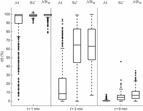
Next, observation times minutes are chosen as representatives of the 10 minutes and boxplots for the NMB response at these times for the three data sets are constructed and represented in Figure 11. Clearly, the distribution of the NMB obtained from the proposed stochastic model, is closest to that of the patient database,

Figure 11. Boxplot for the in three different instants, t = 1, 3, 9 min and for the three data.

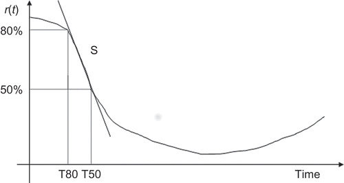
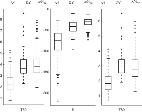
An additional validation is performed by means of the shape parameters, namely T80, T50 and S represented in Figure 12 and used to characterize the patient response to the initial bolus dose [9,32,33]. T80 is the elapsed time between the bolus administration and the time the response becomes less than 80%, T50 is the elapsed time between the bolus administration and the time the response becomes less than 50% and S is a slope parameter. These shape parameters are computed for the profiles in Figure 9 for the three data sets.

Figure 12. Shape parameters used to characterize induced by an initial bolus administration.

The values of the shape parameters for the profiles given in Table 3 as well as the computed difference to the indicate that the profile of is closer, in this sense, to . Note that the differences are all positive emphasizing the bias of the profile. The shape parameters are also computed for the three data sets and the corresponding boxplots represented in Figure 13 indicate good agreement between data sets and

Table 3. Shape parameters for the three profiles and differences for .

	Shape parameters
Data set	T50	S	T80
	3.750	−31.68	2.803
	3.930	−24.09	2.685
	2.244	−41.78	1.526
	−0.180	−7.59	0.118
	1.506	10.10	1.277

Figure 13. Shape parameters for data sets , and .

In summary, it is apparent from all these comparisons that the stochastic model produces output data that resemble the clinical data both in the mean features as well as in the inter-individual variability.

4. Individual model – parameter identification

The procedure that led to the development of a population model for the NMB induced by atracurium, suggests the following approach to individual parameter identification.

1. Set initial values for the parameters as the mean values for the population: ;

2. Based on Equations (1) and (2), compute for those initial values of and the dosage given to the patient;

3. Obtain

   (9)

   by minimizing the loss function (c.f. Equation (5)) with computed from Equations (1) and (2) and the dosage given to the patient (starting value ) and the observed NMB for the patient and subject to the restrictions and

4. If satisfy Equation (6), these are the individual parameters, otherwise

5. Minimize the maximum of using from step 4 as the initializing value.

Figure 14 illustrates the performance of the identification algorithm and the improvement attained over identification from the MPP model.

Figure 14. The NMB level record for a patient, (–); the corresponding estimated records obtained from identifying the parameters with the algorithm proposed here, and the algorithm proposed by [13],

5. Conclusion

A stochastic model for the NMB level induced by the muscle relaxant atracurium is proposed and tested. The model is based on an existing deterministic model for neuromuscular blockade, here designated as the MPP Model, where are patient-dependent parameters and are drug-dependent parameters. The proposed model may be used as a reliable tool both for training and simulating purposes. Moreover, the access to such a tool enables the development of automatic control systems, along with the estimation of the so-called individualized patient drug dose profile to attain a predefined target effect. In the context of this particular clinical application environment, the availability of an appropriate simulation model provided by is also advantageous for warranting the comparison of results between different research groups (http://www2.fc.up.pt/galeno/).

Finally, the procedure adopted here allows to develop population models as well as individual models for specific target groups. Additionally, this procedure is extended straightforwardly to other muscle relaxant drugs with similar dynamic system structure, namely the rocuronium.

Acknowledgements

The authors thank Professor Ewart Carson for the enlightening discussion as well as the anonymous referees for all the comments and suggestions which helped to improve the paper. This work was supported by FEDER founds through COMPETE–Operational Programme Factors of Competitiveness (‘Programa Operacional Factores de Competitividade’) and by Portuguese founds through the Center for Research and Development in Mathematics and Applications (University of Aveiro) and the Portuguese Foundation for Science and Technology (‘FCT–Fundação para a Ciência e a Tecnologia’), within project PEst-C/MAT/UI4106/2011 with COMPETE number FCOMP-01-0124-FEDER-022690. Conceição Rocha acknowledges the grant SFRH/BD/61781/2009 by FCT/ESF.

Appendix A. Clinical database

Statistics on the patient characteristics and clinical procedure variables of the clinical data set used in this work are summarized in Tables A1 and A2, respectively.

Table A1. Summary statistics of patient characteristics.

Patient characteristics	Group	Min.	Max.	Mean	CV (%)
Age (yr)	Total	15	92	58.3	27.7
	M	18	82	61.8	24.5
	F	15	92	54.4	30.4
Weight (kg)	Total	39	94	68.6	17.3
	M	39	94	71.5	17.5
	F	45	90	65.4	15.9

Note: CV (%) = standard deviation/mean 100.

Table A2. Summary statistics of clinical procedure variables.

Clinical procedure variables	Group	Min.	Max.	Mean	CV (%)
Duration	Total	1h04	6h52	3h09	40.0
	M	1h04	6h52	3h24	37.1
	F	1h26	6h02	2h56	41.9
() ()	Total	3.9	20.8	8.0	42.6
	M	4.0	20.8	8.3	46.2
	F	3.9	15.3	7.6	37.4
() (%)	Total	7.2	13.2	9.9	7.4
	M	7.2	13.2	9.9	8.9
	F	8.6	11.7	9.9	6.7

References

- E.R. Carson, R. Hovorka, A.V. Roudsari, and R. Summers, Modelling and decision support in physiology and medicine: A methodological framework with illustration, Math. Comput. Model. Dyn. Syst. Methods Tools Appl. Eng. Related Sci. 4 (1998), pp. 73–99.
- C. Rocha, T. Mendonça, and M.E. Silva, On-line atracurium dose prediction: A nonparametric approach, Submitted for publication (2013).
- J. Urizar, V. Soto, F. Murrieta, and G. Hernãndez, Pharmacokinetic-pharmacodynamic modeling: Why?, Arch. Med. Res. 31 (2000), pp. 539–545.
- C. Couto and W. Meurs, Improved Model for Neuromuscular Blockade and Reversal, Proceedings of the 7th Portuguese Conference on Biomedical Engineering, Lisbon, Portugal, 26–27 June 2003.
- J. Laurin, F. Donati, F. Nekka, and F. Varin, Peripheral link model as an alternative for pharmacokinetic-pharmacodynamic modeling of drugs having a very short elimination half-life, J. Pharmacokinet. Pharmacodyn. 28 (2001), pp. 7–25.
- A. Gelman, F. Bois, and J. Jiang, Physiological pharmacokinetic analysis using population modeling and informative prior distributions, J. Am. Stat. Asso. Appl. Case Studies 91 (1996), pp. 1400–1412.
- T.J. Gilhuly, G.A. Dumont, and B.A. MacLeod, Modelling for Computer Controlled Neuromuscular Blockade, in Proceedings of the 2005 IEEE, Engineering in Medicine and Biology 27th Annual Conference, Shanghai, China, 1–4 September 2005, pp. 26–29.
- M.M. Silva, T. Wigren, and T. Mendonça, Nonlinear identification of a minimal neuromuscular blockade model in anesthesia, IEEE Trans. Control Syst. Technol. 20 (2012), pp. 181–188.
- P. Lago, T. Mendonça, and L. Gonçalves, On-Line Autocalibration of a PID Controller of Neuromuscular Blockade, in IEEE International Conference on Control Applications, CCA98, Trieste, Italy, 1–4 September 1998, pp. 363–367.
- C. Zhang and F.A. Popp, Log-Normal distribution of physiological parameters and the coherence of biological system, Med. Hypo. 43 (1994), pp. 11–16.
- E. Limpert, W.A. Stahel, and M. ABBT, Log-Normal distributions across the sciences: keys and clues, Bioscience 51 (2001), pp. 341–352.
- C.D. Montegomery, Design and Analysis of Experiments, Wiley, New York, 1997.
- M.M. Silva, Prediction Error Identification of Minimally Parameterized Wiener Models in Anesthesia, Proceedings of 18th IFAC World Congress, Milano, 28 August–2 September 2011.
- C.J. Mecklin and D.J. Mundfrom, An appraisal and bibliography of tests for multivariate normality, Int. Stat. Rev. 72 (2004), pp. 123–138.
- S. Zani, M. Riani, and A. Corbellini, Robust bivariate boxplots and multiple outlier detection, Comput. Stat. Data Anal. 28 (1998), pp. 257–270.
- K. Aho, asbio: A collection of statistical tools for biologists, R package version 0.3-28 (2010).
- B. Everitt, An Rand S-Plus Companion to Multivariate Analysis, Springer, New York, 2005.
- K. Goldberg and B. Igelwicz, Bivariate extensions of the boxplot, Technometrics 34 (1992), pp. 307–320.
- K. Nordhausen, H. Oja, and D.E. Tyler, Tools for exploring multivariate data: The package ICS, J. Stat. Softw. 28 (2008), pp. 1–31.
- A. Kankainen, S. Taskinen, and H. Oja, Tests of multinormality based on location vectors and scatter matrices, Stat. Methods Appl. 16 (2007), pp. 357–379.
- E.G. Estrada and J.A.V. Alva, mvShapiroTest: Generalized Shapiro-Wilk Test for Multivariate Normality, R package version 0.0.1 (2009).
- J. Villasenor-Alva and E. Gonzales-Estrada, A generalization of Shapiro-Wilk’s test for multivariate normality, Commun. Stat. Theor. Methods 38 (2009), pp. 1970–1883.
- D. Delmail, mvsf: Shapiro-Francia Multivariate Normality Test, R package version 1.0 (2009).
- J.H.C. Thode, Testing for Normality, Marcel Dekker, New York, 2002.
- G. Szekely and M. Rizzo, A new test for multivariate normality, J. Multivar. Anal. 93 (2005), pp. 58–80.
- S. Jarek, Shapiro-Wilk Multivariate Normality Test. Package mvnormtest (2011).
- P. Royston, An extension on Shapiro and Wilk’s W test for normality to large samples, Appl. Stat. 31 (1981), pp. 115–124.
- M.L. Rizzo and G.J. Szekely, Energy: E-statistics (energy statistics), R package version 1.3-0 (2011).
- A.M. Scott, Ulmanfor S-Plus original; R port by, QRMlib: Provides R-language code to examine Quantitative Risk Management concepts, R package version 1.4.5.1 (2011).
- A. McNeil, R. Frey, and P. Embrechts, Quantitative Risk Management: Concepts, Techniques and Tools, Princeton University Press, Princeton, NJ, 2005.
- H. Alonso, T. Mendonça, and P. Rocha, A hybrid method for parameter estimation and its application to biomedical systems, Comput. Methods Programs Biomed. 89 (2008), pp. 112–122.
- T. Mendonça and P. Lago, PID control strategies for the automatic control of neuromuscular blockade, Control Eng. Pract. 6 (1998), pp. 1225–1231.
- P. Lago, T. Mendonça, and H. Azevedo, Comparison of On-Line Autocalibration Techniques of a Controller of Neuromuscular Blockade, in 4th Symposium of the International Federation of Automatic Control on Modelling and Control of Biomedical Systems, IFAC Modeling and Control in Biomedical Systems, Karlsburg-Greisfswald, Germany, 30 March–1 April 2000, pp. 263–268.