Stability analysis of data-driven local model networks

Abstract

This article discusses stability analysis of data-driven dynamic local model networks. In contrast to traditional fuzzy modelling, the structure and complexity of such model architectures is not unique when only observed input- and output data are available for their parametrization. The present article complements the well-known trade-off between accuracy and complexity by the notion of stability. For this purpose, existing Lyapunov stability criteria for local model networks are extended by a decay rate which represents a scalar and quantitative stability measure. It allows to compare models with different degrees of complexity also in view of their stability. For some of the commonly available Lyapunov stability criteria, the individual local model transitions are crucial. Therefore, in this article, an approach is introduced to determine the actually occurring model transitions by means of the identification data. The methods presented in the article are illustrated and discussed by means of a simulation example. It is shown how model complexity and the related approximation quality can have an adverse impact on the stability and how the outcome of different Lyapunov criteria is affected by the proper determination of local model transitions.

Keywords:

• local model networks
• Lyapunov method
• stability analysis
• system identification

1. Introduction

System modelling and simulation have become more and more important in many different fields of engineering. Data-driven modelling approaches use an input–output sequence to approximate (nonlinear) systems. Various approaches generate different models which differ in complexity and accuracy from each other. In this field, local model networks (LMNs) are a well-established multiple-model approach, e.g. [1–4]. These model architectures interpolate between different local models, each valid in a certain operating regime which offers a versatile structure for the identification of nonlinear static and dynamic systems. Each operating regime represents a simple model, e.g. a linear regression model [5]. Previous works have shown that LMNs are a robust, interpretable and efficient tool for model generation, e.g. [4]. Further, they can be applied to complex systems (e.g. internal combustion engines [6]). When LMNs are constructed from measured input and output data only, they constitute a special approach to nonlinear system identification. Whenever such LMNs are used for sensitive or critical purposes such as hardware in the loop simulation or control design, the question of stability analysis naturally arises. Basically, a dynamic LMN may become globally unstable even if its local submodels are stable [7]. For nonlinear system stability is preferably checked by Lyapunov’s direct method [8]. For LMNs, Lyapunov-based stability criteria can be adopted from Takagi–Sugeno (TS) fuzzy models, e.g. [9–22], which usually result in linear matrix inequalities (LMIs). The adoption of these methods is justified if the number of fuzzy if–then rules in the TS model equals the number of local models in an LMN [23]. Nevertheless, when LMNs approximate a physical process, they may be much more complex than usual TS fuzzy models. In general, Lyapunov-based stability criteria provide sufficient rather than necessary conditions. In this context, the issue of conservatism is inherently linked to these methods.

This article makes two contributions for stability analysis of LMNs. First, a decay rate is introduced so as to provide a quantitative measure for stability of an LMNs. This allows to compare stability of different LMNs (e.g. LMN variants based on the same input–output data) or gives a measure how far a system is away from provable stability when the stability check fails. Further, the ability to quantify the conservatism of different Lyapunov approaches is offered. Due to the conservatism of Lyapunov stability criteria, the achievable decay rates will be different for the same LMN. In contrast to existing approaches (e.g. [11]) where the decay rate is a constant parameter for the LMI solver, in the present work, the decay rate is defined as an additional decision variable for the LMI solver. The main advantage of this approach is that the extremal decay rate and the LMIs can be solved simultaneously by a suitable optimization method. In contrast, a common method to compare the conservatism of different Lyapunov approaches is to use, usually two-dimensional, parameter spaces (e.g. [16,24]). Within this parameter space, two selected system parameters are varied for a point-wise analysis of the provable stability region for different Lyapunov approaches. The main issue of such an approach is the limited informative value for high-dimensional systems. The proposed methods is designed to the workflow of system identification; the informative value of the conservatism assertion is independent of the dimension of the system and the system parameters need not to be varied.

In this work, three commonly used Lyapunov approaches are considered which are based on TS fuzzy models:

• The common quadratic Lyapunov approach [7] which aims to find a single quadratic Lyapunov function for all local linear models in an LMN.

• The piecewise quadratic Lyapunov approach [10] which aims to find connected local quadratic Lyapunov functions for the local linear models.

• The fuzzy Lyapunov approach [14] which aims to find a global nonlinear Lyapunov function which is a weighted aggregation of local ones.

Both, in the piecewise quadratic and the fuzzy Lyapunov approach, the local Lyapunov functions are coupled by so-called model transitions. They occur when the system state transits from one local model to another. The number of model transitions adversely increases the conservatism of these stability criteria. Thus, a reduction of the model transitions to those actually possible will help to improve these two approaches because impossible transitions need not be considered. Thus, the second methodology presented in this article aims at reducing the number of feasible transitions to a minimum. The basic idea is to capture the model transitions by means of the identification data sequence [25].

This article is organized as follows. The architecture of LMNs is briefly described in Section 2. Section 3 reviews the basic concept of Lyapunov stability and addresses the Lyapunov stability approaches for LMNs which are extended by the decay rate. Section 4 describes the proposed procedure to determine all feasible model transitions utilizing an optimal excitation signal [26]. In Section 5, the transition determination method is demonstrated and the investigated Lyapunov approaches are compared by means of a standard example from literature. The article is concluded by some remarks in Section 6.

2. Local model networks

This section briefly describes the architecture of LMNs in general and the requirements on the state-space notation of the considered system.

The architecture of dynamic LMNs is depicted in Figure 1.

Figure 1. Architecture of an LMN with external dynamics [27].

First, an ordered set for the indices of the local models is defined:

(1) $\mathcal{I}=(i\in \mathbb{N}|1\le i\le I),$(1)

where $I$ denotes the number of local linear models. LMNs with external dynamics have an input vector $\mathbf{r}\left(k\right)$ with past inputs and outputs according to Figure 1:

(2) $\mathbf{r}\left(k\right)=\left[{\mathbf{u}}_{\mathcal{J}}\left(k-\mathcal{M}\right)\hat{\mathbf{y}}\left(k-\mathcal{N}\right)\right],\mathbf{r}\left(k\right)\in {\mathbb{R}}^{1\times O},$(2)

(3) ${\mathbf{u}}_j\left(k-\mathcal{M}\right)=\left[u_j\left(k-1\right)\cdots u_j\left(k-M\right)\right],$(3)

(4) $\hat{\mathbf{y}}\left(k-N\right)=\hspace{0.17em}\left[\hat{y}\left(k-1\right)\hspace{0.17em}\cdots \hspace{0.17em}\hat{y}\left(k-N\right)\right],$(4)

where $O$ denotes the dimension of the input vector. The ordered sets for the number of the input channels $\mathcal{J}$, the order of the inputs $\mathcal{M}$, the order of the feedback output (= system order) $\mathcal{N}$ and the indices of the input vector $\mathcal{O}$ are defined as follows:

(5) $\mathcal{J}(j)=(j\in \mathbb{N}|1\le j\le J),$(5)

(6) $\mathcal{M}(m)=(m\in \mathbb{N}|1\le m\le M),$(6)

(7) $\mathcal{N}(n)=(n\in \mathbb{N}|1\le n\le N),$(7)

(8) $\mathcal{O}(o)=(o\in \mathbb{N}|1\le o\le O),$(8)

where $J$ denotes the number of inputs, $M$ denotes the numerator orders of the inputs and $N$ denotes the system order. From Figure 1, it becomes obvious that the input vector for the validity functions ${\mathrm{\Phi }}_{\mathcal{I}}\left(\tilde{\mathbf{x}}\left(k\right)\right)$, which lies in the so-called partition space, can be chosen differently to the input vector for the local models:

(9) $\tilde{\mathbf{x}}\left(k\right)=[{\mathbf{u}}_{\tilde{\mathcal{J}}}(k-\tilde{\mathcal{M}})\hat{\mathbf{y}}(k-\tilde{\mathcal{N}})]\subseteq \mathbf{r}(k),\tilde{\mathbf{x}}(k)\in {\mathbb{R}}^{\tilde{o}},$(9)

where the ordered sets $\tilde{\mathcal{J}},\tilde{\mathcal{M}},\tilde{\mathcal{N}}\mathrm{a}\mathrm{n}\mathrm{d}\tilde{\mathcal{O}}$ are subsets of their corresponding sets as follows:

(10) $\tilde{\mathcal{J}}(\tilde{j})\subseteq \mathcal{J}(j),$(10)

(11) $\tilde{\mathcal{M}}(\tilde{m})\subseteq \mathcal{M}(m),$(11)

(12) $\tilde{\mathcal{N}}(\tilde{n})\subseteq \mathcal{N}(n),$(12)

(13) $\tilde{\mathcal{O}}(\tilde{o})\subseteq \mathcal{O}(o).$(13)

For defining the operating regime, different partitioning strategies are available, e.g. [28–32]. Figure 2 illustrates six common partitioning strategies of LMNs.

Figure 2. Common partitioning strategies of local model networks. (a) Non-equidistant grid [7]. (b) Recursive, axis-orthogonal [33]. (c) Delaunay triangulation [34]. (d) Arbitrary regions [32]. (e) Recursive, axis-oblique [30]. (f) Supervised hierarchical clustering [35].

Furthermore, three different types of validity functions are commonly used, see Figure 3.

Figure 3. Common validity functions of LMNs. (a) Triangular [36]. (b) Trapezoid [7]. (c) Smooth (gaussian) [30].

All local model outputs

(14) ${\hat{y}}_i(k)=\mathbf{r}(k){\theta }_i,$(14)

with the local parameter vector

(15) $\begin{array}{rl}{\theta }_i& ={\left[{\mathbf{b}}_{\mathcal{J}.\mathcal{M}}^{(i)}{\mathbf{a}}_{\mathcal{N}}^{(i)}\right]}^T,{\theta }_{\mathcal{I}}\in {\mathbb{R}}^{O\times 1},\text{aeqnum}\\ \\ {\mathbf{b}}_{j.\mathcal{M}}^{(i)}& =\left[b_{j.1}^{(i)}\cdots b_{j.M}^{(i)}\right],\\ \\ {\mathbf{a}}_{\mathcal{N}}^{(i)}& =\left[a_1^{(i)}\cdots a_N^{(i)}\right],\end{array}$(15)

are used subsequently to form the global model output $\hat{y}(k)$ by weighted aggregation (see Figure 1):

(16) $\hat{y}(k)=\sum _{\mathcal{I}}{\mathrm{\Phi }}_i(k){\hat{y}}_i(k),$(16)

where the validity functions are constrained to form a partition of unity:

(17) $\sum _{\mathcal{I}}{\mathrm{\Phi }}_i=1,$(17)

(18) $0\le {\mathrm{\Phi }}_i\le 1,\mathrm{\forall }i\in \mathcal{I}.$(18)

Reformulating Equation (16) as transfer function results in

(19) $\hat{y}(k)=\frac{\sum _{\mathcal{J}}{u}_j\left(\sum _{\mathcal{I}}{\mathrm{\Phi }}_i\sum _{\mathcal{M}}{b}_{j.m}^{(i)}{q}^{-m}\right)}{1-\sum _{\mathcal{I}}{\mathrm{\Phi }}_i\sum _{\mathcal{N}}{a}_n^{(i)}{q}^{-n}}.$(19)

When stability of LMNs is investigated by Lyapunov-based methods, the global transfer functions (16) and (19), respectively, have to be transformed into a state-space system [25]. Thus, in this article, a state-space model is introduced, which provides equivalence between transfer function and the state-space system locally as well as in all interpolation regimes (globally).

By defining the state vector $\mathbf{x}(k)$ according to Equation (4),

(20) $\mathbf{x}(k)=\left(\begin{array}{c}\hat{y}(k-N+1)\\ ⋮\\ \hat{y}(k)\end{array}\right),\mathbf{x}(k)\in {\mathbb{R}}^{N\times 1}$(20)

and the input vector $\mathbf{u}(k)$ according to Equation (3)

(21) $\mathbf{u}(k)=\left(\begin{array}{c}{u}_1(k-M+1)\\ ⋮\\ u_1(k)\\ ⋮\\ u_J(k-M+1)\\ ⋮\\ u_J(k)\end{array}\right),\mathbf{u}(k)\in {\mathbb{R}}^{J\cdot M\times 1}$(21)

the discrete-time state-space notation

(22) $\begin{array}{rl}\mathbf{x}(k+1)& =\sum _{\mathcal{I}}{\mathrm{\Phi }}_i(\tilde{\mathbf{x}}(k))({\mathbf{A}}_i\mathbf{x}(k)+{\mathbf{B}}_i\mathbf{u}(k)),\\ \hat{y}(k)& ={\mathbf{c}}^T\mathbf{x}(k),\end{array}$(22)

which is equivalent to Equations (16) and (19), respectively, is obtained. The system matrices ${\mathbf{A}}_i$, ${\mathbf{B}}_i$ and ${\mathbf{c}}^T$ of Equation (22) are as follows:

${\mathbf{A}}_i=\left[\begin{array}{ccccc}0& 1& 0& \cdots & 0\\ 0& 0& 1& \cdots & 0\\ \hspace{0.17em}& ⋮& \hspace{0.17em}& \ddots & ⋮\\ 0& 0& 0& \cdots & 1\\ a_N^{(i)}& a_{N-1}^{(i)}& a_{N-2}^{(i)}& \dots & a_1^{(i)}\end{array}\right],{\mathbf{A}}_i\in {\mathbb{R}}^{N\times N}$

${\mathbf{B}}_i=\left[\begin{array}{c}{\mathbf{0}}^{\mathbf{N}\mathbf{-}\mathbf{1}\times \mathbf{J}\cdot \mathbf{M}}\\ \begin{array}{cccccc}{b}_{1.M}^{(i)}& \cdots & b_{1.1}^{(i)}\cdots & b_{J.M}^{(i)}& \cdots & b_{J.1}^{(i)}\end{array}\end{array}\right],{\mathbf{B}}_i\in {\mathbb{R}}^{N\times J\cdot M}$

${\mathbf{c}}^T=\left[\begin{array}{cc}{\mathbf{0}}^{\mathbf{1}\times \mathbf{N}\mathbf{-}\mathbf{1}}& 1\end{array}\right],{\mathbf{c}}^T\in {\mathbb{R}}^{1\times N}$

$\mathrm{\forall }i\in \mathcal{I},$

where the coefficients $(a_1^{(i)},\dots ,a_N^{(i)},b_{1.1}^{(i)},\dots ,b_{J.M}^{(i)})$ are taken from Equation (15). Note that for open-loop stability criteria ${\mathbf{B}}_i$ and ${\mathbf{c}}^T$ are not responsible.

Remark 1.

Standard transformation methods for linear systems (e.g. controllability canonical form) result in different state vectors for each local model. Thus, they cannot be applied for LMNs as they require a uniform state representation for all local models. The introduced minimal state-space notation is sufficient for open-loop stability analysis. For closed-loop stability analysis and controller design, a non-minimal state-space notation is required. The introduced approach that uses time-shifted, inputs is not sufficient for the closed-loop where the time shifts of the inputs must be provided by the system matrix.

Remark 2.

Lyapunov-based stability analysis methods may be directly used for LMNs which are based on state-space identification (e.g. [37]). Thus, a separate transformation as for LMNs with the local dynamics as transfer functions is not necessary.

2.1. Alternative formulation of the LMN

The piecewise quadratic Lyapunov approach for discrete-time LMNs, see Section 3.3, requires an alternative formulation of the system which is described in this section, [10,38].

For each local model, a subspace $S_i$ is defined in the partition space as follows:

(23) $S_i=\left\{\mathbf{x}|{\mathrm{\Phi }}_i\left(\tilde{\mathbf{x}}\right)\ge {\mathrm{\Phi }}_j\left(\tilde{\mathbf{x}}\right)\right. ,j\in \mathcal{I},j\ne i\}{\mathrm{\forall }}_i\in \mathcal{I}.$(23)

Note that the subspaces $S_i$ depend on the structure of the validity functions, see Figure 2. Equation (22) can also be expressed for each subspace $S_i$ as

(24) $\begin{array}{rl}\mathbf{x}(k+1)=& ({\mathbf{A}}_i+\mathrm{\Delta }{\mathbf{A}}_i(\mathrm{\Phi }))\mathbf{x}(k)\\ & +({\mathbf{B}}_i+\mathrm{\Delta }{\mathbf{B}}_i(\Phi ))\mathbf{u}(k),\mathbf{x}(k)\in S_i,\end{array}$(24)

where

(25a) $\mathrm{\Delta }{\mathbf{A}}_i(\Phi )=\sum _{j\in \mathcal{I},j\ne i}{\mathrm{\Phi }}_j\mathrm{\Delta }{\mathbf{A}}_{ij},\mathrm{\Delta }{\mathbf{A}}_i\in {\mathbb{R}}^{N\times N},$(25a)

(25b) $\mathrm{\Delta }{\mathbf{B}}_i(\Phi )=\sum _{j\in \mathcal{I},j\ne i}{\mathrm{\Phi }}_j\mathrm{\Delta }{\mathbf{B}}_{ij},\mathrm{\Delta }{\mathbf{B}}_i\in {\mathbb{R}}^{N\times J\cdot M}$(25b)

$\Phi =\left[\begin{array}{c}{\mathrm{\Phi }}_1(\tilde{\mathbf{x}})\\ ⋮\\ {\mathrm{\Phi }}_I(\tilde{\mathbf{x}})\end{array}\right],\Phi \in {\mathbb{R}}^{I\times 1}$

$\mathrm{\Delta }{\mathbf{A}}_{ij}={\mathbf{A}}_j-{\mathbf{A}}_i,\mathrm{\Delta }{\mathbf{B}}_{ij}={\mathbf{B}}_j-{\mathbf{B}}_i,i,j\in \mathcal{I},j\ne i.$

The influences of interacting local models are summarized in $\mathrm{\Delta }{\mathbf{A}}_i(\Phi )$ and $\mathrm{\Delta }{\mathbf{B}}_i(\Phi )$, see Equations (25a) and (25b).

3. Lyapunov stability criteria

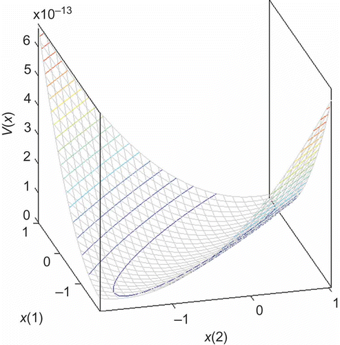
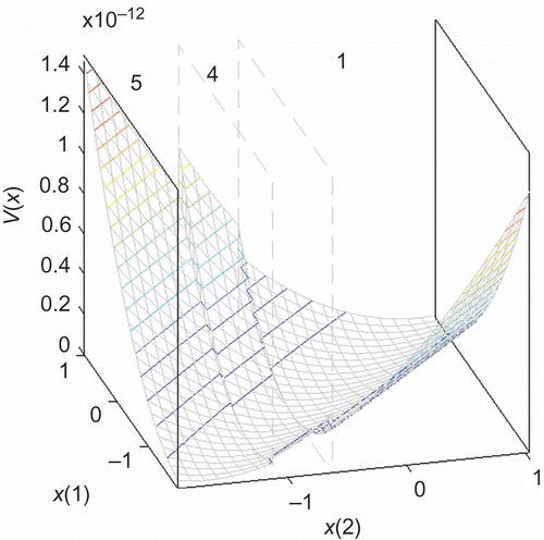
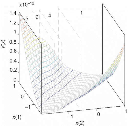
This section treats stability analysis using the common, the piecewise quadratic and the fuzzy Lyapunov approaches, all of which are extended by the decay rate $\alpha$. Basically, the decay rate is an important characteristic for the dynamic behaviour of a nonlinear system. It provides comparability between different Lyapunov approaches as well as between LMNs of different complexities which have been constructed from the same data set [11]. In this context, two cases must be distinguished:

• $\alpha$ is a constant: This case is analogous to the existing approaches and not the focus of this article. Exponential stability with a desired decay rate can be investigated instead of the asymptotic stability of the existing approaches.

• $\alpha$ is a decision variable: The problem of proving stability is extended by the question of how to find the extremal decay rate for a given system which amounts to finding the infimum of $\alpha$ under LMI constraints. This leads to generalized eigenvalue problems and requires a specific type of solver. The gevp solver of the MATLAB® Robust Control Toolbox™ (MathWorks, Natick, MA, USA) [39] is specialized in such problems and used for all stability investigations in this work. Other commonly used solvers such as feasp, mincx of MATLAB® Robust Control Toolbox™ [39], SeDuMi [40] and Sdpt-3 [41] cannot directly solve generalized eigenvalue problems.

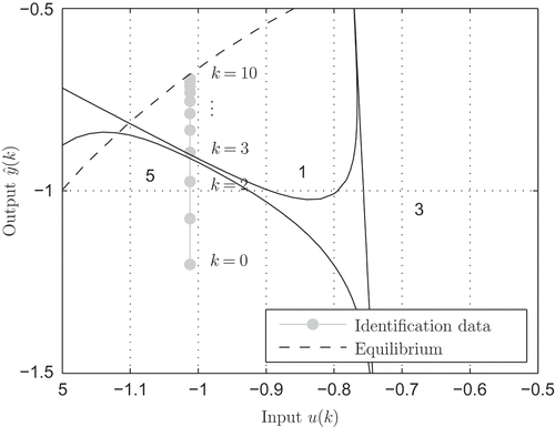
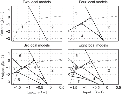
  By treating $\alpha$ as a decision variable, the achievable decay rate of different LMN variants and the various Lyapunov stability criteria can be used as a quantitative measure because different LMN variants or stability criteria will yield different maximum decay rates for the same system [11]. In this context, it is essential to keep in mind that for a specific input–output data set (system), arbitrary LMN variants exist and boundaries for provable stability may exist, too. To illustrate this situation, consider the example in Figure 4: Here, data from a nonlinear dynamic process are modelled by four different LMN variants.

  Figure 4. Contour plot of the validity functions of different LMN variants and the equilibrium (dashed line).

  

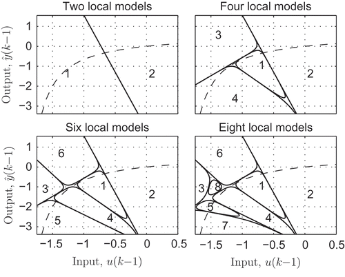
  One important bound is the maximum number of local models where a stability proof is still possible. This number is of particular interest because the approximation quality is usually increased by the number of local models, whereas a proof of stability becomes increasingly difficult as the number of local models grows [9]. Thus, it is possible to determine the best LMN variant in terms of stability and approximation quality for a given input–output data sequence. However, it is a versatile method to compare the different LMNs and Lyapunov stability criteria. The usual method to compare different Lyapunov approaches is to vary two system parameters (see e.g. [16,18,24]). Within this two-dimensional parameter space, a point-wise analysis of the provable stability region for different Lyapunov approaches is used. However, the proposed approach fits to the workflow of system identification because the system parameters of the local system matrices are determined from the identification process and thus fixed for stability analysis.

3.1. Lyapunov’s direct method

The stability of LMNs can be proved by Lyapunov’s direct method. This general approach is based on a state-space formulation of the system, such as (22), and one has to find a suitable Lyapunov function $V(\mathbf{x})$.

Definition 3.1.

A Lyapunov function basically has to satisfy four properties to provide global asymptotic stability of a system [7]:

1. $V(\mathbf{x}(k)=0)=0$

2. $V(\mathbf{x}(k))>0$ for $\mathbf{x}(k)\ne 0$

3. $V(\mathbf{x}(k))$ approaches infinity as $\parallel \mathbf{x}(k)\parallel \to \mathrm{\infty }$

4. $\mathrm{\Delta }V(\mathbf{x}(k))=V(k+1)-V(k)<0,\mathrm{\forall }k\in {\mathbb{N}}^{+}$.

Lemma 1.

For exponential stability, the Lyapunov function must satisfy (1–3) of Definition 3.1 and decrease strictly monotonically over time $k$ with a decay rate $\alpha ,\text{break}0<\alpha <1$:

(26) $V(k+1)-{\alpha }^{2}V(k)\le 0,\mathrm{\forall }k\in {\mathbb{N}}^{+}.$(26)

The proof of Lemma 1 is given in [42].

3.2. Common quadratic Lyapunov approach for discrete-time systems

The common quadratic Lyapunov approach was the first stability criterion to be proposed for LMNs [7]. It aims to find one common quadratic Lyapunov function

(27) $V(k)={\mathbf{x}}^T(k)\mathbf{P}\mathbf{x}(k)>0,\mathbf{P}\succ 0$(27)

for all local models, see Figure 5.

Figure 5. Common quadratic Lyapunov function.

Thus, the LMI solver has to find a single positive definite matrix and must simultaneously satisfy as many LMIs as there are local models. This usually leads to conservatism due to the fact that by increasing the number of local models, it will be more difficult to find a common Lyapunov function [25,38].

The common quadratic Lyapunov approach from [7; Theroem 4.2] is extended with the decay rate according to Lemma 1:

Theorem 1.

The dynamic LMN (22) is globally exponentially stable with the decay rate $\alpha$ if there exists a common positive definite matrix P for all local models:

(28) $\mathbf{P}\succ 0$(28)

such that the following conditions are satisfied:

(29) $\alpha =\inf \left\{0<\alpha <1:A_i^{T}P{A}_i\prec {\alpha }^{2}P\right\},\forall i\in I.$(29)

The proof of Theorem 1 directly follows from [7] and Lemma 1.

Remark 3.

The LMI solver minimizes $\alpha$ and calculates P under the LMI constraints (28) and (29) of Theorem 1 simultaneously. Thus, the resulting $\alpha$ can be seen as the infimum for the given problem.

In Theorem 1, a common matrix P must be found for all local system matrices ${\mathbf{A}}_i$. This is a much stronger condition than the individual stability of the local linear models, for which only ${\mathbf{A}}_i^T{\mathbf{P}}_i{\mathbf{A}}_i-{\mathbf{P}}_i\prec 0$ with individual ${\mathbf{P}}_i$ would be required, [29]. Note that it may not be possible to find a P that satisfies (29), although the global model may be asymptotically stable, [11, Section 4.2]. The condition (29) is therefore sufficient but not necessary.

3.3. Piecewise quadratic Lyapunov approach for discrete-time systems

The basic idea of this approach is the partitioning of the state space into subspaces $S_i$ which are defined using the validity functions of the local models. Thus, each local model defines a corresponding subspace. Within these subspaces, the local dynamics are characterized by the corresponding system matrix ${\mathbf{A}}_i$ of the local model with the additional disturbance term $\mathrm{\Delta }{\mathbf{A}}_i(\Phi )$ which describes the influence of interacting local models, see Equation (24). These disturbance terms have a particular meaning for the piecewise quadratic Lyapunov approach because they constitute so-called uncertainty terms $\mathrm{\Delta }{\mathbf{A}}_i^T(\Phi )\mathrm{\Delta }{\mathbf{A}}_i(\Phi )$ in the LMI [10]. For the purpose of stability analysis, the following upper bounds ${\mathbf{E}}_{iA}^T{\mathbf{E}}_{iA}$ for the uncertainty terms of the subspaces (24) are introduced:

(30) $\Delta A_i{(\Pi )}^T\Delta A_i(\Pi )E_{iA}^T{E}_{iA},\forall i\in I,$(30)

where the particular validity function vector $\Phi$ for which the equality sign of Equation (30) holds is a-priori unknown.

Remark 4.

The upper bounds of the uncertainty terms lead to conservatism of the resulting stability analysis [9,11], especially for the worst case bounds presented in [43,44]. Thus in [38,43,44], advanced methods are presented which approximate the upper bounds and lead to less conservatism. For systems with local dynamics in controllability canonical form an optimization based method is introduced in [38]. For switching systems with hard-limit validity functions, [12], and/or continuous time systems [13], the upper bounds of the uncertainty terms do not appear and the piecewise quadratic Lyapunov approach is less conservative as for discrete-time LMNs with overlapping validity functions.

To prove global stability, local quadratic Lyapunov functions have to be found for all subspaces, see Figure 6, which are linked by feasible transitions from one subspace into another. Consequently, the Lyapunov functions must decrease at each timestep, even if the state transits from one subspace into another to satisfy (26) [10].

Figure 6. Piecewise quadratic Lyapunov function.

Theorem 2 follows by extending [10; Theorem 3.1] with the decay rate according to Lemma 1:

Theorem 2.

The dynamic LMNs (22) and (24), respectively, are exponentially stable with decay rate $\alpha$ in the region

(31) $\mathcal{S}=\bigcup _{i\in \mathcal{I}}{S}_i,$(31)

which is the union of the subspaces $S_i$, if there exists a set of symmetric positive definite matrices ${\mathbf{P}}_i$:

(32) ${\mathbf{P}}_i\succ 0,\mathrm{\forall }i\in \mathcal{I}$(32)

such that the following conditions are satisfied:

(33) $\begin{array}{rl}\alpha =inf\left\{0<\alpha <1:\left[\begin{array}{cc}{\mathbf{A}}_i^T{\mathbf{P}}_j{\mathbf{A}}_i+\frac{1}{\epsilon }{\mathbf{E}}_{iA}^T{\mathbf{E}}_{iA}& {\mathbf{A}}_i^T{\mathbf{P}}_j\\ {\mathbf{P}}_j{\mathbf{A}}_i& {\mathbf{P}}_j-\frac{1}{\epsilon }\mathbf{I}\end{array}\right]\prec {\alpha }^2\left[\begin{array}{cc}{\mathbf{P}}_i& \mathbf{0}\\ \mathbf{0}& \mathbf{0}\end{array}\right]\right\},& \\ \\ \epsilon >0,\\ \mathrm{\forall }i\in \mathcal{I},j\in {\mathrm{\Omega }}_i^p,& \text{aeqnum}\end{array}$(33)

where the set ${\mathrm{\Omega }}_i^p$ denotes those local models where a transition from model $i$ is possible, that is,

(34) ${\mathrm{\Omega }}_i^p=\left\{j|(\tilde{\mathbf{x}}(k)\in S_i\wedge \tilde{\mathbf{x}}(k+1)\in S_j),j\in \mathcal{I}\right\},\mathrm{\forall }i\in \mathcal{I}.$(34)

The proof of Theorem 2 follows from [10] and Lemma 1.

Remark 5.

Equation (34) includes the case $i=j$, which requires that every local model must have stable dynamics as a necessary condition. The case $i\ne j$ requires that the piecewise Lyapunov function decreases when the system state transits across the region boundary from $S_i$ to $S_j$. To prove global stability, $\mathcal{S}$ has to cover the whole partition space.

Remark 6.

The gevp solver provided by MATLAB® Robust Control Tool box requires a positive definite matrix on the right hand side of (33). Thus (33) is reformulated to:

(35) $\alpha =inf\left\{0<\alpha <1:{\mathbf{Z}}_i⪯{\alpha }^2{\mathbf{P}}_i\right\}\mathrm{\forall }i\in \mathcal{I}$(35)

such that

(36) $\left[\begin{array}{cc}{\mathbf{A}}_i^T{\mathbf{P}}_j{\mathbf{A}}_i+\frac{1}{\epsilon }{\mathbf{E}}_{iA}^T{\mathbf{E}}_{iA}& {\mathbf{A}}_i^T{\mathbf{P}}_j\\ {\mathbf{P}}_j{\mathbf{A}}_i& {\mathbf{P}}_j-\frac{1}{\epsilon }\mathbf{I}\end{array}\right]\prec \left[\begin{array}{cc}{\mathbf{Z}}_i& \mathbf{0}\\ \mathbf{0}& \mathbf{0}\end{array}\right],\epsilon >0,\mathrm{\forall }i\in \mathcal{I},j\in {\mathrm{\Omega }}_i^p.$(36)

3.4. Fuzzy Lyapunov approach for discrete-time systems

The fuzzy Lyapunov approach [9,14–15,18–22,45–46] aims to find a non-quadratic Lyapunov function for the global model, see Figure 7,

(37) $V(k)={\mathbf{x}}^T(k)\left(\sum _{\mathcal{I}}{\mathrm{\Phi }}_i(\tilde{\mathbf{x}}(k)){\mathbf{P}}_i\right)\mathbf{x}(k)>0,$(37)

Figure 7. Fuzzy Lyapunov function.

with individual positive definite ${\mathbf{P}}_i$ matrices. Note that each local model independently satisfies (27) (there is an individual ${\mathbf{P}}_i$ matrix associated with each local model).

Remark 7.

The validity functions ${\mathrm{\Phi }}_i$ in (37) are equivalent to those of the local models in (22).

For asymptotic stability, all local models must be stable as a prerequisite. Furthermore, every possible trajectory must satisfy (5) of Definition (3.1). This shows that the feasible model transitions are of high interest when using the fuzzy Lyapunov approach. Theorem 3 follows by extending the Main Theorem of [14] with the decay rate according to Lemma 1:

Theorem 3.

The dynamic LMN is exponentially stable with the decay rate $\alpha$ in the region $U$ if there exists a set of positive definite matrices ${\mathbf{P}}_i$:

(38) $P_i\succ 0,\forall i\in I$(38)

such that the following conditions are satisfied:

(39) $\alpha =\inf \left\{0<\alpha <1:A_i^T{P}_j{A}_i\prec {\alpha }^2{P}_i\right\},\forall i\in I,j\in {\Omega }_i^f,$(39)

where the set ${\mathrm{\Omega }}_i^f$ defines all possible model transitions of model $i$ within region U [14]. By using the dominant region of a local model, according to (23), the possible transitions can be defined as

(40) $\begin{array}{rl}& {\mathrm{\Omega }}_i^f=\left\{j|(\tilde{\mathbf{x}}(k)\in S_i\wedge \tilde{\mathbf{x}}(k+1)\in S_j)\vee \right. \\ & \left. (\tilde{\mathbf{x}}(k)\in S_j\wedge \tilde{\mathbf{x}}(k+1)\in S_i),j\in \mathcal{I}\right\},\\ \mathrm{\forall }i\in \mathcal{I}\end{array}$(40)

and contain the model indices where a transition is possible from model $i$ to $j$ and from $j$ to $i$ within region U. This includes the case $i=j$ which requires that every local model must have stable dynamics as a necessary condition.

The proof of Theorem 3 follows from [14] and Lemma 1.

Remark 8.

The fuzzy Lyapunov approach requires that both directions of a transitions are considered. The reason is that the sum in (37) causes an additional sum in the decay condition of the Lyapunov approach (Definition 3.1, 4). To prove global stability, this opposite direction has to be considered.

Remark 9.

In recent years, the fuzzy Lyapunov approach was refined in several works, see [18–22,47,48]. These approaches have shown, that they are less conservative than previous approaches. However, this work aims to give an overview and the presented extension with the decay rate can also be applied to these approaches.

4. Transition determination

4.1. General

From the stability criteria discussed so far, it is evident that the number of LMIs to be satisfied is critical for the success to prove stability by using the piecewise-quadratic and the fuzzy Lyapunov approaches. The more interactions between local models exist, the more LMIs have to be satisfied, which in turn reduces the chance to successfully prove stability. Each transition requires one additional LMI for the piecewise quadratic Lyapunov approach, see (34), and two additional LMIs for the fuzzy Lyapunov approach, see (40). Thus, the difficulty of finding a suitable Lyapunov function is increased when additional model transitions are taken into account. Therefore, a proper determination of the feasible model transitions will help to reduce conservatism or even makes a stability proof of complex LMNs possible at all. Thus, in this section, a method for the determination of all feasible model transitions is proposed. For such a methodology, its applicability to as many partitioning strategies as possible, see Figure 2, and the type of validity function, see Figure 3, is important.

If no information about the model transitions is available, then transitions between all models must be taken into account:

(41) ${\mathrm{\Omega }}_i^q={\mathrm{\Omega }}_i^f=\mathcal{I},\mathrm{\forall }i\in \mathcal{I}.$(41)

The proposed methodology determines the possible transitions in a LMN by utilizing an optimally designed excitation data sequence. As a consequence, the stability region U in the present article is aimed to be identical to the convex hull of the used data sequence. In this context, the convex hull is defined by the input/output data points for all time instances. In contrast, most available stability criteria for LMNs aim to show unbounded global stability (e.g. [9,11]) which can become too expensive when only a certain part of the LMN describes the actual dynamic operating range of the process. Nevertheless, it can not be ruled out that outside of this hull, unnoticed transitions occur. However, for the design of controllers or observers, stability close to or beyond that boundary is of only limited interest.

It must be noted, nevertheless, that the characteristics of the excitation data significantly contribute to the effectiveness of the proposed method. This is not a severe disadvantage, because in data-driven models the range of the identification data is a priori defined as the area of interest (e.g. operating area) and usually design of experiments (DoE [26]) is employed. DoE deals with planning, conducting, analysing and interpreting controlled tests to efficiently determine system parameters of a physical system.

4.2. Methodology

The information about the model transitions for the LMN will be represented by a so-called transition matrix $\mathbf{\Xi }$. It is based on the excitation data sequence and the method to generate it will be described in the following.

The excitation signals ${\mathbf{u}}_{\mathcal{J}}(\mathcal{K})$, which are generated by a proper DoE [26] and the model output $\tilde{\mathbf{y}}(\mathcal{K})$, which is generated by simulating the process using the considered LMN with the excitation signal, are merged to a matrix

(42) $L(k)=\left[u_J\left(k-M\right)\tilde{y}\left(k-N\right)\right],\forall k\in K,L\in {ℝ}^{K\times O},$(42)

the rows of which correspond to the observation vector $\mathbf{z}(k)$. The ordered set for the samples of the data sequence is given by

(43) $\mathcal{K}=(k\in \mathbb{N}|1\le k\le K),$(43)

where $K$ is the number of samples. Those signals which are used as input arguments to the validity function form a subset of the data sequence. The choice of such a particular subset is strongly dependent on the system’s nonlinearities and is thus usually done by the user.

The input arguments to the validity function are denoted by $\tilde{\mathbf{L}}$ indicating that it is a sub-matrix of L

(44) $\tilde{\mathbf{L}}=\mathbf{L}(\mathcal{K},\tilde{\mathcal{O}}),\tilde{\mathbf{L}}\in {\mathbb{R}}^{K\times \tilde{O}},$(44)

the rows of which correspond to $\tilde{\mathbf{z}}(k)$. Consequently, the output of a validity function C can be formulated as

(45) $\mathbf{C}(\mathcal{K},\mathcal{I})={\mathrm{\Phi }}_{\mathcal{I}}(\tilde{\mathbf{L}}(\mathcal{K})),\mathbf{C}\in {\mathbb{R}}^{K\times I}.$(45)

When the state trajectory evolves over time and transits through different local models a matrix of indices of the two most dominant local models D (= local models with maximum $\mathrm{\Phi }$) can be generated in a similar way as L by using C:

(46) $\begin{array}{rl}& \mathbf{D}(k)=[\{i_1|\mathbf{C}(k,i_1)=max(\mathbf{C}(k,\mathcal{I}))\}\{i_2|\mathbf{C}(k,i_2)=max(\mathbf{C}(k,\mathcal{I}\mathrm{\setminus }{i}_1))\}],\\ & \mathrm{\forall }k\in \mathcal{K},\mathbf{D}\in {\mathbb{N}}^{K\times 2}.\end{array}$(46)

The matrices C and D inherently contain the relevant information required to determine the actual model transitions. They are used to generate the transition matrix $\mathbf{\Xi }$ which compactly describes possible local model transits. $\mathbf{\Xi }$ is a square matrix with boolean entries and has the following properties:

(47) $dim\mathbf{\Xi }=I\times I,$(47)

(48) $\mathbf{\Xi }({\xi }_r,{\xi }_c)\in \{0,1\},\mathrm{\forall }{\xi }_r,{\xi }_c\in \mathcal{I}.$(48)

The elements of $\mathbf{\Xi }$ can be interpreted as follows:

$\begin{array}{rl}\mathbf{\Xi }({\xi }_r,{\xi }_c)=& 1\mathrm{i}\mathrm{f}\mathrm{t}\mathrm{h}\mathrm{e}\mathrm{r}\mathrm{e}\mathrm{i}\mathrm{s}\mathrm{a}\mathrm{t}\mathrm{r}\mathrm{a}\mathrm{n}\mathrm{s}\mathrm{i}\mathrm{t}\mathrm{i}\mathrm{o}\mathrm{n}\mathrm{f}\mathrm{r}\mathrm{o}\mathrm{m}\mathrm{m}\mathrm{o}\mathrm{d}\mathrm{e}\mathrm{l}{\xi }_r\mathrm{t}\mathrm{o}{\xi }_c\\ & \mathrm{a}\mathrm{n}\mathrm{d}\mathrm{z}\mathrm{e}\mathrm{r}\mathrm{o}\mathrm{o}\mathrm{t}\mathrm{h}\mathrm{e}\mathrm{r}\mathrm{w}\mathrm{i}\mathrm{s}\mathrm{e}\end{array}$

To generate the transition matrix $\mathbf{\Xi }$ two steps are necessary:

1. Initialize $\mathbf{\Xi }$ as boolean identity matrix

   (49) $\mathbf{\Xi }={\mathbf{I}}_I$(49)

   The main diagonal entries which formally refer to an interaction of a local model with itself must be set to one since the piecewise quadratic and the fuzzy Lyapunov approaches require stable local models [9].

2. Set the feasible model transitions

   From Equation (46), the two most dominant local models are determined for each sample. A valid transition is detected whenever the dominant models change or when the validity functions do not change by means of Boolean algebra:

   (50) $\begin{array}{rl}& \mathbf{D}(k,1)=\mathbf{D}(k-1,2)\wedge \mathbf{D}(k,2)=\mathbf{D}(k-1,1)\vee ,\\ & \mathbf{C}(k,\mathcal{I})=\mathbf{C}(k-1,\mathcal{I})\wedge \mathbf{D}(k,\left\{1,2\right\})=\mathbf{D}(k-1,\left\{1,2\right\}),\mathrm{\forall }k\in \mathcal{K}.\text{aeqnum}\end{array}$(50)

   Condition (50) is examined for all rows of C and D, respectively. The detected transition directly follows when Equation (50) is true for some $k$ and the respective entry is set in the transition matrix:

   (51) $\mathbf{\Xi }(\mathbf{D}(k-1,1),\mathbf{D}(k,1))=1.$(51)

The sets ${\mathrm{\Omega }}_i^p$ and ${\mathrm{\Omega }}_i^f$ which define the model transitions for the piecewise quadratic Lyapunov (34) and the fuzzy Lyapunov approach (40), respectively, directly follow from $\mathbf{\Xi }$:

(52) ${\mathrm{\Omega }}_i^p=\{j|\mathbf{\Xi }(i,j)=1,\mathrm{\forall }j\in \mathcal{I}\},\mathrm{\forall }i\in \mathcal{I},$(52)

(53) ${\mathrm{\Omega }}_i^f=\{j|\mathbf{\Xi }(i,j)=1\vee \mathbf{\Xi }(j,i)=1,\mathrm{\forall }j\in \mathcal{I}\},\mathrm{\forall }i\in \mathcal{I}.$(53)

5. Simulation examples

In Section 5.1, a simple example exemplarily shows a single transition from one model to another. The effectiveness of the fuzzy Lyapunov approach in conjunction with the proposed method is demonstrated by means of an illustrative nonlinear process in Section 5.2.

5.1. Single transition

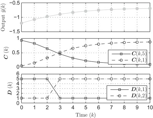
Figure 8 illustrates an exemplary trajectory of an identification data sequence with constant input $u(k)$ and the 50% contour lines of the validity functions of the local models. The timestep from $k=2$ to $k=3$ is considered in detail.

Figure 8. Trajectory within partition space.

The analysis of the trajectory by the method proposed in Section 4 is illustrated in Figure 9.

Figure 9. Validity sequence.

The upper plot of Figure 9 shows the system output over time, the middle one shows how the validity function outputs of local models 1 and 5 and the bottom one illustrates how the two most dominant models were determined by (51).

At $k=2$, local model $5$ is most dominant $(D(2,1)=5)$ and at $k=3$, $(D(3,1)=1)$, which indicates that model $1$ is now dominating:

(54) $\mathbf{D}(2,1)=5,\mathbf{D}(2,2)=1,\mathbf{D}(3,1)=1,\mathbf{D}(3,2)=5.$(54)

Thus, according to (50), a valid transition is detected and the corresponding entry is set in the transition matrix according to (51):

$\mathbf{\Xi }(5,1)=\mathbf{\Xi }(1,5)=1$

5.2. Nonlinear dynamic process

For illustrative purposes, the stability of a complex nonlinear dynamic process is investigated by using the presented Lyapunov approaches of Section 3 and using the transition determination of Section 4. By means of the decay rate, different LMN variants comprising different numbers of local models and the conservatism of the considered Lyapunov approaches are compared. Further, the influence of the transition determination is demonstrated.

The nonlinear dynamic process is adopted from [29,49] and is described by the following difference equation:

(55) $\begin{array}{rl}y(k)=& 0.133u(k-1)-0.0677u(k-2)+1.5y(k-1)\\ & -0.7y(k-2)+u(k)[0.1y(k-1)-0.2y(k-2)].\text{aeqnum}\end{array}$(55)

In this example, the input $u(k)$ is bounded to the interval $[-1.75,0.5]$.

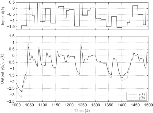
Figure 10 demonstrates that the system has weakly damped oscillatory behaviour for large inputs, whereas for small inputs strongly damped aperiodic behaviour is present.

Figure 10. Input and output of the process and the LMN.

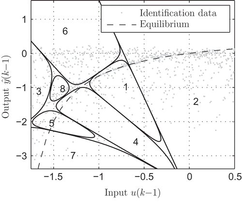
For system identification, an excitation signal was generated to capture both the nonlinear dynamic and static behaviour [26]. From these data, different LMNs comprising up to eight local models were generated by the algorithm presented in [30], where the local models are defined by an axis oblique decomposition of the partition space. Figure 11 shows a contour plot of the validity functions

(56) $\tilde{\mathbf{x}}(k)=[u(k-1)\hat{y}(k-1)]$(56)

Figure 11. Contour plot of the validity functions and identification data sequence.

as well as the identification data for the LMN with eight local models.

The partitioning strategy in [30] uses statistical methods to avoid overfitting by local models generated with only few observations. Figure 12 illustrates a contour plot of the validity functions of LMNs comprising 2, 4, 6 and 8 local models.

Figure 12. Contour plot of the validity functions of different LMN variants.

Figure 13 illustrates the different decay rates determined by the three investigated Lyapunov-based stability criteria depending on the number of local models. This example shows noteworthy results:

Figure 13. Minimum decay rate $\alpha$ of different stability criteria depending on the number of local models: common quadratic Lyapunov approach (black), fuzzy Lyapunov approach (dark grey), piecewise quadratic Lyapunov approach with upper bounds as in [38] (light grey) and piecewise quadratic Lyapunov approach without upper bounds (for comparison) (white).

• In all cases, the fuzzy Lyapunov approach achieves the lowest decay rate and thus is the least conservative (except the piecewise quadratic Lyapunov approach without the upper bounds). This agrees with the results of [9,11,14,25]. The piecewise quadratic Lyapunov approach without the upper bounds is just included to show the influence of the upper bounds. For LMNs with switching validity functions, where the system parameters switch hard during a model transition, the upper bounds do not appear. Thus, the LMN without the upper bounds has the same local system parameters and the partition space but differs in the validity function.

• There is no monotonic behaviour of the different decay rates as the number of local modes is increased. This is due to fact that the difficulty of finding a suitable Lyapunov function mainly depends on the local dynamics and the number of LMIs. By increasing the number of local models, the variety of the different local dynamics gradually decreases and the number of LMIs of the stability criteria are increased at the same time.

  The LMNs with less than four models are a coarse approximation of the process. This leads to strongly different dynamics of the local models and thus to high conservatism. The decrease of the conservatism observed when the number of local models is increased from four to six local models can be attributed to the reduced differences of the local system dynamics (compare Figure 13). For more than six models, the decay rate is increased in all approaches. However, it is shown that the LMNs with five to eight local models are exponentially stable. Furthermore, for controller design, the decay rate can be used to indicate the optimal number of local models and consequently the number of local controllers. In this case, the LMN with six local models would be the best option because it has the smallest decay rate.

• There is a strong influence of the upper bounds to the conservatism of the piecewise quadratic Lyapunov approach (compare light-grey and white of Figure 13). This general relationship was already mentioned in [9,11,38,43]. Figure 13 further shows that the influence of the upper bounds is more dominant than the influence of the piecewise quadratic Lyapunov approach itself.

Using the algorithm presented in Section 4, the following model transitions (see (34) and (40)) are determined for the LMN comprising eight local models:

(57) $\begin{array}{rl}& {\mathrm{\Omega }}_1^p=\{1,2,6\},{\mathrm{\Omega }}_2^p=\{1,2\},\\ & {\mathrm{\Omega }}_3^p=\{3,5,8\},{\mathrm{\Omega }}_4^p=\{1,2,4,5,6\},\\ & {\mathrm{\Omega }}_5^p=\{4,5,7\},{\mathrm{\Omega }}_6^p=\{1,3,4,6,8\},\\ & {\mathrm{\Omega }}_7^p=\{4,5,7\},{\mathrm{\Omega }}_8^p=\{4,5,8\},\end{array}$(57)

(58) $\begin{array}{rl}& {\mathrm{\Omega }}_1^f=\{1,2,4,6\},{\mathrm{\Omega }}_2^f=\{1,2,4\},\\ & {\mathrm{\Omega }}_3^f=\{3,5,6,8\},{\mathrm{\Omega }}_4^f=\{1,2,4,5,6,7,8\},\\ & {\mathrm{\Omega }}_5^f=\{3,4,5,7,8\},{\mathrm{\Omega }}_6^f=\{1,3,4,6,8\},\\ & {\mathrm{\Omega }}_7^f=\{4,5,7\},{\mathrm{\Omega }}_8^f=\{3,4,5,6,8\}.\end{array}$(58)

Using (57) for the piecewise quadratic Lyapunov approach, the number of LMIs in (33) can be reduced from 64 to 27. Using (58) for the fuzzy Lyapunov approach, the number of LMIs in (39) can be reduced from 64 to 36.

Figure 14 illustrates the influence of the transition determination method of Section 4 by means of the fuzzy Lyapunov approach.

Figure 14. Minimum decay rate $\alpha$ of the fuzzy Lyapunov approach depending on the considered transitions: transition determination (58) (black), all transitions (41) (white).

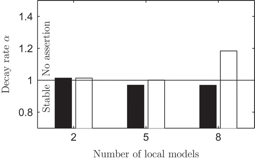
Figure 14 shows that the potential to reduce the conservatism is increased by the number of local models. The transition determination cannot reduce the conservatism of an LMN with only two local models because there is no possibility to reduce the number of LMIs. For five local models, a small but significant reduction in the transitions is achieved. Considering the LMN with eight local models, it is apparent that a stability check without proper transition determination does not allow for an assertion.

5.3. Results

Generally, the fuzzy Lyapunov approach shows the best results in most cases, especially when the information of the transition determination is used. There is a significant influence of the upper bounds on the conservatism of the piecewise quadratic Lyapunov approach, especially for LMNs from system identification. Thus, there is further potential to determine these upper bounds. Especially for switching systems, the piecewise quadratic Lyapunov approach demonstrates its strength.

Basically, there is a general trend that the conservatism is increased by the number of local models, see Figure 13. Nevertheless, the result of the nonlinear dynamic process shows that an increase in the local models may decrease the conservatism in particular cases, see models four to six of Figure 13.

6. Conclusion

A method for the quantitative comparison of LMNs and different Lyapunov approaches has been proposed in this article. For this purpose, three basic Lyapunov approaches were extended by the decay rate which provides a scalar stability measure. The presented concept helps to generate globally stable LMNs which are as accurate as possible or find the optimal number of local models for controller design. The introduced concept where the Lyapunov approach is extended by the decay rate can be easily adopted for most of the existing approaches. Further, a method was introduced which determines the model transitions by means of the identification data sequence. This transition determination method significantly reduces the conservatism of the piecewise quadratic and the fuzzy Lyapunov approach. A simulation example has been used to illustrate the influence of the numbers of local models on Lyapunov stability criteria as well as their inherent conservatism and the influence of the transition determination method presented in this article.

Acknowledgement

This work was supported by Christian Doppler Research Association and AVL List GmbH.

References

- R. Gao, Local model network application in control, Thesis, Dublin Institute of Technology, 2004.
- G. Gregorcic and G. Lightbody, Local model network identification with Gaussian processes, IEEE Trans. Neural Netw. 18 (2007), pp. 1404–1423.
- J. Novak and V. Bobal, Predictive Control of the Heat Exchanger Using Local Model Network, Proceedings of the 17th Mediterranean Conference on Control & Automation, IEEE, 2009, pp. 657–662.
- S. Jakubek and C. Hametner, Identification of neurofuzzy models using GTLS parameter estimation, IEEE Trans. Syst. Man Cybern. B Cybern. 39 (2009), pp. 1121–1133.
- R. Murray-Smith and T.A. Johansen, Multiple Model Approaches to Modelling and Control, Taylor & Francis, London, 1997.
- C. Hametner, C. Mayr, and S. Jakubek, Dynamic NOx emission modelling using local model networks [in revision], Int. J. Engine Res.
- K. Tanaka and M. Sugeno, Stability analysis and design of fuzzy control systems, Fuzzy Sets Syst. 45 (1992), pp. 135–156.
- A. Lyapunov, The general problem of the stability of motion, Int. J. Control. 55 (1992), pp. 531–773.
- G. Feng, A survey on analysis and design of model-based fuzzy control systems, IEEE Trans. Fuzzy Syst. 14 (2006), pp. 676–697.
- G. Feng, Stability analysis of discrete-time fuzzy dynamic systems based on piecewise Lyapunov functions, IEEE Trans. Fuzzy Syst. 12 (2004), pp. 22–28.
- G. Feng, Analysis and Synthesis of Fuzzy Control Systems, A Model Based Approach, CRC press, Taylor & Francis, Boca Raton, FL, 2010.
- M. Johansson and A. Rantzer, Computation of piecewise quadratic Lyapunov functions for hybrid systems, IEEE Trans. Automat. Contr. 43 (1998), pp. 555–559.
- M. Johansson and A. Rantzer, Piecewise quadratic stability of fuzzy systems, IEEE Trans. Fuzzy Syst. 7 (2000), pp. 713–722.
- Y. Wang, Z. Sun, and F. Sun, Stability Analysis and Control of Discrete-time Fuzzy Systems: A Fuzzy Lyapunov Function Approach, Proceedings of the 5th Asian Control Conference, IEEE, 2004.
- C. Sun, Y. Su, and C. Chuang, Relaxed Stabilization Criterion for TS Fuzzy Discrete System, Kainan University, Taiwan, 2009.
- E. Kim and H. Lee, New approaches to relaxed quadratic stability condition of fuzzy control systems, IEEE Trans. Fuzzy Syst. 8 (2000), pp. 523–534.
- E. Kim, D. Kim, and S. Analysis, Synthesis for an affine fuzzy system via LMI and ILMI: discrete case, IEEE Trans. Syst. Man Cybern. B Cybern. 31 (2001), pp. 132–140.
- T.M. Guerra, A. Kruszewski, and M. Bernal, Control law proposition for the stabilization of discrete Takagi–Sugeno models, IEEE Trans. Fuzzy Syst. 17 (2009), pp. 724–731.
- T. Guerra and L. Vermeiren, LMI-based relaxed nonquadratic stabilization conditions for nonlinear systems in the Takagi-Sugeno’s form, Automatica 40 (5) (2004), pp. 823–829.
- B. Ding, H. Sun, and P. Yang, Further studies on LMI-based relaxed stabilization conditions for nonlinear systems in Takgi-Sugeno’s form, Automatica 402 (3) (2006), pp. 503–508.
- A. Kruszewski, R. Wang, and T.M. Guerra, Nonquadratic stabilization conditions for a class of uncertain nonlinear discrete time TS fuzzy models: a new approach, IEEE Trans. Automat. Contr. 53 (2008), pp. 606–611.
- S. Zhou, J. Lam, and A. Xue, H-∞ filtering of discrete-time fuzzy systems via basis-dependent Lyapunov function approach, Fuzzy Sets Syst. 158 (2007), pp. 180–193.
- G. Gregorcic and G. Lightbody, Nonlinear system identification: from multiple-model networks to Gaussian processes, Eng. Appl. Artif. Intell. 21 (2008), pp. 1035–1055.
- H.-K. Lam and F.H.-F. Leung, Stability Analysis of Fuzzy-Model-Based Control Systems, Springer-Verlag, New York, 2011.
- C. Mayr, C. Hametner, M. Kozek, and S. Jakubek, Relaxed Fuzzy Lyapunov Approach for Dynamic Local Model Networks, Proceedings of the 2011 IEEE International Conference on Fuzzy Systems, Christian Doppler Laboratory for Model Based Calibration Methodologies, Vienna University of Technology, 2011.
- G.C. Goodwin and R.L. Payne, Dynamic system identification: experiment design and data analysis, Math. Sci. Eng. 136 (1977), p. 291.
- C. Hametner and S. Jakubek, New Concepts for the Identification of Dynamic Takagi-Sugeno Fuzzy Models, IEEE Conference on Cybernetics and Intelligent Systems, IEEE, 2006, pp. 185–190.
- O. Nelles and R. Isermann, Basis Function Networks for Interpolation of Local Linear Models, Proceedings of the 35th Conference on Decision and Control 1, IEEE, 1996, pp. 470–475.
- O. Nelles, Nonlinear System Identification: From Classical Approaches to Neural Networks and Fuzzy Models, Springer Verlag, Berlin, Heidelberg, 2001.
- C. Hametner and S. Jakubek, Neuro-Fuzzy Modelling Using a Logistic Discriminant Tree, Proceedings of the 2007 American Control Conference, IEEE, 2007, pp. 864–869.
- L. Breiman, Hinging hyperplanes for regression, classification, and function approximation, IEEE Trans. Inform. Theory 39 (1993), pp. 999–1013.
- S. Jakubek, N. Keuth, and A. Local Neuro-Fuzzy, Network for high-dimensional models and optimization, Eng. Appl. Artif. Intell. 19 (2006), pp. 705–717.
- O. Nelles, Local Linear Model Trees for On-Line Identification of Time-Variant Nonlinear Dynamic Systems, International Conference on Artificial Neural Networks, Springer, Berlin, Heidelberg, 1996.
- L. Thanh Ngo, L. Pham The, P. Hoang Nguyen, and K. Hirota, On Approximate Representation of Type-2 Fuzzy Sets Using Triangulated Irregular Network, Volume 4529, Foundations of Fuzzy Logic and Soft Computing, Springer, Berlin, Heidelberg, 2007.
- B. Hartmann, O. Banfer, O. Nelles, A. Sodja, L. Teslic, and I. Skrjanc, Supervised hierarchical clustering in fuzzy model identification, IEEE Trans. Fuzzy Syst. 19 (2011), pp. 1163–1176.
- J. Causa, G. Karer, A. Núñez, D. Sáez, I. Skrjanc, and B. Zupancic, Hybrid fuzzy predictive control based on genetic algorithms for the temperature control of a batch reactor, Comput. Chem. Eng. 32 (2008), pp. 3254–3263.
- P. Van Overschee, B. De Moor, and D. N4SI, Subspace algorithms for the identification of combined deterministic-stochastic systems, Automatica 30 (1994), pp. 75–93.
- C. Mayr, C. Hametner, M. Kozek, and S. Jakubek, Piecewise Quadratic Stability Analysis for Local Model Networks, Proceedings of the 2011 IEEE Multi-conference on System and Control, Christian Doppler Laboratory for Model Based Calibration Methodologies, Vienna University of Technology, 2011.
- Y. Nesterov and A. Nemirovskii, Interior-Point Polynomial Algorithms in Convex Programming, Theory and Application, Society for Industrial Mathematics, Philadelphia, siam ed., 1994.
- J. Sturm, Using SeDuMi 1. 02, a MATLAB toolbox for optimization over symmetric cones, Optim. Methods Softw. 11–12 (1999), pp. 625–653.
- K. Toh and M. Todd, SDPT 3- A MATLAB software package for semidefinite programming, Optim. Methods Softw. 11 (1999), pp. 545–581.
- M. Bernal and P. Husek, Non-quadratic performance design for Takagi-Sugeno fuzzy systems, Int. J. Appl. Math. Comput. Sci. 15 (2005), pp. 383–391.
- S. Cao, N. Rees, and G. Feng, Quadratic stability analysis and design of continuous-time fuzzy control systems, Int. J. Syst. Sci. 27 (1996), pp. 193–203.
- S. Cao, Analysis and design for a class of complex control systems part II: fuzzy controller design, Automatica 33 (1997), pp. 1029–1039.
- K. Tanaka, T. Hori, H. Wang, and A. Multiple Lyapunov, Function approach to stabilization of fuzzy control systems, IEEE Trans. Fuzzy Syst. 11 (2003), pp. 582–589.
- S. Zhou, G. Feng, J. Lam, and S. Xu, Robust H-∞ control for discrete-time fuzzy systems via basis-dependent Lyapunov functions, Inform. Sci. 174 (2005), pp. 197–217.
- S. Zhou, J. Lam, and W.X. Zheng, Control design for fuzzy systems based on relaxed nonquadratic stability and H Performance Conditions, IEEE Trans. Fuzzy Syst. 15 (2007), pp. 188–199.
- H.-N. Wu, Delay-dependent stability analysis and stabilization for discrete-time fuzzy systems with state delay: a fuzzy Lyapunov-Krasovskii functional approach, IEEE Trans. Syst. Man Cybern. B Cybern. 36 (2006), pp. 954–962.
- I. Leontaritis and S. Billings, Input-output parametric models for nonlinear systems part I: deterministic non-linear systems, Int. J. Control. 41 (1985), pp. 303–328.