Investigation of two-warehouse inventory problems in interval environment under inflation via particle swarm optimization

ABSTRACT

In this paper, a two-warehouse inventory problem has been investigated under inflation with different deterioration effects in two separate warehouses (rented warehouse, RW, and owned warehouse, OW). The objective of this investigation is to determine the lot-size of the cycle of the two-warehouse inventory system by minimizing the average cost of the system. Considering different inventory policies, the corresponding models have been formulated for linear trend in demand and interval valued cost parameters. In OW, shortages, if any, are allowed and partially backlogged with a variable rate dependent on the duration of the waiting time up to the arrival of the next lot. The corresponding optimization problems have been formulated as non-linear constrained optimization problems with interval parameters. These problems have been solved by an efficient soft computing method, viz. practical swarm optimization. To illustrate the model, a numerical example has been solved with different partially backlogging rates. Then to study the effect of changes of different system parameters on the optimal policy, sensitivity analyses have been carried out graphically by changing one parameter at a time and keeping the others at their original values. Finally, a fruitful conclusion has been reached regarding the selection of an appropriate inventory policy of the two-warehouse system.

KEYWORDS:

• Inventory
• two-warehouse
• deterioration
• partial backlogging
• inflation
• time-dependent demand
• particle swarm optimization

1. Introduction

It is commonly observed that the ever-increasing competition in the modern business scenario necessitates organizations to keep the provision of hiring an additional storage space despite the existence of their own warehouse. Due to several factors, like limited capacity of owned warehouse (OW) in an important marketplace, higher reordering cost, seasonal product, inflation-induced demand and price discount for bulk purchase, the inventory managers are bound to place the order for purchasing of an item more than the OW capacity. Generally, for storing the excess units purchased, an additional storage space is hired on a rental basis. Typically, this warehouse is known as rented warehouse (RW).

Over the last few decades, a number of researchers from different corners of the globe explored the area of two-warehouse inventory problems. For storing the goods purchased in excess of the capacity of OW, the wholesalers as well as the retailers generally resort to RW because reconstruction of a new warehouse for the said purpose may be much expensive. In this area, Hartely [1] first reported the concept of the two-warehouse inventory model in his book ‘Operations Research: A Managerial Emphasis’. After Hartely [1], a number of works have been carried out in this area. In this connection, one may refer to the recent works of Das, Maiti and Maiti [2], Niu and Xie [3], Rong, Mahapatra and Maiti [4], Jaggi et al. [5] and others.

In most of the inventory models of the existing literature of inventory control system, it is assumed that the lifetime of an item is infinite while it is in storage. This means that an item once in stock remains unchanged and fully usable for satisfying future demand. In practice, this assumption is not always true due to the effect of deterioration in the preservation of commonly used physical goods like wheat, paddy or any other type of foodgrains, vegetables, fruits, drugs, pharmaceuticals, etc. As a result, the loss due to this natural phenomenon (i.e., the deterioration effect) cannot be ignored in the analysis of the inventory system. Ghare and Schrader [6] first developed an inventory model for exponentially decaying inventory. Ghare and Schrader [6] first proposed an inventory model with constant deterioration rate. Covert and Philip [7] further extended and modified this model by considering variable deterioration rate. Shah [8] proposed a generalized economic order quantity (EOQ) model with variable deterioration rate and the allowance of complete backlogging of the unsatisfied demand. After a few years, a no-shortage inventory model for deteriorating item with time proportional demand was proposed by Sachan [9]. In the mean time, Kang and Kim [10] studied the deteriorating inventory systems dependent on price and production level. Since then, several researchers have explored the different aspects of inventory management for deteriorating item. In this regard, the recent works of Bhunia and Shaikh [11,12], Jaggi et al. [5], Bhunia et al. [13], Bhunia and Shaikh [14], Chung et al. [15] and We et al. [16] are worth mentioning.

In real-life situations, different factors like inflation and time value of money are seen to have a crucial impact on the inventory policy decisions. With the consideration of single inflation rate for all the associated costs, Buzacott [17] proposed some inventory models. After two years, Bierman and Thomas [18] developed an EOQ model with the incorporation of the effect of inflation and time value of money. Vrat and Padmanabhan [19] developed an EOQ model for deteriorating item with stock-dependent consumption rate and exponential decay. Datta and Pal [20] proposed an inventory model with linear time-dependent demand rate and shortages by considering the effects of inflation and time value of money. Wee and Law [21] developed inventory models for deteriorating item by taking into account the time value of money. In addition to these, researchers like Yang, Teng and Chern [22], Jaggi, Aggarwal and Goel [23], Hsieh, Dye and Ouyang [24], Dey, Mondal and Maiti [25], Jaggi et al. [5] and others have also contributed to this field of research.

A few years back, considering two alternative situations a two-warehouse inventory model with constant demand rate for deteriorating item under inflation was proposed by Yang [26]. In the first situation, the inventory system starts with an instant order and ends with shortages, whereas in the second situation, the system begins with shortages and ends without shortages. After two years, Yang [27] extended these models with the incorporation of partial backlogging. Further, the two alternative situations were compared by following the minimum cost approach. Recently, Jaggi et al. [5] proposed an inventory model by considering a linear time-dependent demand rate for deteriorating item, inflation and partial backlogging rate in a two-warehouse system.

This paper deals with an interval-oriented inventory model for linear trend in demand under inflationary condition with different deterioration rates in two separate warehouses (RW and OW) considering two different policies (inventory follows shortage (IFS) and shortage follows inventory (SFI)) and interval valued cost parameters (holding cost, shortage cost and ordering cost). The replacement rate is infinite. The stocks in RW are transferred to OW in a continuous release pattern and the associated transportation cost is taken into account. In OW, shortages, if any, are allowed and partially backlogged with a rate dependent on the duration of the waiting time up to the arrival of the next lot. The objective of this work is to select the better inventory policy for finding the optimal lot-size by minimizing the average cost of the system. The corresponding problems have been formulated as non-linear constrained optimization problems with interval parameters, which have been solved by an efficient soft computing method, viz. particle swarm optimization (PSO). Then, to illustrate the model, we have solved a numerical example with different partially backlogging rates. Finally to study the effect of changes of different system parameters on the initial stock level of the stock-in period, maximum shortage level along with the best found cost of the system, sensitivity analyses have been carried out graphically by changing one parameter at a time and keeping the others at their original values.

2. Assumptions and notations

The following notations and assumptions are used in this paper.

Assumptions:

• (i) Replenishment rate is infinite and lead-time is constant.

• (ii) The OW has a fixed capacity and the RW has unlimited capacity.

• (iii) The inventory costs (including holding cost and deterioration cost) are interval valued and the costs in RW are higher than those in OW.

• (iv) The inventory planning horizon is infinite and the inventory system involves only one item.

• (v) Deterioration is counted when the quantities are stored in both the warehouses. Deteriorated units are fully rejected during the inventory cycle.

• (vi) Shortages, if any, are allowed and partially backlogged. During the stock-out period the backlogging rate is dependent on the length of the waiting time up to the arrival of fresh lot. Considering this situation the backlogging rate is denoted by, $\theta \left(t\right)$ which is a differentiable and decreasing function of time t with $0\le \theta (t)\le 1,\theta (0)=1$ and $\underset{t\to \mathrm{\infty }}{lim}\theta (t)=0.$ It is to be noted that if $\theta (t)=1$for all t, then shortages are completely backlogged.

Notations:

For inventory models:

Table

$f\left(t\right)$	Demand rate dependent linearly on time t, i.e., $f\left(t\right)=a+bt$ where $a,b>0$
IFS	Inventory follows shortage
SFI	Shortage follows inventory
$S$	Highest stock level at the beginning of stock-in period
R	Highest shortage quantity due to partial backlogging
$L_1$-system	Single-warehouse system
$L_2$-system	Two-warehouse system
W	Storage capacity of OW
$\theta \left(t\right)$	Backlogging rate, which is a function of waiting time t
$\alpha ,\beta$	Deterioration rates in both warehouses OW and RW, respectively ($0<\alpha ,\beta <<1$)
r	Rate of inflation
$C_o=[C_{oL},C_{oR}]$	Interval valued inventory ordering cost per order
$C_p=[C_{pL},C_{pR}]$	Interval valued inventory purchasing cost per unit
$C_{ho}=[C_{hoL},C_{hoR}]$	Interval valued inventory holding cost per unit per unit time in OW
$C_{hr}=[C_{hrL},C_{hrR}]$	Interval valued inventory holding cost per unit per unit time in RW
$C_b=[C_{bL},C_{bR}]$	Interval valued inventory backlogging cost over the entire cycle per unit per unit time
$C_{ls}$=$[C_{lsL},C_{lsR}]$	Interval valued inventory opportunity cost due to lost sales
$TC{2}^{(1)}$,$TC{2}^{(2)}$	Present value of the total relevant costs per unit time in IFS and SFI policies, respectively, for two-warehouse inventory system
$TC{1}^{(1)}$,$TC{1}^{(2)}$	Total relevant costs per unit time in IFS and SFI policies, respectively, for single-warehouse system
$TC{W}^{(1)}$,$TC{W}^{(2)}$	Boundary costs in IFS and SFI policies, respectively, for single-warehouse system
$I_o\left(t\right),I_r(t)$	Inventory levels in OW and RW, respectively, at time t
$t_r$	Time at which the inventory level reaches zero in RW
$t_o$	Time at which the inventory level reaches zero in OW ($t_o>t_r$)
$t_s$	Time at which the shortage level reaches the lowest point in the replenishment cycle
T	Inventory cycle length
For PSO:
p_size	Population size
m_gen	Maximum number of generations
$\chi$	Constriction factor
$c_1\left(>0\right)$	Cognitive learning rate
$c_2\left(>0\right)$	Social learning rate
$r_1$, $r_2$	Uniformly distributed random numbers lying in the interval [0, 1].
${v_i}^{(k)}$	Velocity of the i-th particle at the k-th generation/iteration
${x_i}^{(k)}$	Position of the i-th particle of population at the k-th generation
$p_i^{(k)}$	Best previous position of the i-th particle at the k-th generation
$p_g^{(k)}$	Position of the best particle among all the particles in the population

3. Interval mathematics

In the proposed inventory models, different inventory costs are considered as interval numbers. So to handle those numbers, interval mathematics, interval functions, interval order relations and central tendencies of interval numbers are essential in the formulation of the models.

An interval number A can be defined as A = [a_L, a_R] = $\{x:{\mathrm{a}}_{\mathrm{L}}\le x\le a_R,x\in \mathrm{R}\}$ of width (a_{R –} a_L). Every real number $x\in R$ can be expressed as a degenerate interval number [x, x] with zero width. An interval number can also be expressed in the form of centre and radius of the interval as $A=[a_C,a_W]$=$\left\{x:a_C-a_W\le x\le a_C+a_W,x\in R\right\}$, where a_C = (a_L + a_R)/2 = centre of the interval and a_W = (a_R – a_L)/2 = radius of the interval. The details about the definitions of the first four operations (addition, subtraction, multiplication and division) of two interval numbers are given in Moore et al. [28].

Again according to Karmakar et al. [29], the modulus of an interval can be defined as follows:

$\left|A\right|=\left|\left[a_L,a_R\right]\right|=\left\{\begin{array}{c}\left[a_L,a_R\right]\mathrm{i}\mathrm{f}{a}_L\ge 0\\ \left[\left|a_R\right|,\left|a_L\right|\right]\mathrm{i}\mathrm{f}{a}_R\le 0\\ \left[0,\left|a_L\right|\right]\mathrm{i}\mathrm{f}{a}_L<0,\hspace{0.17em}{a}_R>0& \&\left|a_L\right|\ge \left|a_R\right|\\ \left[0,\hspace{0.17em}\left|a_R\right|\right]\mathrm{i}\mathrm{f}{a}_L<0,\hspace{0.17em}{a}_R>0& \&\left|a_L\right|<\left|a_R\right|.\end{array}\right)$

3.1. Functions of finite interval

Some important functions such as exponential, logarithmic functions of interval arguments are expressed in the form of interval as follows:

(i) $exp(A)=exp([a_L,a_R])=[exp(a_L),exp(a_R)].$

(ii) $log(A)=log([a_L,a_R)]=[log(a_L),log(a_R)],$ provided $a_L>0.$

3.2. Interval order relations

Let $A=[a_L,a_R]$ and $B=[b_L,b_R]$ be two intervals. Then these two intervals may be any one of the following types:

Type-1: Two intervals are disjoint.

Type-2: Two intervals are partially overlapping.

Type-3: One of the intervals contains the other one.

Recently Sahoo et al. [30] proposed the revised definitions of order relations between two interval numbers corresponding to maximization and minimization problems. These definitions are as follows:

Definition-1: The order relation ${>}_{max}$ between the intervals $A=[a_L,a_R]=⟨a_c,a_w⟩$ and $B=[b_L,b_R]=⟨b_c,b_w⟩$, then for maximization problems

(i) $A{>}_{max}B\iff a_c>b_c\mathrm{f}\mathrm{o}\mathrm{r}\mathrm{T}\mathrm{y}\mathrm{p}\mathrm{e}\mathrm{I}\mathrm{a}\mathrm{n}\mathrm{d}\mathrm{T}\mathrm{y}\mathrm{p}\mathrm{e}\mathrm{I}\mathrm{I}\mathrm{i}\mathrm{n}\mathrm{t}\mathrm{e}\mathrm{r}\mathrm{v}\mathrm{a}\mathrm{l}\mathrm{s},$

(ii) $A{>}_{max}B\iff$ either $a_c\ge b_c\wedge a_w<b_w$or $a_c\ge b_c\wedge a_R>b_R\mathrm{f}\mathrm{o}\mathrm{r}\mathrm{T}\mathrm{y}\mathrm{p}\mathrm{e}\mathrm{I}\mathrm{I}\mathrm{I}\mathrm{i}\mathrm{n}\mathrm{t}\mathrm{e}\mathrm{r}\mathrm{v}\mathrm{a}\mathrm{l}\mathrm{s},$

According to this definition, the interval$A$ is accepted for maximization case. Clearly, the order relation $A{>}_{max}B$ is reflexive and transitive but not symmetric.

Definition-2: The order relation ${<}_{min}$ between the intervals $A=[a_L,a_R]=⟨a_c,a_w⟩$ and $B=[b_L,b_R]=⟨b_c,b_w⟩$, then for minimization problems

(i) $A{<}_{min}B\iff a_c<b_c\mathrm{f}\mathrm{o}\mathrm{r}\mathrm{T}\mathrm{y}\mathrm{p}\mathrm{e}\mathrm{I}\mathrm{a}\mathrm{n}\mathrm{d}\mathrm{T}\mathrm{y}\mathrm{p}\mathrm{e}\mathrm{I}\mathrm{I}\mathrm{i}\mathrm{n}\mathrm{t}\mathrm{e}\mathrm{r}\mathrm{v}\mathrm{a}\mathrm{l}\mathrm{s},$

(ii) $A{<}_{min}B\iff$ either $a_c\le b_c\wedge a_w<b_w$or $a_c\le b_c\wedge a_L<b_L\mathrm{f}\mathrm{o}\mathrm{r}\mathrm{T}\mathrm{y}\mathrm{p}\mathrm{e}\mathrm{I}\mathrm{I}\mathrm{I}\mathrm{i}\mathrm{n}\mathrm{t}\mathrm{e}\mathrm{r}\mathrm{v}\mathrm{a}\mathrm{l}\mathrm{s}.$

According to this definition, the interval$A$ is accepted for minimization case. Clearly, the order relation $A{<}_{min}B$ is reflexive and transitive but not symmetric.

4. The proposed models

The goal of this work is to develop and also to solve the inventory models in interval environment considering both IFS and SFI policies for determining the lot-size by minimizing the average cost of the system.

4.1. Two-warehouse model with SFI policy

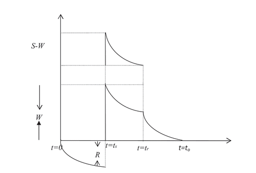
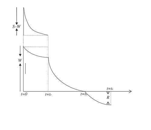
This model considers shortage first and ends without shortage. Initially (i.e., at time t = 0), shortages start to occur with a rate $\theta (t_s-t)$ and continue up to the time $t=t_s$. At time $t=t_s$, (S +R) units of item are replenished by the supplier. After fulfilling partially backlogged quantities, the on-hand inventory level is S units. Out of S units, W units are kept in OW and the remaining (S-W) units are stored in RW. The inventory level of (S-W) units in RW is depleted gradually in the interval $t_s\le t\le t_r$ for meeting the demand of customers and deterioration effect of the item and it reaches zero at $t=t_r$. During this time, the inventory level W in OW also reduces due to the effect of deterioration. Inventory level in OW decreases during the period $t_r\le t\le t_o$ due to demand and deterioration simultaneously, and at time $t=t_o(=T),$ the inventory level reaches zero. The pictorial representation of this policy is shown in Figure 1.

Figure 1. Pictorial representation of two-warehouse inventory system with SFI policy.

The stock is depleted gradually at RW during $t_s\le t\le t_r$ mainly to meet the demand by the customers and partly due to the deterioration effect of the item, which are disposed continuously as they approach the selling point. Hence the inventory level $I_r\left(t\right)$ at RW satisfies the following differential equation:

(1) $\frac{d{I}_r\left(t\right)}{dt}+\beta I_r\left(t\right)=-f\left(t\right),t_s\le t\le t_r$(1)

with the condition

(2) $I_r\left(t\right)=0\mathrm{a}\mathrm{t}\hspace{0.17em}t=t_r.$(2)

(3) $\mathrm{A}\mathrm{g}\mathrm{a}\mathrm{i}\mathrm{n},I_r\left(t\right)=S-W\mathrm{a}\mathrm{t}\hspace{0.17em}t=t_s.$(3)

With the help of (2), the solution of (1) is given by

(4) $I_r\left(t\right)=exp\left(-\beta t\right)\underset{t}{\overset{t_r}{\int }}exp\left(\beta t\right)f\left(t\right)dt,t_s\le t\le t_r$(4)

Again from (3) and (4), we have

(5) $S=W+\underset{t_s}{\overset{t_r}{\int }}exp\left\{\beta (t-t_s)\right\}f\left(t\right)dt$(5)

The inventory level $I_o\left(t\right)$ at OW during the time interval $0\le t\le t_o$ satisfies the differential equations as follows:

(6) $\frac{d{I}_o\left(t\right)}{dt}=-\theta \left(t_s-t\right)f\left(t\right),0\le t<t_s$(6)

(7) $\frac{d{I}_o\left(t\right)}{dt}+\alpha I_o\left(t\right)=0,t_s\le t\le t_r$(7)

(8) $\frac{d{I}_o\left(t\right)}{dt}+\alpha I_o\left(t\right)=-f\left(t\right),t_r<t\le t_o\left(=T\right)$(8)

subject to the conditions

(9) $I_o\left(t\right)=0\mathrm{a}\mathrm{t}t=0,$(9)

(10) $I_o\left(t\right)=W\mathrm{a}\mathrm{t}t=t_s$(10)

and

(11) $I_o\left(t\right)=0\mathrm{a}\mathrm{t}t=t_o\left(=T\right).$(11)

(12) $\mathrm{A}\mathrm{l}\mathrm{s}\mathrm{o}{I}_o\left(t\right)\mathrm{i}\mathrm{s}\mathrm{c}\mathrm{o}\mathrm{n}\mathrm{t}\mathrm{i}\mathrm{n}\mathrm{u}\mathrm{o}\mathrm{u}\mathrm{s}\mathrm{a}\mathrm{t}t=t_r\mathrm{a}\mathrm{n}\mathrm{d}{I}_o\left(t\right)=-R\mathrm{a}\mathrm{t}t=t_s^{-}$(12)

Using the conditions (9)–(11), the solutions of differential Equations (6)–(8) are given by

(13) $I_o(t)=-\underset{0}{\overset{t}{\int }}\theta \left(t_s-t\right)f\left(t\right)dt,0\le t<t_s$(13)

(14) $=Wexp\alpha (t_s-t),\hspace{0.17em}{\mathrm{t}}_{\mathrm{s}}\le t\le t_r$(14)

(15) $=exp\left(-\alpha t\right)\underset{t}{\overset{t_o}{\int }}exp\left(\alpha t\right)f\left(t\right)dt,t_r<t\le t_o$(15)

Using the continuity of $I_o\left(t\right)$ at time $t=t_r$ and simplifying, we have

(16) $Wexp\alpha (t_s)=\underset{t_r}{\overset{t_o}{\int }}exp(\alpha t)f\left(t\right)dt$(16)

As $I_o\left(t\right)=-R\mathrm{a}\mathrm{t}t=t_s^{-}$, the value of R is given by

(17) $R=\underset{0}{\overset{t_s}{\int }}\theta \left(t_s-t\right)f\left(t\right)dt$(17)

Now the cumulative inventories in RW during $t_s\le t\le t_r$ and OW during $t_s\le t\le t_o$ are $\underset{t_s}{\overset{t_r}{\int }}{I}_r\left(t\right)dt\mathrm{a}\mathrm{n}\mathrm{d}\underset{t_s}{\overset{t_o}{\int }}{I}_o\left(t\right)dt,$ respectively.

The present values of the inventory holding costs in RW and OW are $C_{hr}\underset{t_s}{\overset{t_r}{\int }}{e}^{-rt}{I}_r\left(t\right)dt$ and $C_{ho}\underset{t_s}{\overset{t_o}{\int }}{e}^{-rt}{I}_o\left(t\right)dt,$ respectively.

On the other hand, the present values of the backlogging cost and the opportunity cost due to lost sales are

$C_b\underset{0}{\overset{t_s}{\int }}{e}^{-rt}\left[R+\underset{t}{\overset{t_s}{\int }}\theta \left(t_s-u\right)f\left(u\right)du\right]dt$ and $C_{ls}{e}^{-r{t}_s}\underset{0}{\overset{t_s}{\int }}\left[1-\theta \left(t_s-t\right)\right]f\left(t\right)dt,$ respectively.

Now the amounts of deteriorated units in both RW and OW are $\beta \underset{t_s}{\overset{t_r}{\int }}{I}_r\left(t\right)dt\mathrm{a}\mathrm{n}\mathrm{d}\alpha \underset{t_s}{\overset{t_o}{\int }}{I}_o\left(t\right)dt,$ respectively.

Again the present value of the cost for deteriorated units is

$C_p\left[\beta \underset{t_s}{\overset{t_r}{\int }}{e}^{-rt}{I}_r\left(t\right)dt+\alpha \underset{t_s}{\overset{t_o}{\int }}{e}^{-rt}{I}_o\left(t\right)dt\right]$

In this case, the cost function $TC{2}^{(2)}$ is an interval valued function of the variables $t_s$ and $t_o$. Let us suppose that $TC{2}^{(2)}\left(t_s,t_o\right)=\left[{Z^{\prime }}_L,{Z^{\prime }}_R\right]$, where

$\begin{array}{l}{Z^{\prime }}_L=[C_{oL}+C_{hrL}{\displaystyle \underset{t_s}{\overset{t_r}{\int }}{e}^{-rt}}{I}_r\left(t\right)dt+C_{hoL}{\displaystyle \underset{t_s}{\overset{t_o}{\int }}{e}^{-rt}}{I}_o\left(t\right)dt+C_{bL}{\displaystyle \underset{0}{\overset{t_s}{\int }}{e}^{-rt}}\left\{R+{\displaystyle \underset{t}{\overset{t_s}{\int }}\theta }\left(t_s-u\right)f\left(u\right)du\right\}dt\\ +C_{lsL}{e}^{-r{t}_s}{\displaystyle \underset{t_s}{\overset{t_o}{\int }}\left\{1-\theta \left(t_s-t\right)\right\}f\left(t\right)dt}+C_{pL}\left\{\beta {\displaystyle \underset{t_s}{\overset{t_r}{\int }}{e}^{-rt}}{I}_r\left(t\right)dt+\alpha {\displaystyle \underset{t_s}{\overset{t_o}{\int }}{e}^{-rt}}{I}_o\left(t\right)dt\right\}]/T\end{array}$

and

(18) $Z_R^{\prime }=\left[C_{oR}+C_{hrR}\underset{t_s}{\overset{t_r}{\int }}{e}^{-rt}{I}_r\left(t\right)dt+C_{hoR}\underset{t_s}{\overset{t_o}{\int }}{e}^{-rt}{I}_o\left(t\right)dt\right)+C_{bR}\underset{0}{\overset{t_s}{\int }}{e}^{-rt}\left\{R+\underset{t}{\overset{t_s}{\int }}\theta \left(t_s-u\right)f\left(u\right)du\right\}dt$(18)

(19) $+C_{lsR}{e}^{-r{t}_s}\underset{t_s}{\overset{t_o}{{\displaystyle \int }}}\left\{1-\theta \left(t_s-t\right)\right\}f\left(t\right)dt+C_{pR}\left\{\beta \underset{t_s}{\overset{t_r}{{\displaystyle \int }}}{e}^{-rt}{I}_r\left(t\right)dt+\alpha \underset{t_s}{\overset{t_o}{{\displaystyle \int }}}{e}^{-rt}{I}_o\left(t\right)dt\right\}/T$(19)

Hence our problem is as follows:

(20) $\begin{array}{rl}& \mathrm{M}\mathrm{i}\mathrm{n}\mathrm{i}\mathrm{m}\mathrm{i}\mathrm{z}\mathrm{e}TC{2}^{(2)}\left(t_s,t_o\right)\\ & \mathrm{s}\mathrm{u}\mathrm{b}\mathrm{j}\mathrm{e}\mathrm{c}\mathrm{t}\mathrm{t}\mathrm{o}{t}_o>t_{s}and{t}_s>0\end{array}$(20)

This is a non-linear minimization problem with interval objective.

4.2. Two-warehouse model with IFS policy

The details of the model formulation are provided in Appendix A.

5. The solution procedure and PSO

Now our aim is to solve the optimization problems (20) and (A.21) in SFI and IFS policies, respectively. So there is an important question, namely by which method these problems are to be solved. As the optimization problems are highly non-linear and objective functions are interval valued in nature. So these problems cannot be solved by any direct or indirect methods. Hence we need to employ a meta-heuristic search algorithm for solving these problems.

A number of researchers have successfully used meta-heuristic methods to solve complicated optimization problems in different fields of scientific and engineering disciplines. Some of these algorithms are simulated annealing, tabu search, genetic algorithm, PSO, ant colony optimization, etc. Among these algorithms, the widely used efficient algorithms, like genetic algorithm and PSO, have been employed for solving the optimization problems mentioned earlier. In our work, we have used PSO.

PSO is a population-based heuristic global search algorithm based on the social interaction and individual experience. It was proposed by Eberhart and Kennedy [31], Kennedy and Eberhart [32]. It has widely been used in finding the solutions of optimization problems. This algorithm is inspired by the social behaviour of bird flocking or fish schooling. In PSO, the potential solutions, called particles, fly through the search space of the problem by following the current optimum particles. PSO is initialized with a population of random particles positions (solutions) and then searches for optimum in generation to generation.

For solving this problem, we have developed an efficient soft computing method, viz. PSO. In this case, the solution is said to be the best found solution, which is either optimal or very close to optimal solution. However, the optimality of the solution cannot be established theoretically.

Let p_size denote the swarm size and n, the dimensionality of the search space. Each particle i ($1\le i\le p\mathrm{\_}size$) has the following attributes:

1. A current position $x_i=(x_{i1},x_{i2},\dots ,x_{in})$ in the search spaces.

2. A current velocity $v_i=(v_{i1},v_{i2},\dots ,v_{in}).$

3. A personal best (pbest) position (the position giving the best fitness value experience by the particle) $p_i=(p_{i1},p_{i2},\dots ,p_{in})$.

4. A global best (gbest) position (the position corresponding to the best fitness value experienced by all the particles) $p_g=(p_{g1},p_{g2},\dots ,p_{gn}).$

In each iteration/generation, the velocity of each particle is updated by the following rules:

(21) $v_{ij}^{(k+1)}=w{v}_{ij}^{(k)}+c_1{r}_{1j}^{(k)}\left(p_{ij}^{(k)}-x_{ij}^{(k)}\right)+c_2{r}_{2j}^{(k)}\left(p_{gj}^{(k)}-x_{ij}^{(k)}\right),$(21)

j =1,2,…,n, k =1,2,…,m_g

where w is the inertia weight, c₁ and c₂ are the acceleration coefficients, $r_{1j}^{(k)}$ and $r_{2j}^{(k)}$ are two random numbers uniformly distributed in the interval (0,1), i.e., $r_{1j}^{(k)}\sim U(0,1)$, $r_{2j}^{(k)}\sim U(0,1)$, $v_{ij}^{(k)}$ is the jth component velocity of the ith particle in the kth iteration. The new position of the ith particle is computed as follows:

(22) $x_{ij}^{(k+1)}=x_{ij}^{(k)}+v_{ij}^{(k+1)}\mathrm{i}.\mathrm{e}.,x_i^{(k+1)}=x_i^{(k)}+v_i^{(k+1)}$(22)

The pbest position of each particle is updated as follows:

$p_i^{(0)}=x_i^{(0)}$

(23) $p_i^{(k+1)}=\left\{\begin{array}{c}{p}_i^{(k)}\mathrm{i}\mathrm{f}f(x_i^{(k+1)})\le f(p_i^{(k)})\\ x_i^{(k)}\mathrm{i}\mathrm{f}f(x_i^{(k+1)})>f(p_i^{(k)})\end{array}\right)$(23)

where the function f is to be maximized.

The gbest position p_g found by any particle during all previous iterations is defined as $p_g^{(k+1)}=\mathrm{a}\mathrm{r}\mathrm{g}\underset{p_i}{\mathrm{m}\mathrm{a}\mathrm{x}}f(p_i^{(k+1)}),1\le i\le p\mathrm{\_}size$

Clerc [33] and Clerc and Kennedy [34] proposed an improved velocity update rule employing a constriction factor $\chi$. According to them, the updated velocity is given by

$v_{ij}^{(k+1)}=\chi \left[v_{ij}^{(k)}+c_1{r}_{1j}^{(k)}\left(p_{ij}^{(k)}-x_{ij}^{(k)}\right)+c_2{r}_{2j}^{(k)}\left(p_{gj}^{(k)}-x_{ij}^{(k)}\right)\right]$, j =1,2,…,n, k =1,2,…,m_g (24)

Here the constriction factor $\chi$ is expressed as

(25) $\chi =\frac{2}{\left|2-\varphi -\sqrt{{\varphi }^2-4\varphi }\right|}$(25)

where $\varphi =c_1+c_2,\varphi >4$ and $\chi$ is a function of $c_1$ and $c_2$. Typically, $c_1$and $c_2$ are both set to be 2.05. Thus $\varphi$ is set to 4.1 and the constriction coefficient $\chi$ is 0.729. This PSO is known as PSO-CO, i.e., constriction coefficient-based PSO. In Clerc and Kennedy [34] trajectory analysis demonstrated that each particle must converge to its local attractor ${\tilde{p}}_i=({\tilde{p}}_{i1},{\tilde{p}}_{i2},\dots ,{\tilde{p}}_{in})$ whose components are defined as follows:

${\tilde{p}}_{ij}^{(k)}=[c_1{p}_{ij}^{(k)}+c_2{p}_{gj}^{(k)}]/(c_1+c_2),j=1,2,\dots ,n$

(26) ${\tilde{p}}_{ij}^{(k)}={\varphi }_j{p}_{ij}^{(k)}+(1-{\varphi }_j)p_{gj}^{(k)},j=1,2,\dots ,n$(26)

where

${\varphi }_j=\frac{c_1{r}_{1j}^{(k)}}{c_1{r}_{1j}^{(k)}+c_2{r}_{2j}^{(k)}}$

i.e.,

${\varphi }_j\sim U(0,1)$

In classical mechanics, a particle is depicted by its position and velocity vectors that determine the trajectory of the particle. This means that a particle moves along a determined trajectory. However, this is not true in quantum mechanics. In the quantum world, the term trajectory is meaningless, as the position and velocity of a particle cannot be determined simultaneously according to the uncertainty principle. Hence, if a particle in PSO system has quantum behaviour, the PSO algorithm is bound to work in a different fashion (Sun et al. [35,36],). Considering quantum behaviour, Sun et al. [35,36] first proposed an improved PSO algorithm known as quantum behaved PSO (QPSO). In this QPSO, particles’ state equations were structured by wave function and each particle state is described by the local attracter p and the characteristic length L of $\delta$-trap, which is determined by the mean-optimal position (MP). As MP enhances the cooperation between particles and particles’ waiting with each other, QPSO can prevent particles trapping into local minima (Pan et al. [37]). However the speed and accuracy of convergence are also slow. According to Sun et al. [35,36], the iterative equation for the position of the particle in QPSO is given by

(27) $x_{ij}^{(k)}={\tilde{p}}_{ij}^{(k)}\pm {\beta }^{\prime }\left|m_j^{(k)}-x_{ij}^{(k)}\right|log\left(\frac{1}{u_j}\right)$(27)

where u_j is a random number uniformly distributed in (0,1). Here the parameter ${\beta }^{\prime }$ is called the contraction-expansion coefficient, which can be tuned to control the convergence speed of the algorithm and it decreases linearly from 1.0 to 0.5. The global point called Mainstream or Mean best $m^{(k)}$ of the population at the kth iteration is defined as the mean of the pbest positions of all particles. That is

(28) $m^{(k)}=\left(m_1^{(k)},m_2^{(k)},\dots ,m_n^{(k)}\right)=\left(\frac{1}{p\mathrm{\_}size}\sum _{i=1}^{p\mathrm{\_}size}{p}_{i1}^{(k)},\frac{1}{p\mathrm{\_}size}\sum _{i=1}^{p\mathrm{\_}size}{p}_{i2}^{(k)},\dots ,\frac{1}{p\mathrm{\_}size}\sum _{i=1}^{p\mathrm{\_}size}{p}_{in}^{(k)}\right).$(28)

The procedure for implementing QPSO is given by the following steps:

Step 1: Initialize the PSO parameters and bounds of the decision variables.

Step 2: Initialize a population of particles with random positions and velocities.

Step 3: Evaluate the fitness value of each particle.

Step 4: Update the mean best position using (28).

Step 5: Compare each particle’s fitness with the particle’s pbest. Store better one as pbest.

Step 6: Compare current gbest position with earlier gbest position.

Step 7: Update the position of each particle using (27).

Step 8: If the stopping criterion is satisfied, go to Step 9, otherwise go to Step 3.

Step 9: Print the position and fitness of gbest particle.

Step 10: End

In order to improve the performance of QPSO, several improved versions of QPSO have been proposed. In this connection, the existing improved versions of QPSO, like Weighted QPSO i.e., WQPSO (Xi et al. [38]), adaptive quantum PSO (Sun et al. [39]), random search quadratic approximation PSO, reverse-order random-weight mean-optimal position quantum PSO, same-order random-weight mean-optimal position quantum PSO (Pan et al. [37]) and Gaussian QPSO, i.e., GQPSO (Coelho [40]) are worth mentioning.

Recently, Bhunia et al. [41] applied the PSO-CO technique for solving a two-warehouse inventory problem for deteriorating items considering partially backlogged shortages and inflation. However, to date, none has applied QPSO and different versions of QPSO in solving optimization problems in the area of inventory control system. Here we have used PSO-CO, WQPSO and GQPSO for solving different optimization problems of different scenarios using the stopping criterion ‘the number of iterations/generations reaches m_g (the maximum number of generations).’

In WQPSO, the mean best position of QPSO is replaced by weighted mean best position. In that case, particles are ranked in decreasing order according to their fitness values. Then a weighted coefficient ${\alpha }_i$is assigned linearly decreasing with the particle’s rank, i.e., the nearer the best solution, the larger its weighted coefficient is. The mean best position $\left(m^{(k)}\right)$, therefore, is calculated as follows:

(29) $m^{(k)}=\left(m_1^{(k)},m_2^{(k)},\dots ,m_n^{(k)}\right)=\left(\frac{1}{p_{-}size}\sum _{i=1}^{p_{-}size}{\alpha }_{i1}{p}_{i1}^{(k)},\frac{1}{p_{-}size}\sum _{i=1}^{p_{-}size}{\alpha }_{i2}{p}_{i2}^{(k)},\dots ,\frac{1}{p_{-}size}\sum _{i=1}^{p_{-}size}{\alpha }_{in}{p}_{in}^{(k)}\right)$(29)

where ${\alpha }_i$ is the weighted coefficient and ${\alpha }_{id}$ is the dimension coefficient of every particle. In this work, the weighted coefficient for each particle decreases linearly from 1.5 to 0.5.

On the hand, in GQPSO, ${\tilde{p}}_{ij}^{(k)}$ is calculated as follows:

(30) ${\tilde{p}}_{ij}^{(k)}=[G{p}_{ij}^{(k)}+g{p}_{gj}^{(k)}]/(G+g),j=1,2,\dots ,n$(30)

where G and g are the random numbers that are generated using the absolute value of the Gaussian probability distribution with zero mean and unit variance.

Here $m^{(k)}$ is computed by

(31) $m^{(k)}=\left(m_1^{(k)},m_2^{(k)},\dots ,m_n^{(k)}\right)=\left(\frac{1}{p_{-}size}\sum _{i=1}^{p_{-}size}{p}_{i1}^{(k)},\frac{1}{p_{-}size}\sum _{i=1}^{p_{-}size}{p}_{i2}^{(k)},\dots ,\frac{1}{p_{-}size}\sum _{i=1}^{p_{-}size}{p}_{in}^{(k)}\right)$(31)

and the iterative equation for the position of the particle is given by

(32) $x_{ij}^{(k)}={\tilde{p}}_{ij}^{(k)}\pm {\beta }^{\prime }\left|m_j^{(k)}-x_{ij}^{(k)}\right|log\left(\frac{1}{G}\right)$(32)

where ${\beta }^{\prime }$ decreases linearly from 1.0 to 0.5.

6. Numerical examples and sensitivity analysis

For numerical illustration of the proposed inventory model, we have considered the following example with different backlogging rates.

Example: Here W = 100, $a$ = 400, $b$ = 15, $\delta$ = 0.6, $C_o$ = [80,120], $C_{ho}$ = [0.1,0.3], $C_{hr}$ = [0.4,0.8], $C_b$ = [2.5,3.5], $C_{ls}$ = [14,16], $C_p$= [10,12], $\alpha$ = 0.05, $\beta$ = 0.03, $r$ = 0.06, $f(t)=a+bt,$$\theta (t_s-t)=\frac{1}{1+\delta (t_s-t)}$ or $e^{-\delta (t_s-t)}$.

The values of the model parameters considered in these numerical examples are not selected from any real-life case study, but these values considered here are realistic. In finding the solution, three soft computing methods PSO-CO, GQPSO and WQPSO have been used. These methods/algorithms have been coded in C programming language and the computational works have been performed on a PC with Intel Core-2-duo 2.5 GHz Processor in LINUX environment. For each case, 20 independent runs have been performed by the proposed PSO, of which the best objective value of the cost function has been considered.

Also, to test the performance of our developed algorithms (i.e., PSO-CO, GQPSO and WQPSO) for solving the problems for each example, mean, coefficient of variation of the objective value of the cost function and the average time of 20 runs have been calculated.

For the entire computation, the following values of PSO parameters have been considered:

p_size = 100, m_gen = 100, c₁ = 2.05, c₂ = 2.05,

In case of PSO-CO, the initial velocity has been assigned randomly between $-V_{max}$ and $V_{max}$ where $V_{max}$ is set to be equal to 20% of the range of each variable in the search domain.

The above example has been solved by PSO-CO, GQPSO and WQPSO and the computational results are shown in Tables 1–6.

Table 1. Best found solution of the model with IFS policy by PSO-CO.

$f(t)$	$\theta (t_s-t)$	$t_r$	$t_o$	$t_s$	$S^{\ast }$	$R^{\ast }$	Average cost	Centre value of Average cost	Action
$a+bt$	$\frac{1}{1+\delta (t_s-t)}$	0.4057	0.6446	0.7091	264.6311	25.9580	[170.0589,406.2621]	288.1694	$L_2$-system
$a+bt$	$e^{-\delta (t_s-t)}$	0.4116	0.6503	0.7129	266.9497	25.2167	[169.4168, 406.9106]	288.1637	$L_2$-system

Table 2. Best found solution of the model with IFS policy by GQPSO.

$f(t)$	$\theta (t_s-t)$	$t_r$	$t_o$	$t_s$	$S^{\ast }$	$R^{\ast }$	Average cost	Centre value of Average cost	Action
$a+bt$	$\frac{1}{1+\delta (t_s-t)}$	0.4113	0.65	0.7135	266.8377	25.562	[169.4372, 406.6552]	288.0462	$L_2$-system
$a+bt$	$e^{-\delta (t_s-t)}$	0.4116	0.6503	0.7129	266.9496	25.2167	[169.4168, 406.9106]	288.1637	$L_2$-system

Table 3. Best found solution of the model with IFS policy by WQPSO.

$f(t)$	$\theta (t_s-t)$	$t_r$	$t_o$	$t_s$	$S^{\ast }$	$R^{\ast }$	Average cost	Centre value of Average cost	Action
$a+bt$	$\frac{1}{1+\delta (t_s-t)}$	0.4113	0.6500	0.71351	266.8333	25.5626	[169.4381, 406.65427]	288.0462	$L_2$-system
$a+bt$	$e^{-\delta (t_s-t)}$	0.4116	0.6503	0.7129	266.94843	25.2167	[169.4171, 406.9103]	288.1637	$L_2$-system

Table 4. Best found solution of the model with SFI policy by PSO-CO.

$f(t)$	$\theta (t_s-t)$	$t_s$	$t_r$	$t_o$	$S^{\ast }$	$R^{\ast }$	Average cost	Centre value of Average cost	Action
$a+bt$	$\frac{1}{1+\delta (t_s-t)}$	0.0632	0.4776	0.7172	268.4868	24.8577	[169.0776,406.2361]	287.6567	$L_2$-system
$a+bt$	$e^{-\delta (t_s-t)}$	0.0624	0.4770	0.7166	268.5872	24.523	[169.0563, 406.4916]	287.7740	$L_2$-system

Table 5. Best found solution of the model with SFI policy by GQPSO.

$f(t)$	$\theta (t_s-t)$	$t_s$	$t_r$	$t_o$	$S^{\ast }$	$R^{\ast }$	Average cost	Centre value of Average cost	Action
$a+bt$	$\frac{1}{1+\delta (t_s-t)}$	0.0632	0.4776	0.7172	268.4867	24.8577	[169.0772, 406.2361]	287.6567	$L_2$-system
$a+bt$	$e^{-\delta (t_s-t)}$	0.0624	0.4770	0.7166	268.5872	24.5228	[169.0563, 406.4916]	287.7740	$L_2$-system

Table 6. Best found solution of the model with SFI policy by WQPSO.

$f(t)$	$\theta (t_s-t)$	$t_s$	$t_r$	$t_o$	$S^{\ast }$	$R^{\ast }$	Average cost	Centre value of Average cost	Action
$a+bt$	$\frac{1}{1+\delta (t_s-t)}$	0.0632	0.4776	0.7172	268.4873	24.85776	[169.0771, 406.2362]	287.6567	$L_2$-system
$a+bt$	$e^{-\delta (t_s-t)}$	0.0624	0.477	0.7166	268.5860	24.5231	[169.0565, 406.4913]	287.7740	$L_2$-system

From Tables 1–6, it is seen that the average cost of the system with SFI policy is lower than the same with IFS policy according to the interval order relations. Therefore the management of any organization can choose the inventory system with the SFI policy.

Again, to test the efficiency and performance of different versions of PSO, statistical analyses on the computational results for SFI policy have been performed. These analyses are shown in Tables 7–9. From these tables, it is observed that the proposed versions of the PSO algorithm are stable.

Table 7. Statistical analysis of the results obtained for different demand and backlogging rates in SFI by PSO-CO.

	$\theta (t_s-t)=\frac{1}{1+\delta (t_s-t)}$	$\theta (t_s-t)=e^{-\delta (t_s-t)}$
Mean objective value	[169.0776, 406.2361]	[169.0563, 406.4916]
S.D. of centre objective value*	1.1649 × 10^–13	5.8247 × 10^–14
C.O.V. of centre objective value*	4.0497 × 10^–16	2.0240 × 10^–16
S.D. of lower bound	2.9123 × 10^–14	5.8247 × 10^–14
S.D. of upper bound	4.9761 × 10^–05	5.8247 × 10^–14
C.O.V. of lower bound	1.7225 × 10^–16	3.4454 × 10^–16
C.O.V. of upper bound	1.2249 × 10^–07	1.4329 × 10^–16

Table 8. Statistical analysis of the results obtained for different demand and backlogging rates in SFI by GQPSO.

	$\theta (t_s-t)=\frac{1}{1+\delta (t_s-t)}$	$\theta (t_s-t)=e^{-\delta (t_s-t)}$
Mean objective value	[169.0772, 406.2361]	[169.0563, 406.4916]
S.D. of centre objective value*	1.1664 × 10^–13	0.0000
C.O.V. of centre objective value*	4.0500 × 10^–16	0.0000
S.D. of lower bound	2.9160 × 10^–14	5.8320 × 10^–14
S.D. of upper bound	4.4426 × 10^–05	1.1664 × 10^–13
C.O.V. of lower bound	1.7200 × 10^–16	3.4500 × 10^–16
C.O.V. of upper bound	1.0900 × 10^–07	2.8700 × 10^–16

Table 9. Statistical analysis of the results obtained for different demand and backlogging rates in SFI by WQPSO.

	$\theta (t_s-t)=\frac{1}{1+\delta (t_s-t)}$	$\theta (t_s-t)=e^{-\delta (t_s-t)}$
Mean objective value	[169.0771, 406.2362]	[169.0565, 406.4913]
S.D. of centre objective value*	1.1664 × 10^–13	0.0000
C.O.V. of centre objective value*	4.0500 × 10^–16	0.0000
S.D. of lower bound	0.0006	0.0005
S.D. of upper bound	0.0006	0.0005
C.O.V. of lower bound	3.6300 × 10^–06	3.4400 × 10^–06
C.O.V. of upper bound	1.4900 × 10^–06	1.4200 × 10^–06

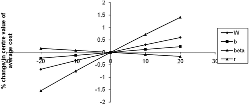
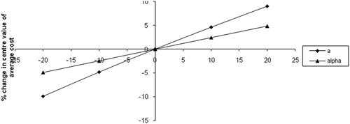
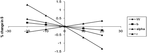
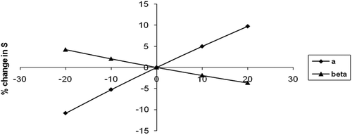
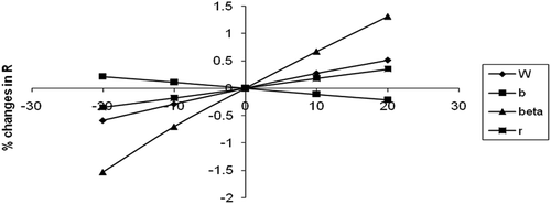
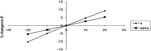
Using the given numerical example mentioned earlier, sensitivity analyses have been performed graphically for SFI policy with two different backlogging rates to study the effects of under- or overestimation of system parameters on the values of initial stock-level of stock-in period, maximum shortage level corresponding to the best found value of the average cost of the system (which is basically the minimum value of the average cost, but the property of minimization cannot be established theoretically). Here the percentage changes are taken as measures of sensitivity. These analyses have been carried out by changing (increasing and decreasing) the parameters by – 20% to + 20%. The results are obtained by changing one parameter at a time and keeping the other parameters at their original values. Considering the backlogging rate $\theta (t_s-t)=\frac{1}{1+\delta (t_s-t)}$, the results of these analyses are shown in Figures 2–7. It is to be noted that these computational works have been performed using the PSO-CO method.

Figure 2. Percentage changes in centre value of average cost w.r.t W, b,$\beta$ and r.

Figure 3. Percentage changes in centre value of average cost w.r.t a and $\alpha$.

Figure 4. Percentage changes in S w.r.t W, b, $\alpha$and r.

Figure 5. Percentage changes in S w.r.t a and $\beta$.

Figure 6. Percentage changes in R w.r.t W, b, $\beta$ and r.

Figure 7. Percentage changes in R w.r.t a and $\alpha$.

From the graphical sensitivity analysis (cf.Figures 2–7), the following observations can be made:

1. For both backlogging rates, the centre value of the average cost of the system is moderately sensitive with respect to the parameters a (the location parameter) and α (deterioration rate in OW). On the other hand, it is insensitive with the changes of W, b, $\beta$ and r.

2. It is also clear that the values of S and R are moderately sensitive with respect to a and α, whereas these are very less sensitive with respect to W, b, $\beta$ and r.

3. From Figure 4, it is observed that the value of S is less sensitive with the changes of W, b, α and r. However, in case of W, b and r, the changes are reverse.

7. Concluding remark

In inventory management, there arise two fundamental questions: when and where to stock the goods? Irrespective of where to reduce the system cost or to increase the profit, the management authorities are bound to replenish more goods (larger than the capacity of OW). The reason(s) behind this is/are to get the discount for bulk purchase or to reduce the costs of reordering, or to meet the higher demand, to avail the seasonal products with lower cost, etc. As a result, an additional storage space (termed as RW) is required to store the excess goods.

In this work, two other questions may arise:

1. Whether the optimization problems of different inventory policies can be solved using standard non-linear programming (NLP) technique or not?

2. How can one estimate the interval values of different parameters?

As the objective function of each optimization problem is interval valued, the existing NLP technique cannot be applied to solve the said problems. As a result, for solving the problems, different versions of PSO, interval mathematics and interval order relations have been applied. Basically, PSO is a very efficient soft computing technique used for computational optimization. In this optimization, the best found value of the objective function can be evaluated. In most of the cases, this value is either the global optimal value or very close to the optimal value. However, the optimality cannot be proved theoretically, although the convergence of the PSO technique has been established.

Regarding the estimation of interval valued parameters, one can easily estimate the values from the past experience.

In this paper, we have developed two inventory models with interval valued inventory costs with IFS as well as SFI policies and solved them with the help of PSO and interval order relations proposed by Sahoo et al. [30]. In each of the iterations of PSO-CO, interval order relations are used to find the best solution. From the computational results, it can be concluded that one can choose the model with SFI policy as it is less expensive to operate than the model with IFS policy.

For further study, one can extend the proposed models by incorporating some more realistic features, such as inventory-level-dependent demand, quantity discount, variable lead-time and interval valued demand.

Acknowledgements

The authors are grateful for valuable comments and suggestions from the respected reviewers. Their valuable comments and suggestions have enhanced the strength and significance of our paper.

Disclosure statement

No potential conflict of interest was reported by the authors.

Appendix A

In IFS policy, the inventory cycle starts with an instant order and ends with shortages. At the beginning (i.e., at time t = 0), the enterprise receives (S+R) units of a single product from the supplier. Then after fulfilling partially backlogged demand, the on-hand inventory level is S units. Out of these S units, W units are kept in OW and the remaining (S-W) units are stored in RW. The inventory level (S-W) units in RW are depleted gradually in the interval $0\le t\le t_r$ to meet the customers demand and deterioration effect of an item and it reaches zero at $t=t_r$. In OW, the inventory level W decreases during the interval $0\le t\le t_r$ due to deterioration only and during $t_r\le t\le t_o$ due to both demand and deterioration. At time $t=t_o$, the inventory level in OW reaches zero. Thereafter, shortages are allowed to occur during the time interval $t_o<t\le t_s$ with a rate $\theta (t_s-t)$. At time $t=t_s$(= T), the maximum shortage level is R. This entire cycle repeats after the end of the cycle length $t_s(=T)$ with the changed demand as it is time dependent. Our objective is to determine the optimal values of $t_r,t_o$ and $t_s$ in such a manner that the average cost of the system is minimized and also to obtain the corresponding values of S and R. The pictorial representation of the inventory situation is depicted in Figure A.1.

Figure A.1. Pictorial representation of two-warehouse inventory system with IFS policy.

During $0\le t\le t_r$, the inventory level decreases mainly to meet the demand by the customers and partly due to deterioration effect of the item, which are disposed continuously as they come to the selling point. Hence the rate of decrease of inventory level is equal to the deterioration of units and demand per unit time. As the rate of decrease of inventory level is denoted by $\frac{d{I}_r\left(t\right)}{dt}$, the corresponding differential equation can be written as follows:

(A.1) $\frac{d{I}_r\left(t\right)}{dt}+\beta I_r\left(t\right)=-f\left(t\right),0\le t\le t_r$(A.1)

with the condition

(A.2) $I_r\left(t\right)=0\mathrm{a}\mathrm{t}t=t_r.$(A.2)

(A.3) $Again,I_r\left(t\right)=S-W\mathrm{a}\mathrm{t}t=0.$(A.3)

Using (A.2), the solution of differential Equation (A.1) is given by

(A.4) $I_r\left(t\right)=exp\left(-\beta t\right)\underset{t}{\overset{t_r}{\int }}exp\left(\beta t\right)f\left(t\right)dt,0\le t\le t_r$(A.4)

Again from (A.3) and (A.4), we have

(A.5) $S=W+\underset{0}{\overset{t_r}{\int }}exp\left(\beta t\right)f\left(t\right)dt$(A.5)

Similarly, like (A.1), the differential equations corresponding to the inventory level $I_o\left(t\right)$ at OW during the time interval $0\le t\le t_s$ can be written as follows:

(A.6) $\frac{d{I}_o\left(t\right)}{dt}+\alpha I_o\left(t\right)=0,0\le t\le t_r$(A.6)

(A.7) $\frac{d{I}_o\left(t\right)}{dt}+\alpha I_o\left(t\right)=-f\left(t\right),t_r<t\le t_o$(A.7)

(A.8) $\frac{d{I}_o\left(t\right)}{dt}=-\theta \left(t_s-t\right)f\left(t\right),t_o<t\le t_s\left(=T\right)$(A.8)

subject to the conditions

(A.9) $I_o\left(t\right)=W\mathrm{a}\mathrm{t}t=0,$(A.9)

(A.10) $I_o\left(t\right)=0\mathrm{a}\mathrm{t}t=t_o$(A.10)

and $I_o\left(t\right)=-R\mathrm{a}\mathrm{t}t=t_s$(=T).(A.11)

Again, $I_o\left(t\right)$ is continuous at $t=t_r$ and $t_o$.

Using the conditions (A.9)–(A.11), the solutions of the differential Equations (A.6)–(A.8) are given by

(A.12) $I_o\left(t\right)=Wexp\left(-\alpha t\right),0\le t\le t_r$(A.12)

(A.13) $=exp\left(-\alpha t\right)\underset{t}{\overset{t_o}{\int }}exp\left(\alpha t\right)f\left(t\right)dt,t_r<t\le t_o$(A.13)

(A.14) $=R+\underset{t}{\overset{t_s}{\int }}\theta \left(t_s-t\right)f\left(t\right)dt{t}_o<t\le t_s\left(=T\right)$(A.14)

Using the continuity of $I_o\left(t\right)$ at time $t=t_r$ and $t=t_o$, we have

(A.15) $W=\underset{t_r}{\overset{t_o}{\int }}exp\left(\alpha t\right)f\left(t\right)dt$(A.15)

From which $t_r$ can be expressed in terms of $t_o$ and

(A.16) $R=-\underset{t_o}{\overset{t_s}{\int }}\theta \left(t_s-t\right)f\left(t\right)dt$(A.16)

Now the cumulative inventories in RW during $0\le t\le t_r$ and in OW during $0\le t\le t_o$ are $\underset{0}{\overset{t_r}{\int }}{I}_r\left(t\right)dt\mathrm{a}\mathrm{n}\mathrm{d}\underset{0}{\overset{t_o}{\int }}{I}_o\left(t\right)dt,$ respectively.

The present value of the inventory holding costs in RW and OW are $C_{hr}\underset{0}{\overset{t_r}{\int }}{e}^{-rt}{I}_r\left(t\right)dt$ and $C_{ho}\underset{0}{\overset{t_o}{\int }}{e}^{-rt}{I}_o\left(t\right)dt,$ respectively.

On the other hand, the present value of the backlogging and the opportunity cost due to lost sales are $C_b\underset{t_o}{\overset{t_s}{\int }}{e}^{-rt}\left[R+\underset{t}{\overset{t_s}{\int }}\theta \left(t_s-u\right)f\left(u\right)du\right]dt$ and $C_{ls}{e}^{-r{t}_s}\underset{t_o}{\overset{t_s}{\int }}\left[1-\theta \left(t_s-t\right)\right]f\left(t\right)dt,$ respectively.

Now the amounts of deteriorated units in both RW and OW during $0\le t\le t_o$ are $\beta \underset{0}{\overset{t_r}{\int }}{I}_r\left(t\right)dt\mathrm{a}\mathrm{n}\mathrm{d}\alpha \underset{0}{\overset{t_o}{\int }}{I}_o\left(t\right)dt,$ respectively.

The present value of the cost for deteriorated units is

(A.17) $C_p\left[\beta \underset{0}{\overset{t_r}{\int }}{e}^{-rt}{I}_r\left(t\right)dt+\alpha \underset{0}{\overset{t_o}{\int }}{e}^{-rt}{I}_o\left(t\right)dt\right].$(A.17)

Again, the present value of the shortage cost for the system is given by

(A.18) $C_{sho}=C_b\underset{t_o}{\overset{t_s}{\int }}{e}^{-rt}\left[R+\underset{t}{\overset{t_s}{\int }}\theta \left(t_s-u\right)f\left(u\right)du\right]dt$(A.18)

Here the cost function $TC{2}^{(1)}$ is an interval valued function of the variables $t_o$ and $t_s$. Let us suppose that $TC{2}^{(1)}\left(t_o,t_s\right)=\left[Z_L,Z_R\right]$, where

(A.19) $\begin{array}{l}{Z}^{\text{'}}{ }_L=[C_{oL}+C_{hrL}{\displaystyle \underset{0}{\overset{t_r}{\int }}{e}^{-rt}}{I}_r\left(t\right)dt+C_{hoL}{\displaystyle \underset{0}{\overset{t_o}{\int }}{e}^{-rt}}{I}_o\left(t\right)dt+C_{bL}{\displaystyle \underset{to}{\overset{t_s}{\int }}{e}^{-rt}}\left\{R+{\displaystyle \underset{t}{\overset{t_s}{\int }}\theta }\left(t_s-u\right)f\left(u\right)du\right\}dt\\ +C_{lsL}{e}^{-r{t}_s}{\displaystyle \underset{t_o}{\overset{t_s}{\int }}\left\{1-\theta \left(t_s-t\right)\right\}f\left(t\right)dt}+C_{pL}\left\{\beta {\displaystyle \underset{0}{\overset{t_r}{\int }}{e}^{-rt}}{I}_r\left(t\right)dt+\alpha {\displaystyle \underset{0}{\overset{t_o}{\int }}{e}^{-rt}}{I}_o\left(t\right)dt\right\}]/T\end{array}$(A.19)

and

(A.20) $\begin{array}{l}{Z}_R=[C_{oR}+C_{hrR}{\displaystyle \underset{0}{\overset{t_r}{\int }}{e}^{-rt}}{I}_r\left(t\right)dt+C_{hoR}{\displaystyle \underset{0}{\overset{t_o}{\int }}{e}^{-rt}}{I}_o\left(t\right)dt+C_{bR}{\displaystyle \underset{to}{\overset{t_s}{\int }}{e}^{-rt}}\left\{R+{\displaystyle \underset{t}{\overset{t_s}{\int }}\theta }\left(t_s-u\right)f\left(u\right)du\right\}dt\\ +C_{lsR}{e}^{-r{t}_s}{\displaystyle \underset{t_o}{\overset{t_s}{\int }}\left\{1-\theta \left(t_s-t\right)\right\}f\left(t\right)dt}+C_{pR}\left\{\beta {\displaystyle \underset{0}{\overset{t_r}{\int }}{e}^{-rt}}{I}_r\left(t\right)dt+\alpha {\displaystyle \underset{0}{\overset{t_o}{\int }}{e}^{-rt}}{I}_o\left(t\right)dt\right\}]/T\end{array}$(A.20)

Hence our problem is as follows:

(A.21) $\begin{array}{rl}& \mathrm{M}\mathrm{i}\mathrm{n}\mathrm{i}\mathrm{m}\mathrm{i}\mathrm{z}\mathrm{e}TC{2}^{(1)}\left(t_o,t_s\right)\\ & \mathrm{s}\mathrm{u}\mathrm{b}\mathrm{j}\mathrm{e}\mathrm{c}\mathrm{t}\mathrm{t}\mathrm{o}{t}_s>t_{o}and{t}_o>0\end{array}$(A.21)

This is a non-linear minimization problem with interval objective.

Now we have to solve the non-linear minimization problem (A.21) with interval valued objective. For solving this problem, we have developed an efficient soft computing method, viz. PSO.

References

- V.R. Hartely, Operations Research: A Managerial Emphasis, Good Year, Santa Monica, CA, 1976, pp. 315–317. ( Chapter 12).
- B. Das, K. Maity, and M. Maiti, A two warehouse supply chain model under possibility/necessity/credibility measures, Math. Comp. Model. 46 (2007), pp. 398–409. doi:10.1016/j.mcm.2006.11.017
- B. Niu and J. Xie, A note on two-warehouse inventory model with deterioration under FIFO dispatch policy, Eur. J. Oper. Res. 190 (2008), pp. 571–577. doi:10.1016/j.ejor.2007.06.027
- M. Rong, N.K. Mahapatra, and M. Maiti, A two warehouse inventory model for a deteriorating item with partially/fully backlogged shortage and fuzzy lead time, Eur. J. Oper. Res. 189 (2008), pp. 59–75. doi:10.1016/j.ejor.2007.05.017
- C.K. Jaggi, A. Khanna, and P. Verma, Two-warehouse partial backlogging inventory model for deteriorating items with linear trend in demand under inflationary conditions, Int. J. Syst. Sci. 42 (2011), pp. 1185–1196. doi:10.1080/00207720903353674
- P.M. Ghare and G.F. Shrader, A model for exponentially decaying inventories, J. Ind. Eng. 14 (1963), pp. 238–243.
- R.P. Covert and G.C. Philip, An EOQ model for items with weibull distribution deterioration, Am. Inst. Ind. Eng. Trans. 5 (1973), pp. 323–326.
- Y.K. Shah, An order-level lot-size inventory for deteriorating items, Am. Inst. Ind. Eng. Trans. 9 (1977), pp. 108–112.
- R.S. Sachan, On (T,Si) policy inventory model for deteriorating items with time proportion demand, J. Oper. Res. Soc. 35 (1984), pp. 1013–1019.
- S. Kang and I. Kim, A study on the price and production level of the deteriorating inventory system, Int. J. Production Res. 21 (1983), pp. 899–908. doi:10.1080/00207548308942422
- A.K. Bhunia and A.A. Shaikh, A two warehouse inventory model for deteriorating items with time dependent partial backlogging and variable demand dependent on marketing strategy and time, Int. J. Inventory Control Manag. 1 (2011a), pp. 95–110.
- A.K. Bhunia and A.A. Shaikh, A deterministic model for deteriorating items with displayed inventory level dependent demandrate incorporating marketing decisions with transportation cost, Int. J. Ind. Eng. Computations 2 (2011b), pp. 547–562. doi:10.5267/j.ijiec.2011.03.004
- A.K. Bhunia, A.A. Shaikh, A.K. Maiti, and M. Maiti, A two warehouse deterministic inventory model for deteriorating items with a linear trend in time dependent demand over finite time horizon by Elitist Real-Coded Genetic Algorithm, Int. J. Ind. Eng. Computations 4 (2013), pp. 241–258. doi:10.5267/j.ijiec
- A.K. Bhunia and A.A. Shaikh, A deterministic inventory model for deteriorating items with selling price dependent demand and three-parameter weibull distributed deterioration, Int. J. Ind. Eng. Computations 5 (2014), pp. 495–510. doi:10.5267/j.ijiec.2014.2.002
- K.J. Chung, L.E.C. Barron, and P.S. Ting, An inventory model with non-instantaneous receipt and exponentially deteriorating items for an integrated three layer supply chain system under two levels of trade credit, Int. J. Production Econ. 155 (2014), pp. 310–317. doi:10.1016/j.ijpe.2013.12.033
- J. Wu, L.-Y. Ouyang, L.E.C. Cárdenas-Barrón, and S.K. Goyal, Optimal credit period and lot size for deteriorating items with expiration dates under two-level trade credit financing, Eur. J. Oper. Res. 237 (2014), pp. 898–908. doi:10.1016/j.ejor.2014.03.009
- J.A. Buzacott, Economic order quantities with inflation, Oper. Res. Q. 26 (1975), pp. 553–558. doi:10.1057/jors.1975.113
- H. Bierman and J. Thomas, Inventory decisions under inflationary conditions, Decis. Sci. 8 (1977), pp. 151–155. doi:10.1111/deci.1977.8.issue-1
- P. Vrat and G. Padmanabhan, An inventory model under inflation for stock dependent consumption rate items, Eng. Costs Production Econ. 19 (1990), pp. 379–383. doi:10.1016/0167-188X(90)90068-S
- T.K. Datta and A.K. Pal, Effects of inflation and time-value of money on an inventory model with linear time-dependent demand rate and shortages, Eur. J. Oper. Res. 52 (1991), pp. 326–333. doi:10.1016/0377-2217(91)90167-T
- H.-M. Wee and S.-T. Law, Replenishment and pricing policy for deteriorating items taking into account the time-value of money, Int. J. Production Econ. 71 (2001), pp. 213–220. doi:10.1016/S0925-5273(00)00121-3
- H.-L. Yang, J.-T. Teng, and M.-S. Chern, Deterministic inventory lot-size models under inflation with shortages and deterioration for fluctuating demand, Nav. Res. Log. 48 (2001), pp. 144–158. doi:10.1002/(ISSN)1520-6750
- C.K. Jaggi, K.K. Aggarwal, and S.K. Goel, Optimal order policy for deteriorating items with inflation induced demand, Int. J. Production Econ. 34 (2006), pp. 151–155. doi:10.1016/0925-5273(94)90031-0
- T.-P. Hsieh, C.-Y. Dye, and L.-Y. Ouyang, Determining optimal lot size for a two-warehouse system with deterioration and shortages using net present value, Eur. J. Oper. Res. 191 (2008), pp. 182–192. doi:10.1016/j.ejor.2007.08.020
- J.K. Dey, S.K. Mondal, and M. Maiti, Two storage inventory problem with dynamic demand and interval valued lead-time over finite time horizon under inflation and time-value of money, Eur. J. Oper. Res. 185 (2008), pp. 170–194. doi:10.1016/j.ejor.2006.12.037
- H.-L. Yang, Two-warehouse inventory models for deteriorating items with shortages under inflation, Eur. J. Oper. Res. 157 (2004), pp. 344–356. doi:10.1016/S0377-2217(03)00221-2
- H.-L. Yang, Two-warehouse partial backlogging inventory models for deteriorating items under inflation, Int. J. Production Econ. 103 (2006), pp. 362–370. doi:10.1016/j.ijpe.2005.09.003
- R.E. Moore, Methods and Applications of Interval Analysis, SIAM, Philadelphia, 1979.
- S. Karmakar, S.K. Mahato, and A.K. Bhunia, Interval oriented multi-section techniques for global optimization, J. Comput. Appl. Math. 224 (2009), pp. 476–491. doi:10.1016/j.cam.2008.05.025
- L. Sahoo, A.K. Bhunia, and P.K. Kapur, Genetic algorithm based multi-objective reliability optimization in interval environment, Computers Ind. Eng. 62 (2012), pp. 152–160. doi:10.1016/j.cie.2011.09.003
- R.C. Eberhart and J.F. Kennedy, A new optimizer using particle swarm theory, Proceedings of the Sixth International Symposium on Micro Machine and Human Science, Municipal Industrial Research Institute, Nagoya, October 4–6, 1995, pp. 39–43.
- J.F. Kennedy and R.C. Eberhart, Particle swarm optimization, Proceedings of the IEEE International Conference on Neural Network, Vol. IV, Perth, November 27–December 1, 1995, pp. 1942–1948. IEEE Press.
- M. Clerc, The swarm and queen: towards a deterministic and adaptive particle swarm optimization, Proceedings of 1999 IEEE Congress on Evolutionary Computation, Washington, DC, July 6–9, 1999, pp. 1951–1957.
- M. Clerc and J.F. Kennedy, The particle swarm - explosion, stability, and convergence in a multidimensional complex space, IEEE Transection Evol. Comput. 6 (2002), pp. 58–73. doi:10.1109/4235.985692
- J. Sun, B. Feng, and W.B. Xu, Particle swarm optimization with particles having quantum behavior, IEEE Proceedings of Congress on Evolutionary Computation, CEC 2004, Portland, OR, June 19–23, 2004, pp. 325–331.
- J. Sun, W.B. Xu, and B. Feng, A global search strategy of quantum-behaved particle swarm optimization, Proceedings of the 2004 IEEE Conference on Cybernetics and Intelligent Systems, CIS, Singapore, December 1–3, 2004, pp. 111–116.
- D. Pan, Y. Ci, M. He, and H. He, An improved quantum-behaved particle swarm optimization algorithm based on random weight, J. Software 8 (2013), pp. 1327–1332. doi:10.4304/jsw.8.6.1327-1332
- M. Xi, J. Sun, and W. Xu, An improved quantum-behaved particle swarm optimization algorithm with weighted mean best position, Appl. Math. Comput. 205 (2008), pp. 751–759. doi:10.1016/j.amc.2008.05.135
- J. Sun, W.B. Xu, and B. Feng, Adaptive parameter selection of quantum-behaved particle swarm optimization on global level, Adv. Intell. Computing, Lecture Notes Comput. Sci. 3644 (2005), pp. 420–428.
- L.S. Coelho, Gaussian quantum-behaved particle swarm optimization approachesfor constrained engineering design problems, Expert Syst. Appl. 37 (2010), pp. 1676–1683. doi:10.1016/j.eswa.2009.06.044
- A.K. Bhunia, A.A. Shaikh, and R.K. Gupta, A study on two-warehouse partially backlogged deteriorating inventory models under inflation via particle swarm optimisation, Int. J. Syst. Sci. 46 (2015), pp. 1036–1050. doi:10.1080/00207721.2013.807385