Multiscale modelling of solute transport through porous media using homogenization and splitting methods

ABSTRACT

The aim of this paper is to treat multiscale modelling approaches for solute transport through porous media. This involves coupled systems of convection–diffusion–reaction equations that can be homogenized and solved by splitting methods. The topic is very challenging in the case of multiscale model systems, for example, those arising when the evolution of several chemical species involves time-dependent or non-linear mechanisms. Our proposed modelling approach is based on the idea of homogenization of the diffusion, convection and reaction of chemical species in a porous medium to derive macroscopic equations. Based on the existence of multiple timescales, we introduce multiscale methods to model the evolution and obtain solutions. A more detailed analysis shows that such multiscale methods can be treated via the so-called iterative splitting approach. To solve the multiscale model, we propose exact solutions of some submodels, which can be then be taken into account and play an important role in accelerating the numerical computations of the large coupled model. In the first part, we introduce the model and its application. In the second part, we discuss the analytical solutions of the submodels related to fast and analytically solvable convection–reaction equations. The iterative splitting approaches are then discussed for solving the multiple timescale part. Finally, the last part presents some numerical experiments involving real-life test problems in transport–reaction processes.

KEYWORDS:

• Multiscale modelling approach
• solute transport through porous media
• homogenization
• convection–diffusion–reaction equations
• splitting methods
• mobile–immobile transport
• analytical solutions
• iterative splitting approach

1. Introduction

The motivation is to derive macroscopic time-dependent models for fluid transport problems, for example, deposition processes based on chemical vapour problems [1], groundwater reservoir processes [2, 3], chemical reactors [4], and climate models [5], which are based on microscopic models in porous media.

Such models have multiple scales, both spatial and temporal, and we apply homogenization methods and also multiple timescale methods to derive a macroscopic model comprising coupled transport–reaction–equations with mobile and immobile areas, see [6].

Based on the different spatial and temporal scales for each part of the system of equations, it is important to discuss the modelling with multiple scales of their behaviour, see the ideas in [7–10].

Such multiscale modelling approaches allow decomposing the model into simpler submodels, which can then be solved without neglecting the behaviour of the full model, see [10]. Here, we will derive macroscopic models which are based on microscopic models after being homogenized in space, and then treated according to multiple timescale modelling approaches to obtain hierarchical submodels with different temporal scales, see [11].

The new contribution of this paper, in contrast to the previous papers [12,13], is that we start with the microscopic models, which are based on multiple scales, and derive an upscaled macroscopic model with different scales and then formulate a hierarchical system of equations, see [14].

To treat this system of hierarchical equations, we will begin by considering how the appropriate methods and underlying numerical analysis should be selected to deal with such model equations.

We have proved that perturbation methods, both linear and non-linear, can be considered as a modified iterative splitting approach, see [14]. Such methods are quick and highly accurate.

Numerically, we can solve such models with so-called iterative splitting approaches that allow decomposing them into simpler subproblems, see [12,15]. Here the underlying solver idea is to embed some semi-analytical solutions of the simpler subproblems and implement them inside a multiscale splitting approach. We extend the analytical solutions to space- and time-dependent velocity and diffusion coefficients for one-dimensional (1D) problems. Such solutions can be embedded as a priori test functions into two-dimensional (2D)and three-dimensional (3D) problems, see [16].

Figure 1 presents this multiscale modelling approach starting from a microscopic model.

Figure 1. Multiscale modelling in time and space of a porous media model.

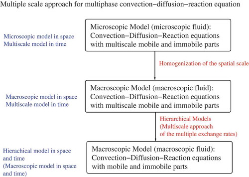
Here our contribution is to derive the upscaled macroscopic model and apply the splitting approach to solve the spatial and time-dependent coupled transport and reaction models with simpler submodels. Further, we present multiphase problems based on the simulation of a 1D problem related to transport problems through porous media.

This paper is organized as follows. The mathematical model is described in Section 2. The splitting methods, which solve the simpler model equations, which are time-dependent convection–reaction equations, are described in Section 3. The verification of the new discretization method for the multiscale modelling approach is given in various numerical examples and is carried out in Section 4. At the end of this paper, future lines of work will be outlined.

2. Mathematical model

Modelling gaseous transport in fluid transport problems, for example, solute transport problems or plasma reactors, gives us a multiscale problem. One can concentrate on two modelling directions:

• Spatial multiscales: Upscaling of the porous medium (homogenization theory), see [1].

• Temporal multiscales: Hierarchical equations based on the multiple timescales (perturbation theory), see [17].

Our model is based on the assumption that we have m chemical species, which are dissolved in a fluid (gaseous or liquid phase), see [1,2].

In the following, we deal with two multiscale methods to address adequately the multiple temporal and spatial scales:

• Homogenization of the spatial variables (upscaling of the microscopic space);

• Multiple timescales of the temporal variable (hierarchical equations for the different timescales).

In the following, we present the different methods with the underlying models.

2.1. Microscopic model and homogenization of the spatial variables

We deal with a porous medium $\mathrm{\Omega },$ for example, for simplicity, taken as a unit cube with $\mathrm{\Omega }$ with $n=2,3$ and we make the following definitions, see also [18]:

Definition 2.1:

We define the union of the pore spaces as:

(1) ${\mathrm{\Omega }}_f^{\in }=\mathrm{\Omega }\cap {\cup }_{k\in {\mathbb{Z}}^n}\in (Y_f+k),$(1)

where $Y\in ]0,1{[}^n,n=2,3$ is the unit cell and the boundary is given as $\mathrm{\partial }\mathrm{\Omega }={\bar{\mathrm{\Gamma }}}^1\cup {\bar{\mathrm{\Gamma }}}^2$ with ${\mathrm{\Gamma }}^1\cap {\mathrm{\Gamma }}^2=0$ and each boundary ${\mathrm{\Gamma }}^1,{\mathrm{\Gamma }}^2$ is an $n-1$ dimensional manifold. Further, $\in >0$ is the parameter for constructing the microscopic scales of the porous media.

The geometry of the cell Y (porous media cells) is given in Definition 2.2.

Definition 2.2:

We have Y_m is a mobile pellet, and Y_im is an immobile pellet, each as a connected open subset of ${\mathbb{R}}^n$ with ${\bar{Y}}_m,{\bar{Y}}_{im}\subset Y,$ and we have Lipschitz boundaries.

Further, the inter-aggregate pore means the fluid area of the pore and is given as $Y_f=Y\mathrm{\setminus }({\bar{Y}}_m\cup {\bar{Y}}_{im}).$

Further, ${\mathrm{\Omega }}_m^{\in }$ is the union of all mobile pellets and ${\mathrm{\Gamma }}_m^{\in }$ is the boundary between ${\mathrm{\Omega }}_m^{\in }$ and ${\mathrm{\Omega }}_f^{\in },{\mathrm{\Omega }}_{im}^{\in }$ is the union of all immobile pellets and ${\mathrm{\Gamma }}_{im}^{\in }$ is the boundary between ${\mathrm{\Omega }}_{im}^{\in }$ and ${\mathrm{\Omega }}_f^{\in }.$

${\mathrm{\Gamma }}_{m,im}^{\in }$ is the boundary between ${\mathrm{\Omega }}_m^{\in }$ and ${\mathrm{\Omega }}_{im}^{\in }$ and ${\mathrm{\Gamma }}^{\in }={\mathrm{\Gamma }}_m^{\in }\cup {\mathrm{\Gamma }}_{im}^{\in }\cup {\mathrm{\Gamma }}_{m,im}^{\in }.$

Hence, our porous media is given as: $\mathrm{\Omega }={\mathrm{\Omega }}_m^{\in }\cup {\mathrm{\Omega }}_{im}^{\in }\cup {\mathrm{\Omega }}_f^{\in }\cup {\mathrm{\Gamma }}^{\in }.$

Definition 2.3:

For $q\in [1,\mathrm{\infty }],k\in \mathbb{N}$ and $\mathrm{\Omega }$ an open subset of ${\mathbb{R}}^d,$ let

(2) $W_{loc}^{k,q}(\mathrm{\Omega })=\left\{f\in L^p(\mathrm{\Omega }):{\mathrm{\partial }}^{\tilde{k}}f\in L_{loc}^p\left(\mathrm{\Omega }\right)(weakly)\mathrm{\forall }|\tilde{k}|\le k\right\},$(2)

(3) $W^{k,q}(\mathrm{\Omega })=\left\{f\in L^p(\mathrm{\Omega }):{\mathrm{\partial }}^{\tilde{k}}f\in L^p\left(\mathrm{\Omega }\right)(weakly)\mathrm{\forall }|\tilde{k}|\le k\right\},$(3)

where the multi-index $\tilde{k}$ with $|\tilde{k}|={\tilde{k}}_1+\dots +{\tilde{k}}_n<\le k$ and we have the spatial derivative $\frac{{\mathrm{\partial }}^{{\tilde{k}}_1}}{{{\mathrm{\partial }}_{x_1}}^{{\tilde{k}}_1}}\dots \frac{{\mathrm{\partial }}^{{\tilde{k}}_n}}{{{\mathrm{\partial }}_{x_n}}^{{\tilde{k}}_n}}u.$ The Banach space is given as $L^p\left(\mathrm{\Omega }\right)$ and the locally compact Banach space is $L_{loc}^p(\mathrm{\Omega }),$ see [19].

Definition 2.4:

The microscopic fluid pore space (mobile phase) is given as ${\mathrm{\Omega }}_f^{\in }$ while the microscopic solid space (immobile phase) is given as ${\mathrm{\Omega }}_{im}^{\in }$ and the microscopic pore space is $\mathrm{\Omega }={\mathrm{\Omega }}_f^{\in }\cup {\mathrm{\Omega }}_m^{\in }\cup {\mathrm{\Omega }}_{im}^{\in }\cup {\mathrm{\Gamma }}^{\in }.$

Further, we assume the homogenization results of [18,20], which allow upscaling the microscopic space to a macroscopic space, which means that there exists a continuous linear operator ${\mathrm{\Pi }}_{\in }:W^{1,q}\left({\mathrm{\Omega }}_f^{\in }\right)\to W_{loc}^{1,q}(\mathrm{\Omega })$ and we have $\mathrm{\forall }u\in W^{1,q}\left({\mathrm{\Omega }}_f^{\in }\right)$ and constants $k_1,k_2,k_3>0:$

(4) ${\mathrm{\Pi }}_{\in }u=u,\mathrm{i}\mathrm{n}{\mathrm{\Omega }}_f^{\in },$(4)

(5) ${\int }_{\mathrm{\Omega }(\in k_0)}{\left|{\mathrm{\Pi }}_{\in }u\right|}^{q}dx\le k_1(Y_f,n,q){\int }_{{\mathrm{\Omega }}_f^{\in }}{\left|u\right|}^{q}dx,$(5)

(6) ${\int }_{\mathrm{\Omega }(\in k_0)}{\left|\mathrm{\nabla }{\mathrm{\Pi }}_{\in }u\right|}^{q}dx\le k_2(Y_f,n,q){\int }_{{\mathrm{\Omega }}_f^{\in }}{\left|\mathrm{\nabla }u\right|}^{q}dx,$(6)

where $\mathrm{\Omega }(\in k_0)\left\{x\in \mathrm{\Omega }:dist(x,\mathrm{\partial }\mathrm{\Omega })>\in k_0\right\}.$

In the first step, we homogenize with respect to the porous medium, which means the spatial variable. We deal with the following microscopic equation in one component:

(7) ${\mathrm{\partial }}_t{u}^{\in }+\mathrm{\nabla }\cdot {\mathbf{v}}^{\in }(x,t)u^{\in }-\mathrm{\nabla }D(x,t)\mathrm{\nabla }{u}^{\in }=f(u^{\in }),\mathrm{i}\mathrm{n}{\mathrm{\Omega }}_f^{\in }\times (0,T),$(7)

(8) ${\mathrm{\partial }}_t{g}^{\in }+{\in }^2(\mathrm{\nabla }\cdot {\mathbf{v}}^{\in }(x,t)g^{\in }-\mathrm{\nabla }D(x,t)\mathrm{\nabla }{g}^{\in }=f(g^{\in }),\mathrm{i}\mathrm{n}{\mathrm{\Omega }}_{im}^{\in }\times (0,T),$(8)

(9) $({\mathbf{v}}^{\in }{u}^{\in }-D\mathrm{\nabla }{u}^{\in })\cdot \vec{n}={\in }^2({\mathbf{v}}^{\in }{g}^{\in }-D\mathrm{\nabla }{g}^{\in })\cdot \vec{n},\mathrm{o}\mathrm{n}{\mathrm{\Gamma }}_{f,im}^{\in }\times (0,T),$(9)

where ${\mathrm{\Gamma }}_{f,im}^{\in }={\mathrm{\Omega }}_f^{\in }\cap {\mathrm{\Omega }}_{im}^{\in }.$ The unknown mobile concentrations are $u^{\in }=u^{\in }(x,t)$ and the unknown immobile concentrations are $g^{\in }=g^{\in }(x,t).$ The reaction part is given by a non-linear function $f:W^{1,q}({\mathrm{\Omega }}^{\in })\to W^{1,q}({\mathrm{\Omega }}^{\in }).\mathbf{v}$ is the space- and time-dependent velocity and D is the space- and time-dependent diffusion in the microscopic space.

Assumption 2.5:

For the immobile phase, we assume that we have such small scales in space, that we could skip the space-dependent operators. This means that the diffusion and convection term are neglected, see also [2].

Further, we have the microscopic scale $y=\frac{x}{\in }$ and $x\in {\mathbb{R}}^{2,3}$ is the macroscopic scale and we average over the microscopic scale, which constitutes a process of upscaling, and rewrite this to get

(10) $\begin{array}{rl}\rho {\mathrm{\partial }}_t{\bar{u}}^{\in }+\rho {\mathrm{\nabla }}_x\cdot {\bar{\mathrm{v}}}^{\in }{\bar{u}}^{\in }-\rho {\mathrm{\nabla }}_x\bar{D}{\mathrm{\nabla }}_x{\bar{u}}^{\in }=& \rho f({\bar{u}}^{\in })-\beta b({\bar{u}}^{\in },{\bar{g}}^{\in }),\mathrm{i}\mathrm{n}{\mathrm{\Omega }}^{\in }\times (0,T),\\ {\rho }_{im}{\mathrm{\partial }}_t{\bar{g}}^{\in }=& {\rho }_{im}f({\bar{g}}^{\in })+\beta b({\bar{u}}^{\in },{\bar{g}}^{\in }),\mathrm{i}\mathrm{n}{\mathrm{\Omega }}^{\in }\times (0,T),\end{array}$(10)

where $\rho ,{\rho }_{im}$ are the mobile and immobile porosity with $\rho +{\rho }_{im}=1$ and for a standard mobile–immobile rate, see [2,21], we have $\beta b({\bar{u}}^{\in },{\bar{g}}^{\in })=\beta ({\bar{u}}^{\in }-{\bar{g}}^{\in }),$ where $\beta$ is the exchange rate.

Further, we have the convergence of the continuous operator, which means: ${\bar{u}}^{\in },{\bar{g}}^{\in }\to (u,g)$ and the upscaled macroscopic equation is obtained.

Proposition 2.6:

Suppose given the microscopic system of Equations (7)–(9) based on the porous medium given in Definition 2.4.

We apply the homogenization in the spatial variables with respect to the porous cell and obtain, after the convergence of the averaged variables, the following system of upscaled macroscopic equations:

(11) $\rho {\mathrm{\partial }}_{t}u+{\mathrm{\nabla }}_x\cdot \mathrm{v}(x,t)u-{\mathrm{\nabla }}_{x}D(x,t){\mathrm{\nabla }}_{x}u=\rho f(c)-\beta b(c,g),in\mathrm{\Omega }\times (0,T),$(11)

(12) ${\rho }_{im}{\mathrm{\partial }}_{t}g={\rho }_{im}f(g)+\beta b(u,g),in\mathrm{\Omega }\times (0,T).$(12)

The proof is as follows.

Proof.

Based on the microscale variable $y=\frac{x}{\in },$ the derivatives are

(13) $\mathrm{\nabla }={\mathrm{\nabla }}_x+\frac{1}{\in }{\mathrm{\nabla }}_y,$(13)

we put these into Equations (7)–(9) and have

(14) $\begin{array}{rl}& {\mathrm{\partial }}_t{u}^{\in }+{\mathrm{\nabla }}_x\cdot {\mathbf{v}}^{\in }{u}^{\in }-{\mathrm{\nabla }}_x\cdot D{\mathrm{\nabla }}_x{u}^{\in }\\ & +\frac{1}{\in }{\mathrm{\nabla }}_y\cdot \left({\mathbf{v}}^{\in }{u}^{\in }-D({\mathrm{\nabla }}_x+\frac{1}{\in }{\mathrm{\nabla }}_y)u^{\in }\right)=f(c^{\in }),\mathrm{i}\mathrm{n}{\mathrm{\Omega }}_f^{\in }\times (0,T),\end{array}$(14)

(15) $\begin{array}{rl}& {\mathrm{\partial }}_t{g}^{\in }+{\in }^2({\mathrm{\nabla }}_x\cdot {\mathbf{v}}^{\in }{g}^{\in }-{\mathrm{\nabla }}_x\cdot D{\mathrm{\nabla }}_x{g}^{\in })\\ & +{\in }^2\frac{1}{\in }{\mathrm{\nabla }}_y\cdot \left({\mathbf{v}}^{\in }{g}^{\in }-D({\mathrm{\nabla }}_x+\frac{1}{\in }{\mathrm{\nabla }}_y)g^{\in }\right)=f(g^{\in }),\mathrm{i}\mathrm{n}{\mathrm{\Omega }}_{im}^{\in }\times (0,T).\end{array}$(15)

We average over the microscopic domain ${\mathrm{\Omega }}_f^{\in }$ and ${\mathrm{\Omega }}_{im}^{\in }:$

(16) $\frac{1}{\left|{\mathrm{\Omega }}_f^{\in }\right|}{\int }_{{\mathrm{\Omega }}_f^{{\hspace{0.17em}}^{\in }}}{u}^{\in }dV={\bar{u}}^{\in },$(16)

(17) $\frac{1}{\left|{\mathrm{\Omega }}_{im}^{\in }\right|}{\int }_{{\mathrm{\Omega }}_{im}^{{\hspace{0.17em}}^{\in }}}{g}^{\in }dV={\bar{g}}^{\in },$(17)

where $\left|{\mathrm{\Omega }}_f^{\in }\right|$ and $\left|{\mathrm{\Omega }}_{im}^{\in }\right|$ are the measures for the three-dimensional volume in the mobile and immobile domain.

Now, we apply Gauss’s Theorem at the boundary of the two phases:

(18) ${\int }_{{\mathrm{\Omega }}_f^{\in }}{\mathrm{\nabla }}_y\cdot ({\mathbf{v}}^{\in }{u}^{\in }-D({\mathrm{\nabla }}_x+\frac{1}{\in }{\mathrm{\nabla }}_y)u^{\in }dV$(18)

(19) $={\int }_{{\mathrm{\Gamma }}^{\in }}({\mathbf{v}}^{\in }{u}^{\in }-D({\mathrm{\nabla }}_x+\frac{1}{\in }{\mathrm{\nabla }}_y)u^{\in })\cdot \vec{n}d\mathrm{\Gamma }$(19)

(20) $={\int }_{{\mathrm{\Gamma }}^{\in }}\in b(u^{\in },g^{\in })d\mathrm{\Gamma }=\beta \frac{1}{\in }b(u^{\in },g^{\in }),$(20)

where we have used the assumption that the actual mobile–immobile rate (this is also possible for the adsorption rate) is given by

(21) $({\mathbf{v}}^{\in }{u}^{\in }-D({\mathrm{\nabla }}_x+\frac{1}{\in }{\mathrm{\nabla }}_y)u^{\in })\cdot \vec{n}=\in b(u^{\in },g^{\in }).$(21)

We apply the same idea to the immobile phase Equations (15), and obtain

(22) ${\int }_{{\mathrm{\Omega }}_{im}^{\in }}{\mathrm{\nabla }}_y\cdot ({\mathbf{v}}^{\in }{g}^{\in }-D({\mathrm{\nabla }}_x+\frac{1}{\in }{\mathrm{\nabla }}_y)g^{\in }dV$(22)

(23) $=-{\int }_{{\mathrm{\Gamma }}^{\in }}({\mathrm{v}}^{\in }{g}^{\in }-D({\mathrm{\nabla }}_x+\frac{1}{\in }{\mathrm{\nabla }}_y)g^{\in })\cdot \vec{n}d\mathrm{\Gamma }$(23)

(24) $=-{\int }_{{\mathrm{\Gamma }}^{\in }}\frac{1}{\in }b(u^{\in },g^{\in })\mathrm{\Gamma }=-\beta \frac{1}{\in }b(u^{\in },g^{\in }),$(24)

where we apply the relation $({\mathbf{v}}^{\in }{g}^{\in }-D({\mathrm{\nabla }}_x+\frac{1}{\in }{\mathrm{\nabla }}_y)g^{\in })\cdot \vec{n}=\frac{1}{{\in }^2}({\mathbf{v}}^{\in }{u}^{\in }-D({\mathrm{\nabla }}_x+\frac{1}{\in }{\mathrm{\nabla }}_y)u^{\in })\cdot \vec{n}$ and $b(u^{\in },g^{\in })$ is the actual mobile–immobile rate depending on $u^{\in },g^{\in }.$

Further, we obtain the averaged results:

(25) $\begin{array}{rl}& \rho {\mathrm{\partial }}_t{\bar{u}}^{\in }+\rho {\mathrm{\nabla }}_x\cdot {\bar{\mathrm{v}}}^{\in }{\bar{u}}^{\in }-\rho {\mathrm{\nabla }}_x\bar{D}{\mathrm{\nabla }}_x{\bar{u}}^{\in }=\rho f({\bar{c}}^{\in })-\beta b({\bar{c}}^{\in },{\bar{g}}^{\in }),\mathrm{i}\mathrm{n}{\mathrm{\Omega }}^{\in }\times (0,T),\\ & {\rho }_{im}{\mathrm{\partial }}_t{\bar{g}}^{\in }={\rho }_{im}f({\bar{g}}^{\in })+\beta b({\bar{c}}^{\in },{\bar{g}}^{\in }),\mathrm{i}\mathrm{n}{\mathrm{\Omega }}^{\in }\times (0,T).\end{array}$(25)

We apply the continuous linear operator ${\mathrm{\Pi }}_{\in },$ see also [18,20] for the adsorption phase, and obtain the results (11)–(12).

Remark 2.7:

The generalization to m species is straightforward, see [20].

2.2. Hierarchical model in space and time (full macroscopic model)

In the following, we deal with the spatially upscaled one-species model given in (11)–(12). Such models are used for migration of pollutants in a porous media. We assume we have an underlying geosphere, for example, underlying rock and soil of a waste disposal site, which has been polluted and we are interested in simulating the transport of the pollutants through the geosphere to the earth’s surface (biosphere), see [22,23].

2.2.1. Full macroscopic model

The models are based on an exchange between the mobile and immobile phase concentrations, which are presented in Figure 2.

Figure 2. Porous media model with mobile and immobile phases.

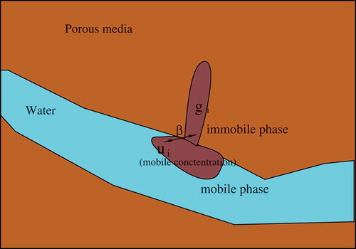
The system of such a waste disposal simulation is given in the generalization to m species (pollutant) in the following model equation, see [20]; here, we have also formulated the reaction part of the species:

(26) $\begin{array}{rl}& \rho {\mathrm{\partial }}_t{u}_i+\mathrm{\nabla }\cdot \mathbf{v}(x,t)u_i+\mathrm{\nabla }D(x,t)\cdot \mathrm{\nabla }{u}_i\\ & =\rho f_i(u_1,\dots ,u_m)+{\tilde{f}}_i(u_1,\dots ,u_m,g_1,\dots ,g_m)\mathrm{i}\mathrm{n}\mathrm{\Omega }\times (0,T),\end{array}$(26)

(27) $u_i(x,0)=u_i,0(x),\mathrm{o}\mathrm{n}\mathrm{\Omega },$(27)

(28) $u_i(x,t)={\tilde{u}}_i(x,t)\mathrm{o}\mathrm{n}\mathrm{\partial }\mathrm{\Omega }\times (0,T),$(28)

(29) ${\rho }_{im}{\mathrm{\partial }}_t{g}_i={\rho }_{im}{f}_i(g_1,\dots ,g_m)-{\tilde{f}}_i(u_1,\dots ,u_m,g_1,\dots ,g_m)\mathrm{i}\mathrm{n}\mathrm{\Omega }\times (0,T),$(29)

(30) $g_i(x,0)={g_{i,}}_0(x)\mathrm{o}\mathrm{n}\mathrm{\Omega },$(30)

$i=1,\dots ,m,$

where m is the number of equations and i is the index of each component. The unknown mobile concentrations $u_i=u_i(x,t)$ are taken in $\mathrm{\Omega }\times (0,T)\subset {\mathbb{R}}^n\times {\mathbb{R}}^{+},$ and the unknown immobile concentrations $g_i=g_i(x,t)$ are taken in $\mathrm{\Omega }\times (0,T)\subset {\mathbb{R}}^n\times {\mathbb{R}}^{+},$ where n is the number of spatial dimensions. The $\rho ,{\rho }_{im}$ are the mobile and immobile porosities, respectively. For a general non-linear reaction kinetic part, we have the non-linear function $\underset{m-times}{\underbrace{f_i:C^2\times \mathrm{...}\times C^2}}\to C^2.$

For a simple linear reaction kinetic, we have $f_i(u_1,\dots ,u_m)=-{\lambda }_i{u}_i+{\lambda }_{i-1}{u}_{i-1},$ where the decay constants are given as ${\lambda }_i\le 0$ for $i=1,\dots ,m.$ We limit us to the reaction kinetics that results from the previous species. Further, we are also compatible with the mass balance. Therefore, we assume that the first reaction term is given as $f_1(u_1,\dots ,u_m)=-{\lambda }_1{u}_1.$ We also assume that the last reaction term is given as $f_m(u_1,\dots ,u_m)=-{\lambda }_{m-1}{u}_{m-1}.$ So, we have a consistent description, which is consistent with the mass balance.

Remark 2.8:

In the numerical test experiments, we consider the more mathematical perspective, such that we simulate the $m-1$ species. Here, we assume that we have a pseudo-species m, which collects the last decayed mass of the $m-1$ species, such that we are consistent in the mass balance, see also such an idea in [2]. Such an assumption is also possible due to the fact that the mass which is collected in the last pseudo-species m is spread over the full domain. Based on that fact, the very low mass-concentration of the last component is not evident to the experiments.

We employ piecewise polynomials or splines for the initial condition $u_{i,0}(x)$ and $g_i(x,0)$ of the mobile and immobile phase, independently defined in $\mathrm{\Omega }$. For the boundary conditions, we have a Dirichlet boundary condition means the boundary functions for the mobile phase equation are ${\tilde{u}}_i(x,t)=0.$

The exchange between the mobile and immobile parts is given by a non-linear function $\underset{2m-times}{\underbrace{{\stackrel{\sim }{f}}_i:C^2\times \mathrm{...}\times C^2}}\to C^2.$

For a simple linear exchange, we have ${\tilde{f}}_i(u_1,\dots ,u_m,g_1,\dots ,g_m)=\beta (-u_i+g_i),$ where $\beta$ is the exchange rate.

For the transport, we have v as the homogenized space- and time-dependent velocity of the underlying fluid, while D is the homogenized space- and time-dependent diffusion.

In the following, we deal with the spatially discretized Equation of (26)–(30).

2.2.2. Full semi-discretized and linearized macroscopic model

We apply a semi-discretization in space, for example, finite element or finite volume methods, and a linearization of the non-linear kinetic parts, for example, first order approximation of the reaction terms, see [23].

We obtain a system of multiscale equations: in operator notation

(31) ${\mathrm{\partial }}_t\mathbf{u}(t)=A(t)\mathbf{u}(t)+\in B(t)\mathbf{u}(t),$(31)

where the spatially discretized solutions are given by

$\mathbf{u}=(u_{1,1},\dots ,u_{1,}{I}_{s-1},\dots ,u_{m,1},\dots ,u_{m,}{I}_{s-1},g_{1,1},\dots ,g_{1,}{I}_{s-1},\dots ,g_{m,1},\dots ,g_{m,}{I}_{s-1}),$

where I_S is the number of discretized spatial points of the model equations (26)–(29) and $(u_{1,0},u_{1,}{I}_s,\dots ,u_{m,0},u_m,I_s,g_{1,0},g_1,I_s,\dots ,g_{m,0},g_m,I_s)$ are the boundary solutions defined with the Dirichlet-boundary conditions of the model equation.

The initial conditions are $\mathbf{u}(0)=\tilde{\mathbf{u}},$ where $\tilde{\mathbf{u}}\in {\mathbb{R}}^{2m(I_s-1),+}$ is a positive constant vector with dimension $2m(I_S-1),$ and we assume that the boundary conditions of the original equations (26)–(30) are embedded in the spatially discretized operators A(t) (mobile part) and B(t) (immobile part). Further, we have a scale-dependency of the different operators given by $0<\in <<1,$ we call this the perturbation scale.

We assume that the operators $A\in \chi \times \chi$ and $B\in \chi \times \chi$ are bounded with respect to the CFL-condition, which means we have $\mathrm{\Delta }t\le min\left\{\frac{\mathrm{\Delta }x}{\underset{i=1}{\overset{n}{max}}\{{\upsilon }_i\}},\frac{\mathrm{\Delta }{x}^2}{2D}\right\},$ where $n=2,3$ is the dimension of the space and based on the time discretization.

Example 2.9:

For example in the numerical experiments, we have $\mathrm{\Delta }t<1,2D\le {\upsilon }_i<1.0,i=\{1,2,3\}.$ Then we also have $\mathrm{\Delta }{x}^2<\mathrm{\Delta }x<1$ and the inequality of the CFL-condition can be solved to $\mathrm{\Delta }x$ as:

(32) $\sqrt{\mathrm{\Delta }t}<\mathrm{\Delta }x,$(32)

where for example for $\mathrm{\Delta }t=0.01$ we obtain $0.1<\mathrm{\Delta }x.$

Further, we assume that all space-dimensions are discretized with the spatial step size $\mathrm{\Delta }x,$ the operators are linear, and that $\chi$ is a Banach space with the appropriate vector and matrix norms, see [13].

We consider the following regular expansion of the problem (31):

(33) $\mathbf{u}(t)={\mathbf{u}}_0(t)+\in {\mathbf{u}}_1(t)+{\in }^2{\mathbf{u}}_2(t)+\dots ,$(33)

then we apply this to Equation (31) and we obtain

(34) ${\mathrm{\partial }}_t{\mathbf{u}}_0(t)+\in {\mathrm{\partial }}_t{\mathbf{u}}_1(t)+{\in }^2{\mathrm{\partial }}_t{\mathbf{u}}_2(t)+\dots$(34)

(35) $=A(t){\mathbf{u}}_0(t)+\in A(t){\mathbf{u}}_1(t)+{\in }^{2}A(t){\mathbf{u}}_2(t)+\dots$(35)

$+\in B(t){\mathbf{u}}_0(t)+{\in }^{2}B(t){\mathbf{u}}_1(t)+{\in }^{3}B(t){\mathbf{u}}_2(t)+\dots ,$

and we derive the hierarchical equations:

(36) ${\mathrm{\partial }}_t{\mathbf{u}}_0(t)=A(t){\mathbf{u}}_0(t),{\mathbf{u}}_0(0)=\mathbf{u}(0),\mathrm{w}\mathrm{i}\mathrm{t}\mathrm{h}\mathcal{O}(1),$(36)

(37) ${\mathrm{\partial }}_t{\mathbf{u}}_1(t)=A(t){\mathbf{u}}_1(t)+B(t){\mathbf{u}}_0,{\mathbf{u}}_1(0)=0,\mathrm{w}\mathrm{i}\mathrm{t}\mathrm{h}\mathcal{O}(\in ),$(37)

(38) ${\mathrm{\partial }}_t{\mathbf{u}}_2(t)=A(t){\mathbf{u}}_2(t)+B(t){\mathbf{u}}_1,{\mathbf{u}}_2(0)=0,\mathrm{w}\mathrm{i}\mathrm{t}\mathrm{h}\mathcal{O}({\in }^2),$(38)

$\dots ,$

or, as an iterative scheme:

(39) ${\mathrm{\partial }}_t{\mathbf{u}}_i(t)=A(t){\mathbf{u}}_i(t)+B(t){\mathbf{u}}_{i-1},\mathrm{w}\mathrm{i}\mathrm{t}\mathrm{h}\mathcal{O}({\in }^i),\mathrm{f}\mathrm{o}\mathrm{r}i=0,1,\dots ,$(39)

where ${\mathbf{u}}_{-1}(t)=0,$ the initial conditions are given as ${\mathbf{u}}_0=\mathbf{u}(0)$ and ${\mathbf{u}}_i=0,$ for $i=1,2,\dots ,I,$ where I is the order of the hierarchical equations, see [17].

3. Solver methods

For the solver methods, we deal with the following part:

• Space- and time-dependent convection–diffusion–reaction equation: For the equation, we derive 1D analytical functions, which can be used for the splitting method or embedded into 2D or 3D solvers as test functions, see [16].

• Mobile and immobile subproblems: The multiscale equations, which are semi-discretized, see Equation (31), are solved with an iterative splitting approach.

• Reduction of dimensions: Fast reaction and exchange rates related to $\in \to 0$ are skipped with respect to their fast scales, see also [24].

Remark 3.1:

In the mathematical model section, we deal with generic systems of transport-reaction equations for which we could apply the theory of the homogenization in general. In the following solver and later the numerical experiment section, we concentrate on simplified models, which have their applications in special treatments of solute transport through porous media, see [25]. Here, we can accelerate the solver process using analytical solutions that can be implemented direct to MATLAB^® or MATHEMATICA^®. We have the benefit over the standard numerical methods, for example, finite difference or finite element methods, which have to apply discrete domains and are for such models time-consuming, see comparison in [23,26]. Such discretization method for our special applications in time- and spatial-dependent transport-reaction through porous media, see [23], can be replaced by analytical solution for spatial- and time-dependent transport and reaction part.

3.1. Analytical 1D spatially dependent convection–diffusion–reaction equation

For the first problem, we deal with a one-phase model based on simulating a pollutant (one species) through an open medium like air, rivers, lakes and porous medium like aquifers, see [27].

The full model equation, which is derived as a two-phase porous media model (26)–(29), is reduced to a simplified one-phase, one-reaction and 1D problem. For such simplified models, it is possible to derive 1D analytical solutions. Such 1D analytical solutions can be embedded as test functions into 2D or 3D discretization schemes, see [28], which accelerates the solver process for higher-dimensional problems.

In the following spatially dependent convection–diffusion equation, we have a delicate spatial dependency and various boundary conditions, which cannot be solved directly with well-known state of the art analytical methods, see [29]. Therefore, we discuss the analytical derivation and apply a transformed convection–diffusion equation, which can be solved much more simply, see [27]. Such simplifications allow solving for each time and spatial function, which can be given as polynomials.

We have the following spatially dependent convection–diffusion equation:

(40) ${\mathrm{\partial }}_{t}u-{\mathrm{\partial }}_{x}D(x,t){\mathrm{\partial }}_{x}u+\upsilon (x,t){\mathrm{\partial }}_{x}u=-k_{0}u,x,t\in [0,L]\times [0,t_{end}],$(40)

(41) $u(x,0)=u_0,0\le x\le L,$(41)

(42) $u(0,t)=u_1,u(L,t)=u_1,t>0,$(42)

where we choose $D(x,t)=D_0(1+ax{)}^2$ and $\upsilon ={\upsilon }_0(1+ax)$, while for practical relevance the diffusion is correlated as a quadratical spatial function with the velocity. Therefore, we consider equal spatial behaviours for such spatial-dependent processes. Further, we have unit space- and time-domain, which are given with the constants $L=1$, and $t_{end}=1$.

To solve (40), we transform it using a new spatial variable, X:

(43) $X=-\int \frac{dx}{{(1+ax)}^2}=\frac{1}{a(1+ax)},$(43)

and we obtain

(44) ${\mathrm{\partial }}_{t}u=a^2{D}_0{X}^2{\mathrm{\partial }}_{XX}u+a{\upsilon }_{0}X{\mathrm{\partial }}_{X}u-a{\upsilon }_{0}u-k_{0}u,X,t\in [0,X_0]\times [0,t_{end}].$(44)

Furthermore, we have to reduce to a partial differential equation with constant coefficients with

(45) $Z=-log(aX)=\mathrm{l}\mathrm{o}\mathrm{g}(1+ax),$(45)

and then we obtain a steady-state solution with transient regimes:

(46) $\begin{array}{rl}{\mathrm{\partial }}_{t}u=& a^2{D}_0{\mathrm{\partial }}_{ZZ}u-(a{\upsilon }_0-a^2{D}_0){\mathrm{\partial }}_{Z}u\\ & -(a{\upsilon }_0+k_0)u,Z,t\in [0,Z_0]\times [0,t_{end}],\end{array}$(46)

(47) $u(Z,0)\hspace{0.17em}=u_0,0\le Z\le Z_0=\mathrm{l}\mathrm{o}\mathrm{g}(1+aL),$(47)

(48) $u(0,t)\hspace{0.17em}=u_1,u(Z_0,t)=u_1,t>0.$(48)

This equation can be solved analytically, see [30], with the following numerical approximation:

(49) $\begin{array}{r}{u}_I(Z,t)=u_{0}exp(\frac{\upsilon }{2D}Z-\frac{\upsilon 2}{4D}t)exp(-\mu t)\sum _{i=1}^I({\psi }_i(Z)exp(-{\nu }_{i}t)f_i)+u_{1}F(Z),\end{array}$(49)

and we have

(50) $u(Z,t)=\underset{I\to \mathrm{\infty }}{lim}{u}_I(Z,t).$(50)

For the approximation, we have a maximum of summations with $I=I_{max}=1000$ or we stop if we have $|u_i(Z,t)-u_{i-1}(Z,t)|\le err$, where $i\in \{1,\dots ,I\}$, and, for example, $err={10}^{-6}$ is an upper error bound that we define previously.

In more details, we can treat Equations (46) and (47) with the following boundary conditions:

• Case 1: Dirichlet boundary conditions

We use $u(0,t)=u(Z_0,t)=u_1$ as boundary condition and we obtain the following result for the functions:

(51) $f_i=\left(-{\nu }_i(cos({\nu }_i)-1)-\frac{\upsilon }{2D}sin({\nu }_i)\right)4\sqrt{2}\frac{D^2}{{\upsilon }^2+4D^2{\nu }_i^2}exp\left(-\frac{\upsilon }{2D}\right),$(51)

(52) ${\psi }_i(Z)=\sqrt{2}sin({\nu }_{i}Z),{\nu }_i={\beta }_i\sqrt{D},{\beta }_i=i\pi ,\mathrm{f}\mathrm{o}\mathrm{r}i=1,2,\dots ,I,$(52)

(53) $F(Z)=\frac{1-exp\left(-\frac{\upsilon }{D}(Z_0-Z)\right)}{1-exp\left(-\frac{\upsilon }{D}\right)}$(53)

• Case 2: Neumann boundary conditions

We use ${\mathrm{\partial }}_{Z}u(0,t)={\mathrm{\partial }}_{Z}u(Z_0,t)=0$ as boundary condition and we obtain the following result for the functions:

(54) $f_i=\left(-\frac{\upsilon }{2D}(cos({\nu }_i)-1)+{\nu }_{i}sin({\nu }_i)\right)4\sqrt{2}\frac{D^2}{{\upsilon }^2+4D^2{\nu }_i^2}exp\left(-\frac{\upsilon }{2D}\right),$(54)

(55) ${\psi }_i(Z)=\sqrt{2}cos({\nu }_{i}Z),{\nu }_i={\beta }_i\sqrt{D},{\beta }_i=i\pi ,\mathrm{f}\mathrm{o}\mathrm{r}i=1,2,\dots ,I,$(55)

(56) $F(Z)=0.$(56)

• Case 3: Outflow boundary conditions (characteristics with convection term)

We use $\frac{D}{\upsilon }{\mathrm{\partial }}_{X}u(0,t)+u(0,t)=1$ and ${\mathrm{\partial }}_{Z}u(Z_0,t)=0$ as outflowing boundary conditions and we obtain the following result for the functions, see also [30]:

(57) $f_i=\left\{\begin{array}{cc}\left(-{\nu }_i(cos({\nu }_i(Z_0+\upsilon t))-cos({\nu }_i(\upsilon t)))\right. & \hspace{0.17em}\\ \left. -\frac{\upsilon }{2D}(sin({\nu }_i(Z_0+\upsilon t))-sin({\nu }_i(\upsilon t)))\right)& \hspace{0.17em}\\ 4\sqrt{2}\frac{D^2}{{\upsilon }^2+4D^2{\nu }_i^2}exp(-\frac{\upsilon }{2D})& \upsilon t\le x\le \upsilon t+Z_0,\\ 0,& \mathrm{e}\mathrm{l}\mathrm{s}\mathrm{e},\end{array}\right.$(57)

(58) ${\psi }_i(Z)=\sqrt{2}sin({\nu }_{i}Z),{\nu }_i={\beta }_i\sqrt{D},{\beta }_i=i\pi ,\mathrm{f}\mathrm{o}\mathrm{r}i=1,2,\dots ,I,$(58)

(59) $\upsilon {\mathrm{\partial }}_{Z}F+\mu F(Z)=D{\mathrm{\partial }}_{ZZ}F(Z),$(59)

(60) $D{\mathrm{\partial }}_{Z}u(0,t)+\upsilon u(0,t)=\upsilon ,{\mathrm{\partial }}_{Z}u(Z_0,t)=0.$(60)

The derivation of the function F is delicate, see [30], but we can solve such a PDE using a numerical computation, for example, in Mathematica, see [31].

For the summation of Equation (49), we have carried out numerical experiments and used a summation index with $I=5,10,20$, which allows sufficient accuracy, see [30].

Furthermore, the transformation to the x-space is given as

(61) $Z=\mathrm{l}\mathrm{o}\mathrm{g}(1+ax)$(61)

(62) $Z_0=\mathrm{l}\mathrm{o}\mathrm{g}(1+aL)$(62)

(63) $D=a^2{D}_0,\upsilon =(a{\upsilon }_0-a^2{D}_0),\mu =a{\upsilon }_0+k_0.$(63)

Remark 3.2:

For $u_0=0$, we have the pure steady state case, for $u_1=0$, we have the pure transient case.

3.2. Multiphase part: mobile and immobile subproblems

For solving the hierarchical Equations (36)–(38), we apply an iterative splitting approach.

Such methods are known as one-sided iterative splitting approaches or Picard’s iterations, see [13]. We apply the following algorithm, which is based on an iteration with a fixed splitting discretization step-size $\tau$.

On the time interval $[t^n,\hspace{0.17em}{t}^{n+1}]$, we solve the following subproblems consecutively for $i=0,1,\dots ,M$.

(64) $\frac{\mathrm{\partial }{\mathbf{u}}_i(t)}{\mathrm{\partial }t}=A(t^n){\mathbf{u}}_i(t)+B(t^n){\mathbf{u}}_{i-1}(t),\mathrm{w}\mathrm{i}\mathrm{t}\mathrm{h}{\mathbf{u}}_i(t^n)={\mathbf{u}}_i(t^n)=\mathbf{u}(t^n),t\in (t^n,t^{n+1}],$(64)

(65) ${\mathbf{u}}_0(t^n)=\mathbf{u}(t^n),{\mathbf{u}}_{-1}(t)=0,$(65)

where u(tⁿ) is the known split approximation at the time level $t=t^n$ (see [13]) and A(tⁿ),B(tⁿ) are time-independent operators, which means we have frozen them with respect to the previous time-slot tⁿ.

Such a splitting approach results in a convergent method of a higher order approach, see the following Theorem 3.3.

Theorem 3.3:

Let $A(t),B(t):\chi \to \chi$ be given bounded linear operators and assume given a sufficiently small time-step $\mathrm{\Delta }t=t^{n+1}-t^n.$ Then the problem

(66) $\begin{array}{r}{\mathrm{\partial }}_t\mathbf{u}(t)=A(t)\mathbf{u}(t)+B(t)\mathbf{u}(t),0<t\le T\mathbf{u}(0)=\tilde{\mathbf{u}},\end{array}$(66)

has a unique solution. The iteration (64) by $i=,0\dots ,M$ is consistent and stable with convergence order $\mathcal{O}(\mathrm{\Delta }{t}^M),$ where M is the number of iterative steps.

Proof.

The proof is given in [13].□

3.3. Reduction of dimension

In the following, we discuss the next modelling step to reduce the dimension of our dynamical systems.

We have two dynamical systems in our model equations:

• Reaction equations between the mobile and immobile phases,

• Reaction equations for the decay between the species.

Further, for practical relevant problems, we have the following choices:

• Fast exchange scales of the immobile part,

• Slow exchange scales of the mobile part.

Such practical choices have a physical meaning, while the immobile phases are saturated and cannot adsorb more concentrations from the mobile phases, see [1,2,22]. At least, we can neglect the immobile phases, see the practical examples in the software package [22].

For the mathematical modelling, we discuss a behaviour in the following paragraph.

In the following, we employ classical singular perturbation theory, see [10,32] and [33].

For the splitting to a microscopic (fast decaying) and a macroscopic (slow decaying) part of the reaction equations, we assume a linear differential equation system, see our assumptions in Section 2.2.2.

Such a linearization allows dealing with a linear microscopic and macroscopic part and we concentrate on their dynamical behaviour.

We deal with the following dynamical problem of the mobile and immobile phases, see also [32]:

(67) ${\mathrm{\partial }}_t\mathbf{u}(t)=\mathbf{f}(\mathbf{u},\mathbf{g}),$(67)

(68) ${\mathrm{\partial }}_t\mathbf{g}(t)=-\frac{1}{\in }\mathbf{g}+\frac{\mathbf{h}(\mathbf{u})}{\in },$(68)

where $u=({\mathbf{u}}_1,\dots ,u_m)$ are the mobile concentrations and $\mathbf{g}=(g_1,\dots ,g_m)$ are the immobile concentrations.

For fast scales of the immobile part means $\in \to 0,$ we can reduce to the equation

(69) ${\mathrm{\partial }}_t\mathbf{u}(t)=\mathbf{F}(\mathbf{u})=\mathbf{f}(\mathbf{u},\eta (\mathbf{u})),$(69)

where $\eta (\mathbf{u})=\mathrm{h}(\mathbf{u})$ for $t\to \mathrm{\infty }.$

Proof.

The fast equation is given with the solution operator ${\chi }_{\mathrm{u}}^t$ with a fixed u

(70) ${\mathrm{\partial }}_t{\chi }_{\mathrm{u}}^{\frac{t}{\in }}(\mathrm{g})=-\mathrm{g}+\mathbf{h}(\mathbf{u}),$(70)

The solution operator of the fast equation is

(71) ${\chi }_{\mathrm{u}}(\mathrm{g})=exp\left(-\frac{t}{\in }\right)\mathrm{g}+{\int }_0^{\frac{t}{\in }}exp\left(s-\frac{t}{\in }\right)\mathrm{h}(\mathrm{u})ds,$(71)

(72) ${\chi }_{\mathrm{u}}(\mathrm{g})=exp\left(-\frac{t}{\in }\right)\mathrm{g}+\left(1-exp\left(-\frac{t}{\in }\right)\right)\mathrm{h}(\mathrm{u}),$(72)

and for $t\to \mathrm{\infty },$ we have $\nu (\mathrm{u})=\mathbf{h}(\mathbf{u}).$□

Example 3.4:

The first example is for the mobile–immobile exchange part, based on Equations (26)–(30), where we have $m=1,$ such that $u_1=u,g_1=g.$ Further, we choose $\rho =1$ and ${\rho }_{im}=\in <<1,$ while we assume a dominant mobile porosity and a neglectable immobile porosity, see [22]. Means, we choose a nearly non-porous immobile phase.

For our applications, we have

(73) ${\mathrm{\partial }}_{t}u(t)=\beta (-u+g),$(73)

(74) ${\mathrm{\partial }}_{t}g(t)=\frac{\beta }{\in }(u-g),$(74)

and we can reduce this to

(75) ${\mathrm{\partial }}_{t}u(t)=0,$(75)

so that we can skip the mobile–immobile exchange for this equation.

Example 3.5:

The second example is given for the reaction equation part, based on Equations (26)–(30), where we have $m=2.$ Further, we also choose $\rho =1$ and ${\rho }_{im}=\in <<1.$ Such that we deal with a negligible immobile phase.

For our applications, we have

(76) ${\mathrm{\partial }}_t{u}_1(t)=-{\lambda }_1{u}_1+\beta (-u_1+g_1),$(76)

(77) ${\mathrm{\partial }}_t{u}_2(t)=-{\lambda }_2{u}_2+{\lambda }_1{u}_1+\beta (-u_2+g_2),$(77)

(78) ${\mathrm{\partial }}_t{g}_1(t)=-{\lambda }_1{g}_1+\frac{\beta }{\in }(u_1-g_1),$(78)

(79) ${\mathrm{\partial }}_t{g}_2(t)=-{\lambda }_2{g}_2+{\lambda }_1{g}_1+\frac{\beta }{\in }(u_2-g_2),$(79)

and we can reduce this to

(80) ${\mathrm{\partial }}_t{u}_1(t)=-{\lambda }_1{u}_1,$(80)

(81) ${\mathrm{\partial }}_t{u}_2(t)=-{\lambda }_2{u}_2+{\lambda }_1{u}_1,$(81)

so for such cases, we can in general skip the mobile–immobile exchange for these equations.

In the following, we apply the splitting idea to some different types of equation.

4. Numerical experiments

We will consider numerical experiments related to 1D multiphase problems, see [2].We concentrate on simplified models with special time- and spatial-dependent velocity and diffusion operators which are in practice applied to growing surface and subsurface hydro-environment degradation and the air pollution, see [2,25], where we concentrate on the following two problems:

• Temporally dependent dispersion along uniform flow with reaction and

• Spatially dependent dispersion along non-uniform flow with multiphase flow.

Here, we have the benefit to deal with analytical solutions (see Section 2), which can be easily implemented and computed with MATLAB^® or MATHEMATICA^®. The experiments embed such analytical solutions into the multiscale approach of the different scales of the model. Therefore, it is possible to solve such multiscale problems with incorporated analytical solutions.

For the comparison to standard discretization methods as finite difference methods, we obtain faster results, than in standard tools, for example, factors larger than 2, see the results in [27,34].

4.1. Time-dependent convection–diffusion–reaction coupled with a single-phase flow

We treat the following time dependent convection–diffusion equation:

(82) ${\mathrm{\partial }}_{t}u-D_0\tilde{e}(t){\mathrm{\partial }}_{xx}u+{\upsilon }_{0}e(t){\mathrm{\partial }}_{x}u=-\tilde{e}(t{)}^{-1}{k}_{0}u,x,t\in [0,L]\times [0,t_{end}],$(82)

where we have $\tilde{e}(t)=e(t{)}^{n+1}$ and we have polynomial functions $\tilde{e}(t),$ given by $e(t)=a_0+a_{1}t,$ where we have $n\in {\mathbb{N}}^{\mathbb{+}}$ is a given number, here we have $n=1.$ Further, $D_0=0.01,{\upsilon }_0=0.1,k_0=0.01$ and $a_0=a_1=\mathrm{1.0.}$

To solve (82), we transform it using a new spatial variable, X:

(83) $X={\int }_0^x\frac{dx}{\tilde{e}(t)}=\frac{x}{{(1+t)}^2},t\in [0,t_{end}].$(83)

Furthermore, we transform with respect to the time dependent coefficient:

(84) $T={\int }_0^t\frac{dt}{\tilde{e}(t)}=\frac{t}{1+t},$(84)

and we obtain

(85) ${\mathrm{\partial }}_{T}u=D_0{\mathrm{\partial }}_{XX}u-{\upsilon }_0{\mathrm{\partial }}_{X}u-k_{0}u,X,\hspace{0.17em}t\in [X_{init},X_{end}]\times [T_{init},T_{end}],$(85)

(86) $u(X,T)=0,0\le X\le X_0,$(86)

(87) $u(X,T)=u_0,X=\hspace{0.17em}0,T\hspace{0.17em}>0,$(87)

(88) $u(X,T)\hspace{0.17em}=\hspace{0.17em}0,X\to \mathrm{\infty },T\hspace{0.17em}>0,$(88)

where $X_{init}=0,X_{end}=\frac{L}{e{(t)}^{n+1}},T_{init}=0,T_{end}=\frac{t_{end}}{1+t_{end}}.$

The analytical solution can be derived by a Hopf–Cole transformation, see [19,35]. In our special case, we apply the ideas in [29] and obtain the analytical solution

(89) $u(X,T)=C_{0}A(X,T),$(89)

(90) $\begin{array}{rl}A(X,T)=& \frac{1}{2}exp\left(\frac{{\upsilon }_{0}X}{2D_0}\right)\left(exp(-\beta X)erfc(\frac{X-{({\upsilon }_0+4k_0{D}_0)}^{1/2}T}{2{(D_{0}T)}^{1/2}})\right. \\ & \left. +exp(\beta X)erfc(\frac{X+{({\upsilon }_0+4k_0{D}_0)}^{1/2}T}{2{(D_{0}T)}^{1/2}})\right)\end{array}$(90)

where

$\beta =({\upsilon }_0^2/4D_0^2+k_0/D_0{)}^{1/2}$

and

$erfc(x)=1-erf(x)=\frac{2}{\sqrt{\pi }}{\int }_x^{\mathrm{\infty }}exp(-{\tau }^2)d\tau .$

The retransformation is given by

(91) $u(X,T)\to u(x,t)$(91)

(92) $x=(1+t^2)X,t=\frac{T}{1-T}.$(92)

In the following, the details of the convection–diffusion–reaction equation, which has time-dependent convection and diffusion coefficients, are discussed. The time dependency of the convection, which is twice as fast as the diffusion coefficient, is presented in Figure 3. Its importance is given by the fact that the faster flow of the pollutant is seen in the later times, for example, $t=2.$ Here, the pollutant plume is much broader than for the time $t=\mathrm{0.5.}$ Such an expansion of a dominant contaminant in a mobile phase can be seen in [22,23], and it is important to see how far such a contaminant will go. Here a direct polynomial expansion can be seen with respect to the dominant convective flow. Such experiments are used to discuss the dominant behaviours of fast reacting species in a waste disposal site, see [2].

Figure 3. Numerical experiments with the analytical solution of the convection–diffusion–reaction equations (Left figure: contour 2D plot and right figure: full 3D plot).

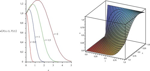
The important space–time coordinates of the solutions are given in Figure 3, which presents a heavy spreading out of the contaminant in space to time $t=\mathrm{2.0.}$

Remark 4.1:

For the experiments, we obtain full accuracy based on the analytical solution of the method. In comparison to standard numerical solvers, for example, finite volume methods, which is done for such related problems in [23], we obtain numerical errors about $er{r}_{FV}={10}^{-2}-{10}^{-4}.$We implement the solvers to a MATLAB^® code and deal with a standard PC, see also [36]. The computational time of the experiments lies in seconds, while comparison to standard numerical solvers lies in minutes, such that we gain a factor of 10 times. For further discussions to the benefits it can be found in [27].

Remark 4.2:

We applied the analytical solutions to the 1D macroscopic convection–diffusion–reaction equation. We see that the solution is resolved with respect to the time-dependency of the convection and diffusion part. Figure 3 shows the fast expansion of the solution in the space–time coordinate system with later times.

4.2. Systems of spatially dependent convection–diffusion–reaction equations coupled with a multiphase flow in four components

In the following experiment, we deal with a fully modelled macroscopic model, which is discussed in Section 2.2.1.

The numerical experiment is discussed with two components in [37]; here, we have enlarged the results for four components.

Here, we see the realistic behaviour of a quickly reacting exchange between the mobile and immobile phases, such that the concentration of the pollutants will fill up the immobile areas, as seen in Figure 2 with the mobile and immobile domains.

Such experiments are very important for seeing how a waste disposal scenario will contaminate the underlying rock or solid area, see [22]. Another modelling is to see the spreading out of deposited areas in chemical vapour depositions; here, there are also areas of immobile zones, which restrict the deposition to the correct mobile areas, see [38].

To simulate such spatial behaviour of an spreading out into an immobile area, we treat the following systems of spatially dependent convection–diffusion equations with mobile and immobile phases as given for porous media problems in [1,22]:

(93) $\begin{array}{rll}& {\mathrm{\partial }}_t{u}_i-D_i(x,t){\mathrm{\partial }}_{xx}{u}_i+{\upsilon }_i{\mathrm{\partial }}_x{u}_i=-{\lambda }_i{k}_i(t)u_i+\beta (g_i-u_i),& x,t\in [0,L]\times [0,t_{end}],\end{array}$(93)

(94) ${\partial }_t{g}_i=-{\lambda }_i{k}_i(t)\beta (g_i-u_i),x,t\in [0,L]\times [0,t_{end}],$(94)

where we have $i=1,\dots ,4.$ We have $D_i(x,t)=D_{0,i}(1+a_{i}x{)}^2,$ ${\upsilon }_i(x,t)={\upsilon }_{0,i}(1+a_{i}x),$ $k_i(t)=1.$ Further we have $D_{0,1}=1.0,D_{0,2}=0.5,D_{0,3}=0.3,D_{0,4}=0.2,$ ${\upsilon }_{0,1}=1.0,{\upsilon }_{0,2}=0.5,$ ${\upsilon }_{0,3}=0.3,{\upsilon }_{0,4}=0.2,a=a_0=a_1=1.0,{\lambda }_1={\lambda }_2={\lambda }_3={\lambda }_4=0.01,\beta =\mathrm{0.01.}$ The dimensions are given by $L=1,t_{end}=\mathrm{1.0.}$

We have to deal with at least two equations which are coupled via the B operator.

We transform this into linear convection–diffusion–reaction equations, as in Section 3.1:

(95) $Z=-log(aX)=log(1+ax),$(95)

and we obtain a steady-state solution with transient regimes, which are the inhomogeneous equations, and they are given as:

(96) $\begin{array}{rl}{\mathrm{\partial }}_t{u}_i=& a^2{D}_{0,i}{\mathrm{\partial }}_{ZZ}{u}_i-(a{\upsilon }_{0,i}-a^2{D}_{0,i}){\mathrm{\partial }}_Z{u}_i\\ & -(a{\upsilon }_{0,i}+{\lambda }_i)u_i+\beta (g_i-u_i),& Z,t\in [0,Z_0]\times [0,t_{end}],\end{array}$(96)

(97) ${\partial }_t{g}_i=-{\lambda }_i{g}_i-\beta (g_i-u_i),Z,t\in [0,Z_0]\times [0,t_{end}],$(97)

(98) $u_i(Z,0)=1,0\le Z\le Z_0=\log (1+aL),$(98)

(99) $g_i(Z,0)=0,0\le Z\le Z_0=\log (1+aL),$(99)

(100) $u_i(0,t)=g_i(0,t)=0,u_i(Z_0,t)=g_i(Z_0,t)=0,t>0,$(100)

(101) $i=1,2,3,4.$(101)

From the inhomogeneous equations of (96)–(101), we can derive the homogeneous equations, which are given as:

(102) $\begin{array}{rl}{\mathrm{\partial }}_t{u}_{hom,i}=& a^2{D}_{0,i}{\mathrm{\partial }}_{ZZ}{u}_{hom,i}-(a{\upsilon }_{0,i}-a^2{D}_{0,i}){\mathrm{\partial }}_Z{u}_{hom,i}\\ & -(a{\upsilon }_{0,i}+{\lambda }_i+\beta )u_{hom,i},& Z,t\in [0,Z_0]\times [0,t_{end}],\end{array}$(102)

(103) ${\partial }_t{g}_{hom,i}=-({\lambda }_i+\beta )g_{hom,i},Z,t\in [0,Z_0]\times [0,t_{end}],$(103)

(104) $u_i(Z,0)=1,0\le Z\le Z_0=\log (1+aL),$(104)

(105) $g_i(Z,0)=1,0\le Z\le Z_0=\log (1+aL),$(105)

(106) $u_i(0,t)=g_i(0,t)=0,u_i(Z_0,t)=g_i(Z_0,t)=0,t>0,$(106)

(107) $i=1,2,3,4.$(107)

For the homogeneous equations (102)–(107), we derive the analytical solutions, discussed in Section 3. Then the homogeneous solutions u_hom,i are

(108) $\begin{array}{rl}& u_{hom,i}(Z,t)=u_{0}exp(\frac{\upsilon }{2D}Z-\frac{{\upsilon }^2}{4D}t)exp(-\mu t)\sum _{j=1}^J\left({\psi }_{j,i}(Z)exp(-v_{j,i}t)f_{j,i}\right)+u_1{F}_i(Z),\end{array}$(108)

(109) $i=1,2,3,4,$(109)

where $u_0=1,u_1=1,$ the parameters are given by ${\upsilon }_i=a{\upsilon }_{0,i}-a^2{D}_{0,i},D_i=a^2{D}_{0,i},$ ${\mu }_i=a{\upsilon }_{0,i}+{\lambda }_i+\beta$ and the variables are given by

$f_{j,i}=\left(-v_{j,i}(cos(v_{j,i})-1)-\frac{{\upsilon }_i}{2D_i}sin(v_{j,i})\right)4\sqrt{2}$

(110) $\frac{D_i^2}{{\upsilon }_i^{2}4D_i^2{v}_{j,i}^2}exp(-\frac{{\upsilon }_i}{2D_i}),$(110)

(111) ${\psi }_{j,i}(Z)=\sqrt{2}sin(v_{j,i}Z),v_{j,i}={\beta }_{j,i}\sqrt{D_i},{\beta }_{j,i}=j\pi ,\mathrm{f}\mathrm{o}\mathrm{r}j=1,2,\dots ,J,$(111)

(112) $F_i(Z)=\frac{1-exp\left(-\frac{{\upsilon }_i}{D_i}(Z_0-Z)\right)}{1-exp(-\frac{{\upsilon }_i}{D_i})},$(112)

with $J=5,10,20,$ which are the number of the summation index for the approximated solution. We obtain a numerical accuracy based on that choices with $er{r}_{J=5}={10}^{-3},$ $er{r}_{J=5}=5{10}^{-4}er{r}_{J=5}=1{10}^{-4},$ see [30].

Furthermore, we have

(113) $Z=log(1+ax)$(113)

(114) $Z_0=log(1+aL)$(114)

(115) $D_i=a^2{D}_{0,i},{\upsilon }_i=(a{\upsilon }_{0,i}-a^2{D}_{0,i}),{\mu }_i=a{\upsilon }_{0,i}+{\lambda }_i+\beta .$(115)

The homogeneous solutions g_hom,_i are given by

(116) $g_{hom,i}(Z,t)=g_i(Z,0)\mathrm{e}\mathrm{x}\mathrm{p}(-({\lambda }_i+\beta )t)$(116)

(117) $i=1,2,3,4.$(117)

In the following, Algorithm 4.3, we apply the variation of constants, see [39], to obtain the solution of (96)–(101).

Algorithm 4.3:

On the time interval [0, t], one solves the following subproblems consecutively, for $j=1,2,3,...M$ and for the components$i=1,...,m.$

(118) $\begin{array}{rl}{u}_{i,j}(Z,t)=& u_{i,hom}(Z,t)\\ & +{\int }_0^t{u}_{i,hom}(Z,t-s)\beta g_{i,j-1}(Z,s)ds\\ & with{u}_{i,j}(Z,0)=u_{i,hom}(Z,0),\end{array}$(118)

(119) $\begin{array}{rl}{g}_{i,j}(Z,t)=& g_{i,hom}(t)\\ & +{\int }_0^t{g}_{i,hom}(t-s)\beta u_{i,j-1}(Z,s)ds\\ & with{g}_{i,j}(Z,0)=g_{i,hom}(0),\end{array}$(119)

where the initialization u_i,₀ (Z, t), g_i,₀ (Z, t) is an approximation of u_i(x, t), g_i(x, t) and can be chosen in this linear case to be 0, for example, the homogeneous solutions $j=6$ and $g_{i,0}(Z,t)=g_{i,hom}(Z,t).$ For the integrals, quadrature rules are employed, which have to be of order O(t^j), where $j=1,2,3,...$ are the iterative steps.The algorithm is finished after 2–5 iteration steps, or after a sufficiently small error:

(120) $\begin{array}{rl}& \underset{i=1}{\overset{m}{max}}\left(|u_{i,coupled,j+1}(Z,t)-u_{i,coupled,j}(Z,t)|,\right. \\ & \left. |g_{i,coupled,j+1}(Z,t)-g_{i,coupled,j}(Z,t)|\right)\le err.\end{array}$(120)

The retransformation is done by $(Z,t)\to (X,t).$

In the following, we study the numerical accuracy based on the different iterative steps:

• $j=1,2,3,...$ (number of iterative steps for the mobile–immobile coupling): Accuracy of the iterative method to couple the equations.

• $J=10,20,100$ (number of summation terms for the analytical solution): Accuracy of the analytical solutions of the mobile part of the coupled equations.

Figure 4 gives the analytical solutions of the mobile species of the coupled convection–diffusion–reaction equations.

Remark 4.4:

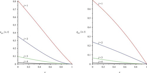
For the numerical accuracy, the optimal coupling results from at least $j=6$ iterative steps between the mobile and immobile solution. Further the analytical treatment of the mobile solution based on a summation of functions (see Section 3.1) needs at least $J=50$ for an optimal accuracy of 10⁻⁴, see Figure 5.

Figure 4. Numerical experiment for mobile species and the coupled analytical solution of the coupled convection–diffusion–reaction equations (2D plot: on left (mobile species), on the right (immobile species), j equals from one to six iterative coupling steps; J is from 10 to 50 iterative steps of the analytical solution).

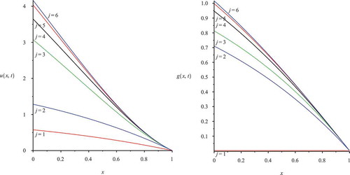
Figure 5. Contour 2D plot with $J=10,50$ analytical wave function and their improvements in the mobile (left figure) and immobile solution (right figure).

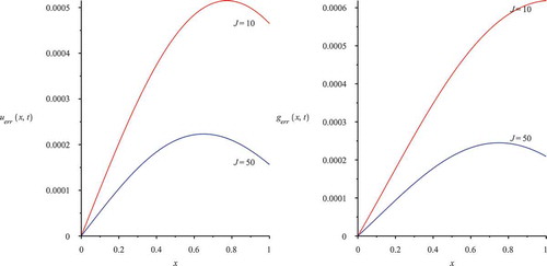
In Figure 5, we study the improvement in accuracy from using different numbers of iterative steps J for the analytical solutions of the mobile and immobile species of the coupled convection–diffusion–reaction equation.

In Figure 6, we study the improvement in accuracy from using different numbers of coupling steps j for the solutions of the mobile and immobile species of the coupled convection–diffusion–reaction equation.

Figure 6. Contour 2D plot with $j=1,4$ analytical wave function and their improvements in the mobile (left figure) and immobile solution (right figure).

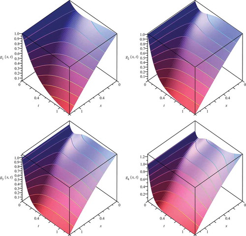
The analytical solutions of the mobile and immobile species of the mobile and immobile species of the coupled convection–diffusion–reaction equation are given in Figures 7 and 8. The concentrations of the mobile species are instantaneously exchanged to the immobile species, which means the pollution is contaminating the underlying solid (the immobile zones of the porous medium).

Remark 4.5:

For the experiments, we obtain a maximal accuracy of $er{r}_{J=100}={10}^{-4},$ where number of approximation terms is $J=100.$ In comparison to standard numerical solvers, for example, finite volume methods, with for example 100 spatial and 100 time-points, we have much more computational amount and we receive the numerical accuracy of $er{r}_{FV}={10}^{-2},$ see the numerical comparison in [16,23]. We achieve the same accuracy of about $er{r}_{FV}={10}^{-4},$ when we apply 100,000 spatial and 1000 time-points. Such that we have at least a factor of 10 times faster processes with the underlying analytical methods as for a numerical standard discretization method. The benefits of the analytical approach via the numerical standard discretization schemes can also be found in [23,27].

Remark 4.6:

In the results, we have presented the numerical convergence results with from three to five iterative coupling steps and sufficiently many, $J=100,$ analytical wave functions. The solutions are for mobile and immobile coupled problems. We see it has totally spread out into the immobile area, which means the parabolic solution in the time–space coordinate in Figures 7 and 8 is penetrating the full solid area. The mobile and immobile species exchange their concentrations based on their fast reaction scale, while we see a slower decay in their pollution. Here we see the importance of modelling such mobile and immobile phases, while we obtained a loss of the mobile concentrations by their passing into the immobile concentrations, which means the immobile reservoir of the underlying porous medium retards the contamination.

Figure 7. Numerical experiment for the mobile species of the analytical solution of the coupled convection–diffusion–reaction equations (3D plots with upper figures are the mobile solutions; lower pictures are immobile solutions), where we apply $j=6$ and $J=100$.

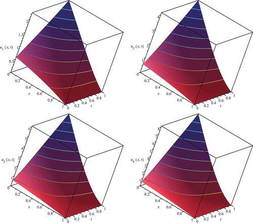
Figure 8. Numerical experiment for the immobile species of the analytical solution of the coupled convection–diffusion–reaction equations (3D plots with upper Figures are the mobile solutions; lower pictures are immobile solutions), where we apply $j=6$ and $J=100$.

5. Conclusions

The novelty was the application of a homogenization and multiscale approach to a model of a porous medium. We derived a fully macroscopic model of a two-phase model in a porous medium aquifer. It is important to apply a multiscale approach after the homogenization of the spatial scales to resolve also the time-dependencies of the underlying multiscale model. We derived 1D analytical solutions of the convection–reaction equations, which were then incorporated into the iterative approaches. The multiscale modelling approach allows reformulating and decomposing such delicately coupled systems of convection–diffusion–reaction equations. So for complex computations of large systems of space- and time-dependent convection–diffusion–reaction problems, an acceleration of the solver process is possible with a novel homogenized and upscaled model problem.

In the future, such combinations of multiscale modelling with underlying splitting approaches will be important for solving large systems of convection–diffusion–reaction equations where locally 1D analytical solutions of some of the subproblems can be embedded. For real-life applications in porous media modelling, such hierarchical models can be applied to circumvent expensive microscopic models.

Disclosure statement

No potential conflict of interest was reported by the author.

References

- M. Lieberman and A. Lichtenberg, Principle of Plasma Discharges and Materials Processing, 2nd ed., Hoboken, NJ : John Wiley & Sons Inc., 2005.
- J. Bear, Dynamics of Fluids in Porous Media, American Elsevier, New York, 1972.
- J. Bear and Y. Bachmat, Introduction to Modeling of Transport Phenomena in Porous Media, Kluwer, Dordrecht, The Netherlands, 1991.
- K. Westerterp, W. Van Swaaij, and A. Beenackers, Chemical Reactor Design and Operation, Netherlands University Press, Amsterdam, 1963.
- Z. Zlatev, Computer Treatment of Large Air Pollution Models, Kluwer, Dordrecht, The Netherlands, 1995.
- J. Geiser and M. Arab, Modeling, optimization and simulation for chemical vapor deposition, J. Porous Media 12 (9) (2009), pp. 847–867. doi:10.1615/JPorMedia.v12.i9
- A. Bellouquid and C. Bianca, Modelling aggregation-fragmentation phenomena from kinetic to macroscopic scales, Math. Comput. Model 52 (2010), pp. 802–813. doi:10.1016/j.mcm.2010.05.010
- C. Bianca and C. Dogbe, A mathematical model for crowd dynamics: Multiscale analysis, fluctuations and random noise, Nonlinear Stud. 20 (2013), pp. 349–373.
- C. Bianca, Modeling complex systems by functional subsystems representation and thermostatted-KTAP methods, Appl. Math. Inf. Sci. 6 (2012), pp. 495–499.
- E. Weinan, Principle of Multiscale Modelling, Cambridge University Press, Cambridge, 2010.
- J. Geiser, Multiscale splitting method for the Boltzmann–Poisson equation: Application to the dynamics of electrons, Int. J. Differential Equations. 2014 (2014), Article ID 178625, pp. 1–8. doi:10.1155/2014/178625
- J. Geiser, Modelling and simulation in engineering with multi-physics and multiscale methods: Theory and application, in Computational Methods for Engineering Technology, B.H.V. Topping and P. Ivanyi, eds., Saxe-Coburg Publications, Stirlingshire, Scotland, 2014, pp. 157–190.
- J. Geiser, Iterative Splitting Methods for Differential Equations, CRC Press, Chichester, England, 2011.
- J. Geiser, Multi-Scale Methods for Transport Problems: Theory and Applications, Cicil-Comp Press and Saxe-Coburg Publications, Review Paper, Special Issue, Stirling, UK, 2014. Accepted June 2014.
- L. Reifschneider, Solving inflow–outflow problems with functional splitting, in Proceedings of the American Institute of Aeronautics and Astronautics 22nd Meeting of the Aerospace Sciences, AIAA Association, Reno, NV, Jan 9–12, 1984.
- J. Geiser, Discretization methods with embedded analytical solutions for convection–diffusion dispersion–reaction equations and applications, J. Eng. Math. 57 (2007), pp. 79–98. doi:10.1007/s10665-006-9057-y
- M.H. Holmes, Introduction to Perturbation Methods, Texts in Applied Mathematics, Springer-Verlag, Berlin, 2012.
- A. Mikelic and C. Rosier, Modeling solute transport through unsaturated porous media using homogenization I, Computational Appl. Math. 23 (2–3) (2004), pp. 195–211. doi:10.1590/S0101-82052004000200006
- L.C. Evans, Partial differential equations, in Graduate Studies in Mathematics Vol. 19, AMS, Americal Mathematical Society, Providence, RI, 1998.
- U. Hornung, W. Jäger, and A. Mikelic, Reactive transport through an array of cells with semi-permeable membranes, Math. Modelling Numer. Anal. 28 (1994), pp. 59–94.
- A.E. Scheidegger, General theory of dispersion in porous media, J. Geophys. Res. 66 (1961), pp. 3273–3278. doi:10.1029/JZ066i010p03273
- E. Fein, Software Package r3t: Model for Transport and Retention in Porous Media, Final Report, GRS-192, Gesellschaft für Anlagen und Reaktorsicherheit, Braunschweig, Germany, 2004.
- J. Geiser, Discretisation Methods for Systems of Convective–Diffusive Dispersive–Reactive Equations and Applications, Monograph, Series: Groundwater Modelling, Management and Contamination, Nova Science Publishers, New York, 2008.
- J. Geiser, Model order reduction for numerical simulation of particle transport based on numerical integration approaches, Math. Comput. Model. Dyn. Syst. 20 (4) (2014), pp. 317–344. doi:10.1080/13873954.2013.859159
- W.A. Jury and K. Roth, Transfer Functions and Solute Movement through Soil, Bikhäuser Verlag, Basel, 1999.
- M. Genuchten, Convective–dispersive transport of solutes involved in sequential first-order decay reactions, Comput. Geosciences 11 (2) (1985), pp. 129–147. doi:10.1016/0098-3004(85)90003-2
- A. Kumar, D. Kumar-Jaiswal, and N. Kumar, Analytical solutions of one-dimensional advection–diffusion equation with variable coefficients in a finite domain, J. Earth Syst. Sci. 118 (5) (2009), pp. 539–549. doi:10.1007/s12040-009-0049-y
- J. Geiser, Discretization methods with analytical characteristic methods for advection–diffusion–reaction equations and 2D applications, ESAIM: Math. Modelling Numer. Anal. 43 (6) (2009), pp. 1157–1183. doi:10.1051/m2an/2009033
- Y. Sun, J. Petersen, and T. Clement, Analytical solutions for multiple species reactive transport in multiple dimensions, J. Contam. Hydrol. 35 (1999), pp. 429–440. doi:10.1016/S0169-7722(98)00105-3
- J.S. Pérez Guerrero, L.C.G. Pimentel, T.H. Skaggs, and M.T. van Genuchten, Analytical solution of the advection–diffusion transport equation using a change-of-variable and integral transform technique, Int. J. Heat Mass Transf. 52 (2009), pp. 3297–3304. doi:10.1016/j.ijheatmasstransfer.2009.02.002
- MATHEMATICA. Platform for Symbolic and Numerical Computations, Wolfram Research, Inc., Champaign, IL, 2015.
- G.A. Pavliotis and A.M. Stuart, Multiscale Methods: Averaging and Homogenization, Springer-Verlag, Berlin, 2008.
- B. Shivamoggi, Perturbation Methods for Differential Equations, Birkhäuser, Basel, 2003.
- F.J. Leij, N. Toride, and M.T. vanGenuchten, Analytical solutions for non-equilibrium solute trans- port in three-dimensional porous media, J. Hydrol 151 (1993), pp. 193–228. doi:10.1016/0022-1694(93)90236-3
- J.D. Cole, On a quasi-linear parabolic equation occurring in aerodynamics, Quart. Appl. Math. 9 (1951), pp. 225–236.
- J. Jürgen Geiser, Computing exponential for iterative splitting methods: Algorithms and applications, J. Appl. Math. 2011 (2011), Article ID 193781, pp. 27.
- J. Geiser, Modelling approach for mobile and immobile transport problems with multiple time-scales, IFAC-PapersOnLine 48 (1) (2015), pp. 635–639. doi:10.1016/j.ifacol.2015.05.002
- J. Geiser and M. Arab, Simulation of chemical vapor deposition: four-phase model, Spec. Top. Rev. Porous Media 3 (1) (2012), pp. 55–68. doi:10.1615/SpecialTopicsRevPorousMedia.v3.i1
- J. Geiser, Mobile and immobile fluid transport: Coupling framework, Int. J. Numer. Methods Fluids 65 (8)(2011), pp. 877–922. doi:10.1002/fld.2225