
 ?Mathematical formulae have been encoded as MathML and are displayed in this HTML version using MathJax in order to improve their display. Uncheck the box to turn MathJax off. This feature requires Javascript. Click on a formula to zoom.
ABSTRACT
A time-dependent two-scale multiphase model for precipitation in porous media is considered, which has recently been proposed and investigated numerically. For numerical treatment, the microscale model needs to be finely resolved due to moving discontinuities modelled by several phase-field functions. This results in high computational demands due to the need of resolving many such highly resolved cell problems in course of the two-scale simulation. In this article, we present a model order reduction technique for this model, which combines different ingredients such as proper orthogonal decomposition for construction of the approximating spaces, the empirical interpolation method for parameter dependency and multiple basis sets for treating the high solution variability. The resulting reduced model experimentally demonstrates considerable acceleration and good accuracy both in reproduction as well as generalization experiments.
1. Introduction
The present paper develops and shows numerically the efficiency of a model reduction scheme for a time-dependent two-scale model for a precipitation process in a porous medium that was recently introduced in [Citation29]. A porous medium is a domain that is perforated by so-called grains, cf. [Citation4]. The domain of interest is the pore space, which is the complementary domain to the union of the grains. The considered situation in [Citation29] and here is the following one. The pore space is occupied by a mixture of three substances: water, oil and a precipitate (e.g. salt). The water contains dissolved (salt) particles that precipitate on the grain boundary and form a crystalline solid if the concentration of the dissolved particles in the water exceeds a certain threshold. The reverse reaction is also possible, that is particles of the precipitate dissolve in the water if the concentration in the water is below this threshold. Therefore, the boundary between water and precipitate is a-priori unknown and moved besides curvature effects by precipitation and dissolution. The location of the boundaries water–oil and oil–water is also a-priori unknown but only driven by curvature effects, since it is assumed that particles of the precipitate cannot dissolve in oil and that water and oil are immiscible and incompressible. The evolution of the concentration of the particles in the water is driven by the precipitation process but also by diffusion.
Since the spatial scale of the diffusion process is much larger than the scale of the pores on which a phase transition takes place, the model of [Citation29] consists of two spatial length scales: a macroscopic so-called Darcy scale and a microscopic so-called pore scale. It was developed by the application of a homogenization technique to a pure pore-scale model for simplifying the numerical treatment; for an introduction to homogenization in porous media, see [Citation8]. In the two-scale model, the unknown on the macroscopic scale is the concentration of the dissolved particles in the water, and on the microscopic scale, the evolution of the phase boundaries is modelled by three phase-fields; see [Citation8,Citation9] for a general introduction to phase-field modelling with one phase-field,[Citation6,Citation7] for the handling of three phase-fields and [Citation8] for the diffuse domain approximation method that is used in [Citation29] in order to model the evolution of the characteristic functions of the three pore-space’s subdomains that are each occupied by one of the three constituents, water, oil and precipitate. Furthermore, an auxiliary function on the microscale is described that results from the upscaling and which acts as a microscopic correction of the diffusion tensor in the evolution equation for the macroscopic concentration. The two scales are coupled, that is the evolution of the phase-fields is influenced by the macroscopic concentration of dissolved particles in the water, and conversely, the evolution of the macroscopic concentration is influenced by the rate of microscopic precipitation and the microscopic auxiliary function.
The usual two-scale model’s (detailed/high-dimensional) discretization (as described in [Citation29]) consists of an evolution scheme for the concentration on a macroscopic numerical grid and for every macroscopic grid point of a microscopic cell problem describing the evolution of the three phase-fields and of the auxiliary function. The number of cell problems that must be solved in course of a simulation is equal to the product of the number of macroscopic nodes times the number of time steps. This soon becomes numerically very demanding if both numbers increase, since in order to solve a cell problem accurately, a fine discretization is necessary.
The present study presents a model reduction approach for the two-scale model described above. Existing approaches dealing with model reduction for multiscale problems involve reduced basis approaches for cell problems [Citation5, Citation22, Citation24], the localized reduced basis multiscale method [Citation20,Citation2] or kernel surrogate models for microscale models [Citation14]. While the former are used in the context of linear problems, the latter allows nonlinear problems but only is applicable in the case of few number of inputs/outputs in the coupling of the scales.
Our approach is projection-based and aims at a reduction of the most expensive part of the cell problems in order to accelerate the computation of the overall two-scale model, where it is the discretization of the auxiliary function that is most expensive. The problem for the auxiliary function strongly depends on the shape of the microscale subdomain occupied by the water, that is the problem depends on the phase-field modelling this subdomain. The problem is elliptic but, since the phase-field for water evolves in course of a simulation, it is implicitly time-dependent, that is a good approximation of complete trajectories and a high solution variability must be accounted for by the reduction approach. In [Citation28], a similar procedure was developed for a two-scale model for crystal growth.
The detailed model for the auxiliary function will be projected to a low-dimensional solution subspace generated via a proper orthogonal decomposition (POD; [Citation19,Citation30]) strategy based on high-dimensional snapshots. The empirical interpolation method (EIM, [Citation3,Citation15]) deals with the parameter dependency enabling to evaluate local parametric discretization operators efficiently. In particular, we refer to the empirical operator interpolation approach for linear and nonlinear operators [Citation11,Citation17], as well as the discrete empirical interpolation method (DEIM) for nonlinear parametric ordinary differential equations [10] or extensions as the matrix DEIM used in [Citation33]. In addition to full precomputation of the offline data, recently also online adaptation procedures have been introduced that accept online complexities linear in the full dimension H and continuously update the reduced model throughout the simulation [2,26]. As last step in our reduction, the reduced models are subdivided into submodels where each of them is capable of producing accurate low-dimensional approximations to the high-dimensional solutions for certain shapes of the water domain. Local subdomain basis approaches can also be found in other articles on model order reduction [1, 12, 13, 16, 25, 31], where time, parameter or state–space distance is used as partitioning criterion. As an alternative to partitioning, also interpolation of local models is a possible approach, for example [14]. But here, we follow the partitioning idea and the utilized partitioning criterion will be the volume of the precipitate.
The paper is structured as follows. Section 2 will present the detailed two-scale model as introduced in [29] and additionally gives a matrix-based formulation of the microscale problem that will be reduced. This microscale equation then is subject to a POD/EIM-based model reduction, which is explained in Section 3. The extensive Section 4 then presents numerical results, which illustrate the efficiency of the reduced model over the full model both in reproduction, as well as generalization settings. The paper is concluded with comments in Section 5.
2. The detailed two-scale model
This section briefly discusses the detailed discrete two-scale model describing the evolution of the dissolved particles’ concentration in the water phase on a Darcy-scale (macroscopic) and the evolution of the boundaries of the three substances, water, oil and the precipitate, on a pore-scale (microscopic) of a porous medium. Note that this description will be very concise only focussing on the relevant parts for the derivation of our subsequent reduced model. A detailed development and explanation of the model is presented in [Citation29]. The model consists of a macroscopic homogenized equation modelling the evolution of the concentration u of the dissolved particles in water, and at each point of the macroscopic domain of microscopic cell-problems with periodic boundary conditions modelling the evolution of the three substances and of two auxiliary functions w1 and w2. The evolution of the substances is modelled by three phase-fields which smoothly approximate the characteristic functions (in a sharp-interphase sense) of the three subdomains occupied each by one of the substances.
Consider a time-interval J(T): = [0,T] with the end time T > 0 and , a macroscopic spatial domain
of dimension d = 2 with a boundary
and a microscopic spatial domain Y = (0,1)d. The domain Y is subdivided into a pore-space
, a grain
and the grain’s boundary
, that is
. The boundary
of the pore-space
equals
. Let nΩ be the outer-normal to
and
the inner-normal to
.
As mentioned above, the pore-space is occupied by three substances Pi, iμI = {1,2,3}: two immiscible, incompressible fluids P1 (water) and P2 (oil) and the precipitate P3. In a sharp-interface setting, the substances would occupy three disjoint time-dependent a-priori unknown regions
,
and
. In the phase-field setting considered in this article, three phase fields smoothly approximate the characteristic functions
,
and
of
,
and
, that is for iμI = {1,2,3}, the phase-field smoothly approximates
. The model ensures a perfect mixture of the three phase fields
in the sense that their sum equals 1 and each of them is not less than 0, that is
.
In the considered initial configuration, μ of the three phases, depicted in , the precipitate P3 surrounds the grain which is located in the centre of the microscopic domain Y, the fluid P2 is located in the corners of Y and the fluid P1 occupies the remainder of the pore-space . Due to the considered periodic boundary conditions onμY, both P2 and
are spherical, where P3 is perforated by the grain.
Figure 1. The considered initial configuration ℐ of the three substances in the microscopic pore-space μ, where . The grain μ is located in the centre of Y and the pore-space μ is occupied by the two immiscible and incompressible fluids P1 (water) and P2 (oil) as well as the precipitate P2. The spherical perforated precipitate P3 is attached to the boundary Гμ of the grain μ, the spherical fluid P2 domain is located in the corners of the microscopic domain Y and the fluid P1 occupies the remainder.
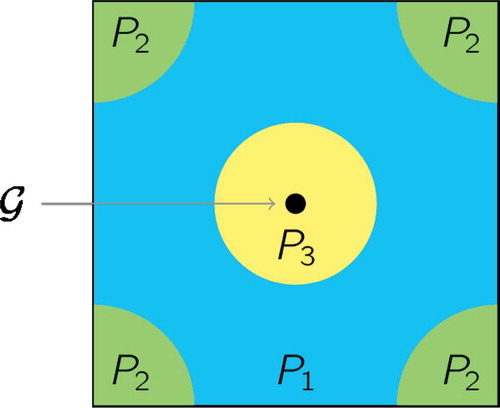
The fluid P1 contains dissolved particles that can precipitate on the grain-boundary Гμμ as well as on the boundary of an already existent precipitate μμP1. By assumption, P2 cannot contain particles, hence the concentration is 0 in P2. Furthermore, ρ > 0 is the fixed concentration of particles in the precipitate region P3.
The upscaled model considered here is derived in [Citation29] by a homogenization technique from a pure microscopic model for the concentration u and the phase-fields Φ for the idealized situation of periodically distributed grains. The cell problems for the auxiliary functions w1 and w2 result from the homogenization process.
2.1. The homogenized macroscopic equation for the concentration
In our presentation, we will use the notational convention that variables related to the partial differential equation model are put in normal font, independent of whether they are scalar or low-dimensional vectors. We then discriminate the resulting discretized high-dimensional coefficient vectors and matrices by consistently using an underline under the corresponding variable. The macroscopic spatial variable will be denoted by x ∈ Ω, the microscopic spatial variable by y ∈ Y. These are used as subscript for denoting the corresponding spatial differential operators, in particular . Applying these conventions, we can formulate the macroscopic equation for the concentration:
Problem 2.1: Given the diffusion coefficient , the fixed concentration
of particles in the precipitate P3 and the regularization parameter
, the microscopic field variables
and
and the initial conditions
, find the macroscopic concentration
satisfying
where the input of the microscopic variables is averaged on as follows:
with Kronecker’s delta , and where
The function approximates a linear function interpolating between 1 in a water–precipitate- and 0 in a water–oil-interface. Therefore, the last term on the left-hand side of the first equation in (1) accounts for the conservation of the particles’ mass.
Remark 2.2: The symmetry of the considered initial configuration ℐ of the three phases yields
in . A thorough investigation of the considered symmetry’s implications will be carried out in the Remarks 2.4 and 2.6.
2.2. The microscopic cell problems
The microscopic cell problems describe the evolution of the phase-fields Φ and the auxiliary functions w1 and w2.
Problem 2.3: Given the time-relaxation parameter α > 0, the parameter ξ > 0 that is proportional to the width of the phase transition regions, the parameters with
(where ρ > 0 is the fixed concentration of particles in the precipitate P3), the macroscopic field variable
, and the initial conditions
, for every x μμ Ω find the Y-periodic microscopic phase-fields
satisfying for i ∈ I
with the potentials
where
The function W(Φ) is non-convex in and minimal for the pure states
. Since γ13 is an indicator of the diffuse interface
between water and precipitate and
is an affine linear rate function with a given constant rate
and a constant threshold
that separates precipitation and dissolution, the forces f1 and f3 drive the precipitation process. If u is larger than
, then dissolved particles precipitate and the precipitate phase expands, otherwise it recedes if
.
Remark 2.4: Since the subspace of the admissible states of Φ is an invariant subspace of the solution operator
of Problem 2.3, it is sufficient to solve the problem for i = 2,3 and subsequently to set
, see [Citation29]. Furthermore, the considered initial configuration μ of the three phases satisfies for
in
.
To be precise, Φ is rotational symmetric of order 4: a rotation of Φ by an angle of 90 does not change it.
Problem 2.5: Given the diffusion coefficient D = 0 and the regularization parameters δ > 0, the microscopic field variable , for j = 1,2 for every x ∈ Ω find the Y-periodic microscopic solution
with vanishing average in μ satisfying
Remark 2.6: Since Problem 2.5 is completed by periodic boundary conditions, it is only uniquely solvable owing to the constraint demanding that the solution vanishes on average. Furthermore, due to the considered rotational symmetry of the three phases, the solutions satisfy
in J(T × Ω. Furthermore, is symmetric to the axis
and anti-symmetric to
. In combination with (9), these observations yield
Therefore, it is sufficient to solve Problem 2.5 for w1 only.
2.3. Discretization
Problems 2.1, 2.3 and 2.5 are discretized by the explicit Euler method with respect to the time, and by standard second-order finite differences on uniform rectangular grids Ωhg and Yhμ with respect to the spatial domain, where hg > 0 denotes the macroscopic and hμ > 0 the microscopic space-increment. The discrete microscopic pore-space μhμ is a subset of Yhμ. The time-increment μnt depends on , due to the CFL-condition for the discretization of Problem 2.1.
Since it is demanding to solve the microscopic cell Problems 2.3 and 2.5 in all macroscopic nodes, the problem is solved adaptively in the sense of [Citation27], that is only the microscopic problems in active macroscopic nodes are solved and the microscopic data of inactive nodes
is approximated. Details are also given in [Citation1]. This results in the following algorithm:
Algorithm 1:
Set n = 0,
and
Set n = n + 1 and
Adjust the set An of the active macroscopic nodes.
For every node in An solve the discretization of the microscopic Problem 2.5 for
For every node in
Approximate the microscopic parameters
Solve the discretization of the macroscopic Problem 2.1 for
Go back to Step 1 if tn = T.
In this algorithm, the computation of the elliptic problem for in Step 1 is the crucial expensive component – a detailed complexity discussion follows in Section 3. Therefore, only the microscopic Problem 2.5 for
will be solved in a reduced sense in the reduced two-scale model to be developed. The detailed model’s discretization of 2.5 reads
where and
is the set of first-order neighbours of
, that is
As this, problem will be reduced, a compactly written vector–matrix formulation is provided in the following, which is more accessible than the above detailed formulation. For this, define as the (high) dimension of the field variable
and introduce the vectors of degrees of freedom (DOF)
and
, assuming a suitable enumeration of μhμ. The auxiliary function
is characterized by the system of equations
where the matrix and the vector
depend linearly on the solution
of the microscopic Problem 2.3. To be precise, let
define the set of indices of the first-order neighbours of the node
and ri (and correspondingly μi) define the index of the first-order neighbour to the right (left) of the node i, then for all
the matrix and the right-hand side are given by
The solution of the system is approximated by a CG procedure with the following abort criterion: stop the iteration if the maximum norm of the residuum is less or equal than the product of the tolerance δ and the maximum norm of the right-hand side. A Lagrange-multiplier ensures uniqueness by enforcing the vanishing average.
3. The reduced two-scale model
The discretization of the microscopic Problem 2.3 describing the evolution of the phase-fields and
in each step of time in each active macroscopic node is solvable in
(H), and the complexity of the discrete macroscopic Problem 2.1 for u is insignificant. However, the complexity of solving the sparse linear system (15) for
in each step of time in each active macroscopic node is roughly
, if we assume a standard iterative solver, where the number of iterations as well as the cost for matrix–vector products grows linearly with H. Consequently, the overall complexity of the discrete two-scale model is reducible significantly by reducing the complexity of the model for w1. In the overall reduced two-scale model, operations of complexity
are accepted. Therefore, only the model for w1 is reduced, that is Step 1 of Algorithm 1 is replaced by
For every node in An approximate the high-dimensional solution
The reduced model must account for the dependency on a time-dependent parameter, that is it must provide a good approximation of complete trajectories and a high solution variability, and the coupling of the microscopic equations. To consider this, a POD for the trajectory treatment, EIM for the parametrization and a partitioning approach to account for different solution regimes will be applied. As we refer to [Citation28] at various places, we want to comment on the relation to that previous study in order to clarify the contribution of the current paper. The commonality to [Citation28] is that we also consider an instationary macroscopic two-scale problem that is coupled to multi-field microscopic models, where the microscopic models are reduced by POD/EIM and a partitioning approach resulting in multiple bases. But the fundamental difference of the current study to [Citation28] is that we have a completely different application setting (here precipitation in contrast to crystal growth), with different field variables, different equations and nonlinear coupling of the microscopic fields into the macroscopic model. This requires various changes in the methodology. In particular, we merely reduce the most costly component of the model, which is only one microscopic field variable, we leave other microscopic field variables unreduced.
As typical in parametrized model reduction procedures, the overall reduction process consists of an offline and an online phase. In the offline phase, the reduced basis and further quantities are pre-computed, this phase is accepted to be costly, but only performed once. The online phase of the reduced model then will be of low complexity and allows the reduced scheme to be used rapidly and multiply. We summarize these stages for our current problem in order to clarify the overall workflow from parameter inputs to solutions from the reduced two-scale model:
In the offline phase for a given parameter setting of the two-scale model (e.g. choice of initial values, boundary conditions, macro grid resolutions), we solve the full two-scale model for this training setting by Algorithm 1. During this computation, we collect snapshots for and the right hand side
for the construction of the reduced model for
. The construction of the corresponding basis and further offline quantities will be explained in Section 3.1.
In the online phase, for various parameter settings of the two-scale model, the two-scale model is solved by Algorithm 1 but using step (5ʹ) instead of step (5). This means, for all active macroscopic nodes, the macroscopic value un − 1 is used as input parameter into the microscopic model. More precisely, the pointwise value of enters the microscopic fields
and
, these determine
, which is the final field that enters the reduced model for the microscopic variable
. The detailed explanation of the computations for this reduced microscopic problem for the auxiliary variable w1 is given in Section 3.2. Then the suitably averaged microscopic fields enter the macroscopic evolution problem enabling the macroscopic timestep to obtain un. So, clearly, the reduced model for
is used multiply for all timesteps and all active macroscopic nodes and different macroscopic simulation runs by varying macroscopic parameter settings.
3.1. The offline phase
The following steps are processed in the offline phase.
Solve the detailed two-scale model and collect snapshots
of the microscopic solution
and of the right hand side
Construct a reduced basis Φw by POD:
Perform the offline phase of the Empirical Interpolation Method EIM [Citation3] to generate an approximation of the high-dimensional microscopic model (15). Use as training data the snapshot set
Furthermore, with respect to the five-point-stencil which discretizes the spatial derivatives, determine the indices
Determine the reduced operators which are required for solving the reduced model; details on the operators are given in the following.
Although these offline quantities comprise a reduced basis and the interpolation points, this set of quantities is denoted a reduced basis set
Similar as for a crystal growth model [Citation28], not only one but also many basis sets are used for different solution regimes. Aim of the reduction is to obtain an accurate solution in much less online time than needed for the detailed model. Accuracy increases with increasing numbers Nw, μYMμμ andμμYNMμμ. Contrary to this relation, speed of computation increases with decreasing numbers Nw, μYMμμ andμμYNMμμ. In order to keep those numbers low but still to gain accurate results, multiple basis sets are used. A problem-specific feature extraction is used to partitioning the solution space. The utilized criterion is the volume of the precipitate P3. Since the fluid domain for P2 is almost unchanged, microscopic configurations of the three phases with similar precipitates’ volumes are similar themselves. Similar configurations result in similar solutions w1,H.
The construction of the basis sets
in the offline and their usage in the online phase is now straightforward. The collected snapshots are partitioned into subsets for different subintervals of the precipitates volume. This is done such that the number of snapshots is (roughly) equal for each subset, and results in volume subintervals of different size, as will be demonstrated in the experiments. For each of these snapshot subsets, the steps (2), (3), (4) mentioned at the beginning of this subsection are performed in order to generate the basis set for each subinterval.
As known in local basis construction, it can be beneficial to guarantee a certain overlap of snapshot sets for local bases [Citation28]. Identical to [Citation28], we introduce an overlapping parameter , which extends the snapshot sets for an interval to cover some snapshots from both neighbouring intervals. In particular,
corresponds to the non-overlapping situation as just explained, while
implies a full inclusion of the snapshot sets for the previous and next interval. In practice, a value of the overlapping parameter will be chosen close to 0.
In the online phase, the volume of the local precipitate is computed, the corresponding subinterval is determined and the corresponding basis-set is then used for computing the reduced approximation of the microscopic field w1.
3.2. The reduced model for w1
The standard empirical interpolation system approximating the detailed system (15) for the auxiliary function reads
with and
, where the index YM denotes that only the rows of the matrices belonging to the magic points’ indices are considered, where
is the matrix with columns equal to the DOF-vectors of the current appropriate POD-basis Φw, and where
is the matrix with columns equal to the DOF-vectors of the current appropriate collateral basis
. This system is not suitable because a high-dimensional system must be solved in the online phase and, furthermore, it is unknown whether the system is of full rank and it is over-determined. Therefore,
is eliminated from the equation by a suitable biorthogonal matrix multiplication, resulting in
with a matrix and a vector
. This system is suitable for an online phase because it is low-dimensional. It is solved for
by a Least-Squares procedure via the pseudoinverse, as it still will be over-determined in general when
.
In correspondence to (15), the low-dimensional matrix and vector are defined as follows:
with defined as
and with the restriction-matrix defined as
The matrix is pre-computed in the offline phase. What remains to be computed in the online phase’s time-step
is
the sparse matrix
the vector
finally, the least-squares solution
All of these computations for the online phase of the reduced model are completely independent of the high dimension H. The computational complexity only scales with and
. Consequently, the reduced model for w1 provides an ideal offline/online decomposition.
However, in order to approximate the microscopic parameter in
in Step 6 of Algorithm 1 the high-dimensional solution
must necessarily be approximated, which is done by the reconstruction operation
of complexity linear in
. This complexity could also be reduced by involving an additional empirical interpolation step for this averaging equation. However, for our purposes, it is acceptable to have this moderate linear dependency on H in this coupling step.
4. Numerical results
This section presents numerical solutions of the two-scale problem for precipitation in porous media computed by the Algorithm 1 – with high-dimensional and reduced (i.e. low-dimensional) solutions of the auxiliary function w1. Three test settings S1, S2 and S3 in two spatial dimensions are considered, where S2 and S3 are variations of S1. Initially, reduced models are developed from high-dimensional snapshots of the setting S1 which therefore is the training setting. After demonstrating the significant efficiency gain of the reduced models in comparison to a high-dimensional discretization of S1, it is shown that the reduced models’ solutions of the settings S2 and S3 also approximate the corresponding high-dimensional solutions.
4.1. The three settings S1, S2 and S3
The varying parameters of the settings S1, S2 and S3 are specified in : the final time T of the time-interval, the number of the macroscopic nodes Hg in x1 and x2 direction, the initial macroscopic concentration u0, a function u_(t) that is relevant for the macroscopic boundary condition of u, and the precipitates’ initial radii r0. The following paragraph presents further explanations for the varying parameters and specifies the remaining common parameters of the three settings.
Table 1. The varying parameters of the three settings S1, S2 and S3, which are explained in Section 4.1 and . The function u_(t) = a:b increases linearly from a to b with the time-steps in the course of a simulation. For i = 1,2 an initial precipitate’s radius results in a precipitate’s initial portion of
on the overall pore-space’s volume, analogously the water’s initial portion is
, and the oil’s initial portion is
due to a radius
.
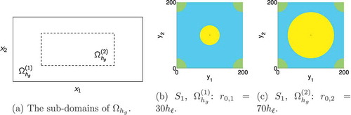
Figure 2. The initial phase configurations in the microscopic pore-space in the two subdomains
and
of the macroscopic domain
. The black points in the very centre of
in (b) and (c) represent the small spherical grains
. Each grain is surrounded by a precipitate
(yellow). For
,
defines the initial radius of the precipitates in the subdomain
. Each precipitate is surrounded by water (blue) and a spherical oil phase
(green) is located in the corners of
. The coloured subdomains Pi are characterized by
for
. Full colour available online.
The time interval is discretized by
using the time-dependent increments
, where
, which results from stability considerations. This δ is also used as error tolerance of the CG-method solving the high-dimensional elliptic system (15) for the auxiliary function
. The microscopic pore-space
is perforated by a small spherical grain
located in the centre of
and consisting of one node. Let H = 200 denote the number of the microscopic nodes in each space dimension. Then, the microscopic domain
and the pore-space
are given by
The edge-length of
defines the macroscopic space-increment
. The macroscopic domain
is defined as
The initial concentration and the diffusion coefficient
are fixed. For simplifying the numerical boundary treatment, it is assumed that Ω is surrounded by a virtual domain
of one cell row such that the mixture in Ω is surrounded by a virtual mixture in
. The diffusion tensor in a node
shall be the same as in the node
, which is the orthogonal projection of
on
that is the point with shortest distance to xy, ergo
. Hence, for
,
By definition, the concentration in the surrounding virtual domain Ωv yields on the one hand that dissolved particles flow into Ω across its upper and its right boundary and on the other hand that the remaining part of the boundary is not permeable. Precisely, for all , the concentration is defined as
The remaining microscopic physical parameters are prescribed as ,
, and the concentration of particles in the precipitate P3 satisfies
. The parameters of the rate-function f from (8) are fixed as
and
, that is dissolved particles precipitate if their concentration exceeds the threshold of
and contrarily, the precipitate dissolves if the concentration falls below 0.5. Due to the initial concentration
in setting S1, the precipitates dissolve in the beginning of the time-interval and grow again as soon as, due to the boundary condition, the concentration exceeds 0.5. On the contrary, the precipitates never dissolve in settings S2 and S3.
What remains to be specified is the initial configuration of the phase-fields and the parameters of the adaptive solution strategy. The grain is surrounded by a spherical precipitate P3 as displayed in . The fluid P2 is located in the corners of the microscopic domain Y. Due to the periodic boundary conditions, P2 is spherical with prescribed radius . The macroscopic domain
is subdivided into the two subdomains
and
, where
with the floor-function . By definition, the initial perforated spherical precipitates in
are of radius r0,1 and in
of r0,2. Finally, for completeness, the parameters of the adaptive solution strategy are specified as follows, see [Citation33]:
,
,
,
,
,
, IT-CA, the copy method; the initial set of active nodes contains, respectively, one node from both subdomains
and
, and the refining tolerance is defined as
where is a metric with a fading memory measuring the distance of the concentration evolution in two macroscopic grid points.
In each setting, the macroscopic concentration u does never and nowhere fall below u0 (initial condition) or exceed (boundary condition), that is
in the macroscopic time-space cylinder
. Therefore, due to similar initial microscopic conditions of the three settings, and since similar evolutions of the macroscopic concentration result in similar microscopic evolutions of the three phases Φ and hence of the auxiliary function w1, it is expectable that the reduced models developed from high-dimensional snapshots of setting
are capable of approximating the high-dimensional solutions of
and
, despite the fact that the macroscopic domains and the time-interval of the three settings vary significantly.
The quality of an approximation to a high-dimensional solution
is estimated by
(1) the -norm of
,
(2) the -norm of
,
(3) the -norm of
,
(4) and the -norm of
where the following abbreviations are used ,
. The term
defines the microscopic correction of the macroscopic diffusion tensor
of (5),
represents the macroscopic time-space cylinder and
represents a subset of the microscopic time-space cylinder.
contains every 100th step of time and
contains the macroscopic nodes highlighted in . The subset
instead of
is used to measure the microscopic quality because of the large number of the microscopic DOF and due to limitations of memory resources. However, since the microscopic solutions do not change significantly from one step of time to another one, and since the nodes of
are well distributed in the macroscopic grid
, an accurate approximation of the overall error can be expected.
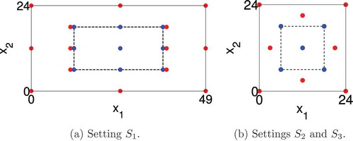
Figure 3. The nodes in the subset of the macroscopic grid
: nodes of
are indicated in red, and in blue those of
. Full colour available online.
4.2. Setting : the reproduction ability of the reduced models
Setting ’s high-dimensional solution at the final time
is depicted in and the evolution of the precipitates’ volume fractions in . The setting’s initial concentration
is below the threshold
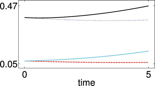
separating precipitation and dissolution. Therefore, in the beginning of the time-interval the precipitates dissolve and their portion on the pore-space’s volume decreases, and in contrast, the concentration of dissolved particles in the water increases inversely proportional. A further burst of growth of the concentration results from the boundary condition on the upper and the right boundary of
, that is from the prescribed increase of the concentration in the virtual mixture surrounding the mixture in
on top and on the right. As soon as the concentration exceeds the threshold
, dissolved particles precipitate and the precipitates’ volume portions increase. The edges in the macroscopic field
result from the strong diffusion in
and the weak diffusion in
. The larger the volume fraction of the water the stronger the diffusion of the dissolved particles on the macroscopic length scale. The shape of a microscopic field
is strongly influenced by the shape of the water-indicator
. In areas characterized by small absolute first derivatives of
, the auxiliary function
is almost constant. On the contrary, areas characterized by large absolute first derivatives of
are also characterized by large absolute values of
, where the sign of
and
is the same.
Figure 4. High-dimensional solution of setting at the end of the time-interval for
.
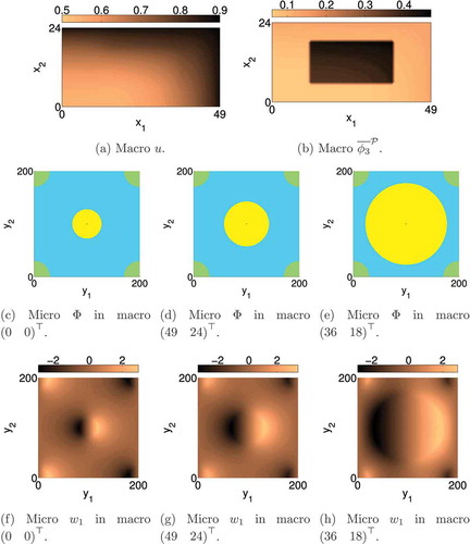
Figure 5. High-dimensional solution of the setting : the evolution of the precipitates’ volume portion on the pore-space in the macroscopic nodes
(red dashed),
(blue dotted),
(black) and
(cyan). In
the node
(and respectively,
) is host of the precipitate with the minimum (maximum) volume portion throughout the time-interval. The same relation holds in
for
(minimum) and
(maximum). Full colour available online.
Applying Algorithm 1 (high-dimensional), the solution has been computed by processors of type Intel(R) Xeon(R) CPU [email protected] GHz in roughly 57 h. On average, roughly
and in maximum
macroscopic nodes have been active that is the microscopic problems in these nodes have been solved. Consequently, in maximum every processor had to solve three high-dimensional microscopic problems per step in time and the number of steps in time was roughly
.
The reduced models are constructed from snapshots of the setting ’s high-dimensional solution. Every 16th step of time the solution
and the right-hand side
in every active macroscopic node are memorized. As explained earlier, the developed reduced models do not consist of only one but
reduced basis sets (with the overlapping parameter
), by the ultra-small tolerance
it is guaranteed that the number
of the magic points
is not smaller than the size
of the POD-basis
in each reduced basis set, such that the systems are not under-determined, and finally, the second stopping condition
assures that the number of the magic points is not much larger than the size of the corresponding POD basis.
tabulates results of six reduced models (,
,
,
,
and
) with varying tolerance
, where
in
(
, and of a high-dimensional approximation
with prescribed vanishing auxiliary function
. Since the high-dimensional solution’s macroscopic concentration
varies in the course of the simulation between
and
, the high-dimensional approximation
’s error of
is (at least) roughly
, which is not insignificant. It is roughly
(!) for the phase fields
. And the total error of
in the water region is
which at the same time is the maximum of
of the solution of the high-dimensional model that does not neglect the auxiliary function
. Therefore, approximating the high-dimensional solution by
results on the one hand indeed in a vast speed-up of the computation time, but on the other hand, its accuracy is unacceptable. This result indicates the need and is a justification for using the two-scale model including
instead of neglecting the quantity.
Table 2. Results for setting : the column entitled by ‘speed-up’ presents the rough speed-up of the approximations’ computation time in comparison to the high-dimensional solution of
in 57 h (as for the high-dimensional solution
processors of type Intel(R) Xeon(R) CPU [email protected] GHz were used), and the columns entitled by
,
,
and
present the approximations’ accuracy. The line entitled by
presents the results of a high-dimensional approximation with prescribed
resulting in
and
.
Almost the same speed-up as the model is gained by the reduced model
with
. Every error indicator shows that
is much more accurate than
. The weakest accuracy with a relative error of around
is observed by the indicator
measuring the error of the auxiliary function
in the water region. However, the results presented in show that for
each basis set consists of solely one POD mode (
) for
. Considering this, the accuracy is surprisingly high.
Table 3. Results for setting : the columns entitled by
,
and
present the average sizes of the
basis sets of a reduced model, and the column entitled by ‘reduction time’ presents the time that one processor of type Intel(R) Xeon(R) CPU [email protected] GHz needs to construct the reduced models from the pre-computed snapshots of the high-dimensional solution of
. In particular, this time is not the full offline time, as it does not include the 57-h for the snapshots computation.
The reduction of the POD-tolerance yields an increase of the mean number of POD modes, magic points and their neighbours. The increase of the mean number of POD modes and the mean number of magic points is roughly the same, due to the second stop condition for the procedure determining the magic points: it stops once the EI-error falls below
or
. The increase of the mean number of the magic points’ neighbours is a little weaker since some of them are magic points themselves. Summarizing, a decrease of the tolerance yields an increase of the basis sets’ sizes. The larger their sizes the more must be computed and the longer it takes. This is observed in both phases of the reduction procedure, that is in the part of the offline time for the reduced model construction from precomputed snapshots (, column ‘reduction time’) and the online phase (). A speed-up of
corresponds to an online computation time of roughly 0.3 h, and for
, it is 0.4 h. In comparison to the high-dimensional solution, this is a significant speed up.
What is even more important to observe than the modest deceleration of the computation time, is the fact that for the POD-tolerance tending to
the reduced converges to the high-dimensional solution. In fact, for the reduced model
with
, the errors of the macroscopic concentration
and of the phase-fields
vanish numerically. The error of the microscopic correction
of the macroscopic diffusion tensor
and of the auxiliary function
in the water region
are five orders of magnitude smaller than the error for
, which actually indicates a relative error of the same order.
As mentioned above, each two-scale model, that is both the high-dimensional and the reduced ones, are solved adaptively by Algorithm 1, where Step (5) is replaced by a reduced approximation (5ʹ) for the reduced two-scale model. As described in [29], the selection of the active macroscopic nodes is only determined with respect to the evolution of the concentration in the macroscopic nodes of
. Since, as tabulated in , the differences of the high-dimensional and the reduced models in the macroscopic concentration field are very small, the same nodes are active and consequently the same microscopic cell problems are solved in the high-dimensional and in the reduced simulations. Therefore, the adaptive strategy does not falsify the error estimates.
Note that indeed the problem of the moving phase boundary is a hard problem to reduce as it is “almost” a discontinuity. This is reflected in the requirement of many local bases for adequate approximation. Certainly, the overall sum of local basis sizes may be very well in the range or beyond the original full dimension. But still the model represents a valid reduced model, as each single microscopic model is approximated by a low-dimensional problem.
The presented results are a justification of the employed strategy constructing the reduced models, since they show the desired online speed-up and the reproduction ability: the reduced models can be solved much quicker than the high-dimensional model and their results are a good approximation to the high-dimensional ones.
shows for the macroscopic points ,
,
and
the evolution of the microscopic precipitate’s volume (a) and the corresponding evolution of the utilized basis set (b) in the reduced model
with
. The larger a precipitate’s volume the higher the index of the basis set used to approximate
. Important to note is that, despite the fact that the volumes in
and
are far from similar, the same basis set with index
is used in the end of the time-interval. This is due to the fact that
is host of the cell problem with the largest precipitate’s volume in the subdomain
and
hosts the smallest in
. The smallest in
is way larger than the largest in
, but the volume interval of basis set
contains both of them, which can also be seen in (a).
Figure 6. Results for the setting and the low-dimensional solution
with
: (a) presents the evolution of the precipitates’ volumes
and (b) the utilized basis sets in the course of the simulation in the macroscopic nodes
(red dashed),
(blue dotted),
(black) and
(cyan). Full colour available online.
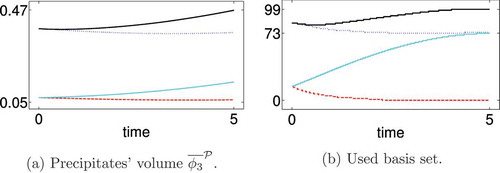
Figure 7. Results for the setting and the low-dimensional solution
: (a) depicts the minimum (black) and maximum (cyan) of the volume interval for the precipitates for the
basis sets that are used in the online phase to determine the proper basis set in order to approximate the reduced solution of
, where the minimum is
for basis set
and the maximum is
for basis set
; (b) shows the number of POD modes (cyan) and the number of magic points (black) of the basis sets and (c) depicts exemplary for the basis set
for the increasing number of modes the decay of
of the eigenvalues of the correlation operator in the construction of the POD basis (cyan) and for the increasing number of magic points the error decay of the EI (black). Full colour available online.
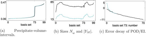
(b) shows furthermore that the number of the magic nodes is roughly higher than the number of POD modes as expected due to the choice of the two stop conditions for the EIM. Also depicted in (c) is the error decay of the POD and EIM. Both errors decay rapidly indicating a strong compressing ability of the high-dimensional model for
. For the basis sets
,
and
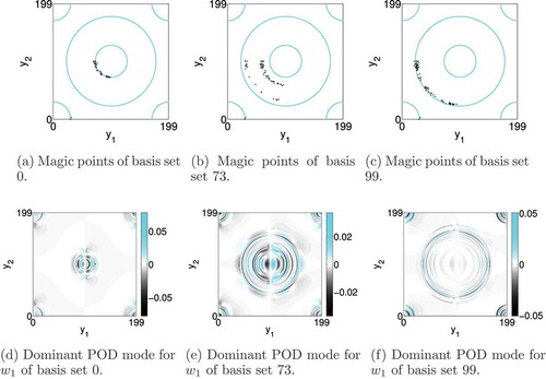
, the distribution of the magic points and the dominant POD mode are illustrated in . For each basis set, the magic points are located in the water domains’ diffuse boundaries of the used snapshots. Therefore, for an increasing index of the basis sets the magic points move from inner regions of the pore-space to outer ones, due to the increasing volume of the precipitates. There are two locations in basis set
, since it handles a large interval of precipitate volumes, and there is a gap between the smaller and the larger ones. The characteristic shapes of the dominant POD modes also travel from inner to outer regions of the pore-space.
Figure 8. Results for setting and the low-dimensional solution
, which consists of
basis sets: (a), (b) and (c) illustrates the distribution of the magic points in the basis sets
,
and
, where the inner circle marks the smallest and the outer one the largest subdomain supporting the precipitate in the snapshots, and the four quarters of a circle indicate the almost unchanged oil phase; (d), (e) and (f) depict the dominant POD mode for
for the corresponding basis sets.
In summary, this subsection showed that the reduced models are capable of reproducing the training data and demonstrated their desired efficiency in comparison to the high-dimensional discretization.
4.3. The settings S2 and S3: the generalization ability of the reduced models
The reduced models of the previous subsection were constructed from snapshots of the setting . In this subsection, the generalization ability of these models is tested for. illustrates high-dimensional results for the settings
and
that differ from
in the parameters tabulated in . The time-interval of
and
is
instead of
, the macroscopic domains are quadratic and also only half the size of
in
and the precipitates with larger volumes are located in the outer subdomain
of
. The initial macroscopic concentration
instead of
in
, the macroscopic function
increases monotonically from
to
in
and to
in
instead of from
to
in
, and the initial radii of the microscopic precipitates are
for
,
for
and
for
in
as well as
for
,
for
and
for
in
. The shape of the time-interval and the macroscopic domain do not influence the microscopic evolution of
and
, but on the other hand the evolution of the macroscopic concentration
certainly does, as well as obviously do the initial radii
of the precipitates.
Figure 9. High-dimensional solutions of the settings and
in the end of the time-interval at
.
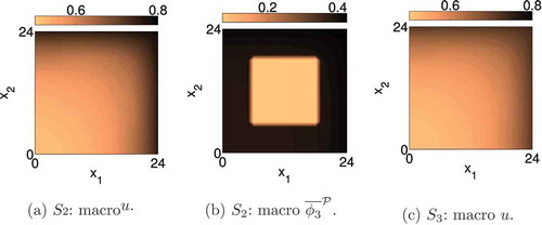
For , shows that the reduced solution converges to the high-dimensional solution for the POD tolerance
tending to zero. In contrast, in case of
the reduced results do not converge to the high-dimensional solution () but instead remain on an acceptable level of accuracy. Since the reduced models were developed from snapshots of
, these observations yield that the high-dimensional solution space for
of
must to be closer to
’s solution space than the one of
, where the initial radius
of the precipitates seems to make the significant difference.
Table 4. Setting S2: the approximations’ accuracy.
Table 5. Setting S3: the approximations’ accuracy.
To sum up, the constructed efficient reduced two-scale models produce accurate results for a wide range of settings as long as the settings’ solution spaces for are close enough to the training setting’s one.
5. Conclusion and outlook
This article presented a model reduction procedure for a complex time-dependent two-scale model for precipitation in porous media. The model used advanced model reduction tools, in particular POD for state compression, EIM for the parameter dependency and multiple basis sets for treating the difficult problem of evolving phase boundaries. Numerical results comparing the overall high- and low-dimensional solutions of the two-scale model demonstrate that the reduced model is on the one hand capable of reproducing the high-dimensional training data and on the other hand can approximate solutions of generalized parameter settings – both extremely efficiently.
This study clearly put a methodological and numerical focus. Future work may address rigorous error analysis for the presented model reduction. The resulting reduced model avoids any operations of complexity (or even any operations of superlinear complexity) during its online phase. But still it requires operations linear in H, which may be prohibitive in more refined space discretizations or in three-space dimensions. Therefore, a further step could consist in providing a reduced scheme that approximates all fields on the microscale (i.e. spaces for all unknowns) and avoids any operation of complexity H. However, the acquired efficiency already fulfils our current requirements.
Acknowledgements
The authors would like to thank the Baden-Württemberg Stiftung gGmbH for funding this project. Also, we thank the German Research Foundation (DFG) for financial support within the Cluster of Excellence in Simulation Technology: [Grant Number EXC 310/1] and within the International Research Training Group ‘Nonlinearities and upscaling in porous media’ [NUPUS, IRTG 1398] at the University of Stuttgart.
Disclosure statement
No potential conflict of interest was reported by the authors.
Additional information
Funding
Notes
1. We give a short motivation for this choice of snapshots for EI: Equation (15) is equivalent to the root finding problem . Standard training snapshots
are always zero, hence carry no suitable information. Motivated by the Newton fixpoint iteration
we realize that for good approximation of this system (and thus good approximation of the fixpoint, i.e. the root) it seems reasonable to collect snapshots
for constructing an EI space. In this sense, we are realizing an EI for the linearized root finding problem, which in our case is the original linear problem (15).
References
- M. Redeker, I.S. Pop, and C. Rohde, Upscaling of a tri-phase phase-field model for precipitation in porous media, University of Stuttgart, preprint (2014). Available at http://www.nupus.uni-stuttgart.de/07_Preprints_Publications/Preprints/Preprints-PDFs/Preprint_2014-6.pdf.
- J. Bear, Dynamics of Fluids in Porous Media, Dover Publications, Mineola, NY, 1988.
- U. Hornung (ed.), Homogenization and Porous Media, Springer, New York, 1997.
- G. Caginalp, An analysis of a phase field model of a free boundary, Arch. Ration. Mech. Anal. 92 (1986), pp. 205–245. doi:10.1007/BF00254827
- G. Caginalp and P. Fife, Dynamics of layered interfaces arising from phase boundaries, SIAM J. Appl. Math. 48 (3) (1988), pp. 506–518. doi:10.1137/0148029
- F. Boyer and C. Lapuerta, Study of a three component Cahn-Hilliard flow model, ESAIM Math. Model. Numer. Anal. 40 (4) (2006), pp. 653–687. doi:10.1051/m2an:2006028
- F. Boyer, C. Lapuerta, S. Minjeaud, B. Piar, and M. Quintard, Cahn–Hilliard/Navier–Stokes model for the simulation of three-phase flows, Transp. Porous. Med. 82 (2010), pp. 463–483. doi:10.1007/s11242-009-9408-z
- X. Li, J. Lowengrub, A. Rätz, and A. Voigt, Solving PDEs in complex geometries: a diffuse domain approach, Commun. Math. Sci. 7 (2009), pp. 81–107. doi:10.4310/CMS.2009.v7.n1.a4
- S. Boyaval, Reduced-basis approach for homogenization beyond the periodic setting, Multiscale Model. Simul. 7 (1) (2008), pp. 466–494. doi:10.1137/070688791
- D.J. Knezevic and A.T. Patera, A certified reduced basis method for the Fokker–Planck equation of dilute polymeric fluids: Fene dumbbells in extensional flow, SIAM J. Sci. Comput. 32 (2) (2010), pp. 793–817. doi:10.1137/090759239
- N.C. Nguyen, A multiscale reduced-basis method for parametrized elliptic partial differential equations with multiple scales, J. Comput. Phys. 227 (23) (2008), pp. 9807–9822. doi:10.1016/j.jcp.2008.07.025
- S. Kaulmann, B. Flemisch, B. Haasdonk, K.-A. Lie, and M. Ohlberger, The localized reduced basis multiscale method for two-phase flows in porous media, Int. J. Numer. Methods Eng. (2015). doi:10.1002/nme.4773
- S. Kaulmann, M. Ohlberger, and B. Haasdonk, A new local reduced basis discontinuous Galerkin approach for heterogeneous multiscale problems, C. R. Acad. Sci. Paris Series I 349 (23–24) (2011), pp. 1233–1238. doi:10.1016/j.crma.2011.10.024
- D. Wirtz, N. Karajan, and B. Haasdonk, Surrogate modelling for multiscale models using kernel methods, Int. J. Numer. Methods Eng. 101 (1) (2015), pp. 1–28. doi:10.1002/nme.4767
- M. Redeker and B. Haasdonk, A POD-EIM reduced two-scale model for crystal growth, Adv. Comput. Math. 41 (5) (2015), pp. 987–1013.
- I.T. Jolliffe, Principal Component Analysis, Springer-Verlag, Berlin/Heidelberg, 2002.
- S. Volkwein, Lecture Notes: Proper Orthogonal Decomposition: Theory and Reduced-Order Modelling, University of Constance, Constance, 2013.
- M. Barrault, Y. Maday, N.C. Nguyen, and A.T. Patera, An empirical interpolation method: application to efficient reduced-basis discretization of partial differential equations, C. R. Acad. Sci. Paris Series I 339 (2004), pp. 667–672. doi:10.1016/j.crma.2004.08.006
- M. Grepl, Y. Maday, N. Nguyen, and A. Patera, Efficient reduced-basis treatment of nonaffine and nonlinear partial differential equations, ESAIM Math. Model. Numer. Anal. 41 (3) (2007), pp. 575–605. doi:10.1051/m2an:2007031
- B. Haasdonk, M. Ohlberger, and G. Rozza, A reduced basis method for evolution schemes with parameter-dependent explicit operators, ETNA Elec. Trans. Numer. Anal. 32 (2008), pp. 145–161.
- M. Drohmann, B. Haasdonk, and M. Ohlberger, Reduced basis approximation for nonlinear parametrized evolution equations based on empirical operator interpolation, SIAM J. Sci. Comput. 34 (2) (2012), pp. A937–A969. doi:10.1137/10081157X
- S. Chaturantabut and D.C. Sorensen, Application of POD and DEIM on dimension reduction of non-linear miscible viscous fingering in porous media, Math. Comp. Model. Dyn. 17 (4) (2011), pp. 337–353. doi:10.1080/13873954.2011.547660
- D. Wirtz, D. Sorensen, and B. Haasdonk, A-posteriori error estimation for DEIM reduced nonlinear dynamical systems, SIAM J. Sci. Comput. 36 (2) (2014), pp. A311–A338. doi:10.1137/120899042
- D. Amsallem, M.J. Zahr, and K. Washabaugh, Fast local reduced basis updates for the efficient reduction of nonlinear systems with hyper-reduction, Adv. Comput. Math. 41 (5) (2015), pp. 1187–1230. doi:10.1007/s10444-015-9409-0
- B. Peherstorfer and K. Willcox, Online adaptive model reduction for nonlinear systems via low-rank updates, SIAM J. Sci. Comput. 37 (4) (2015), pp. A2123–A2150. doi:10.1137/140989169
- D. Amsallem, M. Zahr, and C. Farhat, Nonlinear model order reduction based on local reduced-order bases, Int. J. Numer. Methods Eng. 92 (2012), pp. 891–916. doi:10.1002/nme.4371
- J. Eftang, A. Patera, and E. Rønquist, An hp certified reduced basis method for parametrized elliptic partial differential equations, SIAM J. Sci. Comput. 32 (6) (2010), pp. 3170–3200. doi:10.1137/090780122
- J.L. Eftang, D. Knezevic, and A. Patera, An hp certified reduced basis method for parametrized parabolic partial differential equations, Math. Comp. Model. Dyn. 17 (4) (2011), pp. 395–422. doi:10.1080/13873954.2011.547670
- B. Haasdonk, M. Dihlmann, and M. Ohlberger, A training set and multiple basis generation approach for parametrized model reduction based on adaptive grids in parameter space, Math. Comp. Model. Dyn. 17 (2012), pp. 423–442. doi:10.1080/13873954.2011.547674
- B. Peherstorfer, D. Butnaru, K. Willcox, and H. Bungartz, Localized discrete empirical interpolation method, SIAM J. Sci. Comput. 36 (1) (2014), pp. A168–A192. doi:10.1137/130924408
- B. Wieland, Implicit partitioning methods for unknown parameter domains, Adv. Comput. Math. 41 (2015), pp. 1159–1186. doi:10.1007/s10444-015-9404-5
- M. Geuss, H.K. Panzer, T. Wolf, and B. Lohmann, Stability preservation for parametric model order reduction by matrix interpolation, European Control Conference (ECC), Strasbourg, 2014, pp. 1098–1103, June 2014.
- M. Redeker and C. Eck, A fast and accurate adaptive solution strategy for two-scale models with continuous inter-scale dependencies, J. Comput. Phys. 240 (2013), pp. 268–283. doi:10.1016/j.jcp.2012.12.025