An empirical interpolation approach to reduced basis approximations for variational inequalities

ABSTRACT

Variational inequalities (VIs) are pervasive in mathematical modelling of equilibrium and optimization problems in engineering and science. Examples of applications include traffic network equilibrium problems, financial equilibrium, obstacle problems, lubrication phenomena and many others. Since these problems are computationally expensive to solve, we focus here on the development of model order reduction techniques, in particular the reduced basis technique. Reduced basis techniques for the approximation of solutions to elliptic VIs have been developed in the last few years. These methods apply to VIs of the so-called first kind, i.e. problems that can be equivalently described by a minimization of a functional over a convex set. However, these recent approaches are inapplicable to VIs of the so-called second kind, i.e. problems that involve minimization of a functional containing non-differentiable terms. In this article, we evaluate the feasibility of using the reduced basis method (RBM) combined with the empirical interpolation method (EIM) to treat VIs. In the proposed approach, the problem is approximated using a penalty or barrier method, and EIM is then applied to the penalty or barrier term. Numerical examples are presented to assess the performance of the proposed method, in particular the accuracy and computational efficiency of the approximation. Although the numerical examples involve only VIs of the first kind, we also evaluate the feasibility of using the RBM combined with the EIM to treat VIs of the second kind.

KEYWORDS:

• Reduced basis method
• empirical interpolation method
• variational inequalities
• barrier method
• penalty method
• obstacle problem

AMS CLASSIFICATION:

• 65K10
• 65K15

1. Introduction

Many problems in engineering and science can be described as elliptic variational inequalities (VIs). Before addressing such problems in function spaces, we first give the reader a simple example. It is inspired by [1] and addresses a scalar minimization problem.

Let $I:=[a,b]$, $a\le b$ be an interval and f :I → $\mathbb{R}$ be a continuously differentiable function. Since f is continuous, it has a minimum in I. The minimum x is characterized in the following way:

$f^{\prime }(x)=0,\mathrm{i}\mathrm{f}a<x<b,$

$f^{\prime }(x)\ge 0,\mathrm{i}\mathrm{f}x=a,$

$f^{\prime }(x)\le 0,\mathrm{i}\mathrm{f}x=b.$

The last characterization can be reformulated into a single statement

$f^{\prime }(x)\cdot (y-x)\ge 0\mathrm{\forall }\hspace{0.17em}y\in I,$

which is a VI-problem in $\mathbb{R}$. In the following, we generalize the problem to the Banach space setting. There the minimum of a functional does not lie in an interval but in a convex set.

In particular, we consider ‘elliptic VI-problems of the first kind’. Such problems are defined as a minimization of a sum of a bilinear and linear functional over a convex set X (see, e.g., [2]): $arg\underset{v\in X}{min}\frac{1}{2}a(v,v)-f(v)$, or equivalently $a(u,v-u)-f(v-u)\ge 0\mathrm{\forall }\hspace{0.17em}v\in X$. This class of problems includes, among other problems, obstacle problems, lubrication phenomena and two-dimensional flows of perfect fluids or wake problems.

In this article, we focus on minimizing functionals with a bilinear and (non)linear part, such as obstacle-like problems. The problem’s underlying physics is described by parameters: material, geometry and boundary properties. For a fixed parameter, the solution procedure for VIs, in practice, often relies on Lagrange-, barrier- or penalty-based methods (see, e.g., [3]) and is often costly. Especially, in real-time (e.g. parameter-estimation) and many-query (e.g. design optimization) contexts, it is necessary to find faster ways to solve VIs for many parameters. One key ingredient is exploring the parameter-induced solution-manifold and trying to resolve it with only a few functions.

The reduced basis method (RBM) was successfully applied in [4,5], and [6] to the Lagrange-based approach for VIs of the first kind with bilinear and linear functional parts only. In [5] the computation of surrogate solutions, and a posteriori error bounds with a partial offline-online computational decomposition are presented. The idea of such a decomposition is to pre-compute offline costly terms in advance and then, online, rapidly – without high-dimensional computations – compute a surrogate solution and its error estimator.

In this paper we focus primarily on solving VIs in which the ‘cost’ function is a sum of a bilinear and a nonlinear functional. We investigate the feasibility of solving these VIs by applying the empirical interpolation method (EIM) to the barrier- and penalty-based formulations. Although the problems considered here involve differentiable nonlinear functions, our ultimate goal is to evaluate the proposed method’s practicability for VIs of the second kind, i.e. VIs involving non-differentiable functionals. VIs of the second kind play an important role in friction and contact (see, e.g., [7]) and are even more difficult to handle.

We focus on the development of rapidly convergent reduced basis surrogates and associated a posteriori error estimators, following three steps. First, we eliminate the Lagrange multiplier by applying the barrier or penalty method. This adds a non-linear term to the functional. Second, we apply EIM to the latter non-linear term, in order to evaluate it rapidly yet accurately. Third, we reduce the dimension of the problem through a Galerkin projection onto a low-dimensional reduced basis space and an efficient evaluation of the non-linearity by EIM. Using these three steps, we rapidly compute a surrogate. Moreover, this surrogate is used to evaluate a non-rigorous a posteriori error estimator. More precisely, this estimator approximates the error but does not bound it rigorously.

We start with the general problem setting. Let $\mathrm{\Omega }\subset {\mathbb{R}}^d$ be the physical domain and $\mu \in \mathcal{P}\subset {\mathbb{R}}^p$ represent parameters. The VI is described by a minimization problem on a convex subset X(μ) of a separable Hilbert space V. Find $u\in X(\mu )$, such that

(1) $u=arg\underset{v\in X(\mu )}{min}J(v),J(v):=\frac{1}{2}a(v,v)-f(v).$(1)

We assume that a(∙,∙) is a symmetric, continuous and coercive bilinear form. Furthermore, we distinguish two cases for a bounded functional f(∙): In Section 2, we consider a linear f(∙), whereas in Section 4, we consider an example with a non-linear f(∙). Here, for simplicity, we only allow the parameter μ to influence the admissible space X(μ) by the means of $u(x)\ge h(x;\mu )$, where $h(\cdot ;\mu )\in C(\bar{\mathrm{\Omega }})$. However, our approach is easily extendable to parameter-dependent a(∙,∙) and f(∙). Note that here $u\in C(\bar{\mathrm{\Omega }})$ since for $X(\mu )\subset H^1(\mathrm{\Omega })=V$ and $\mathrm{\Omega }\subset {\mathbb{R}}^1$, the Sobolev embedding theorem implies $u\in H^1(\mathrm{\Omega })\subset C(\bar{\mathrm{\Omega }})$ (see, e.g., [2]). Since u is continuous, the restriction $u(x)\ge h(x;\mu )$ is well defined. However, for higher spatial dimensions, the continuity of u is not ensured, but we can define an embedding $H^1(\mathrm{\Omega })\to L_2(\mathrm{\Omega })$ and so consider the order relation ≥ in the weak L₂-sense.

We state the main contributions of this article:

• We investigate the feasibility of solving (non-linear) VIs by applying the EIM to the barrier- and penalty-based formulations.

• We study the quality of error estimators provided by the EIM-RB reduction.

• We successfully apply our methods to VIs including convex differentiable terms, such as $|u{|}^3$.

In Section 2, we introduce two solution procedures, a barrier method and an exponential penalty method (exp-penalty method), and derive the equivalence of a VI and a non-linear elliptic equation. In Section 3, we (i) briefly introduce the application of EIM and RBM to non-linear elliptic equations and (ii) derive two a posteriori error estimators. In Section 4, we present numerical results for an one-dimensional (1D) model problem with an obstacle-type constraint.

2. Barrier method and exponential penalty method

We first introduce a regularization with a barrier method with an obstacle-like, parameter-dependent constraint $u(x)\ge h(x;\mu )$. The idea of the barrier methods is to substitute the constraint by a smooth and monotone so-called barrier functional that raises to infinity if the solution approaches the constraint. Therefore, the constraint is incorporated in the barrier functional $B(u;\mu )={\int }_{\mathrm{\Omega }}-ln(u(x)-h(x;\mu ))\hspace{0.17em}\mathrm{d}\mathrm{\Omega }$, where $u(x)>h(x;\mu )$ is necessary for the well-posedness. Overall, the new functional $J_B(u;\mu ,\nu ):=J(u)+\nu \cdot B(u;\mu )$ is still convex in u for all $\nu$ and therefore a minimizer $u(\cdot ;\mu ,\nu ):=arg\underset{v\in V}{min}{J}_B(v;\mu ,\nu )$ exists.

The discretized problems of $J_B(u;\mu ,\nu )$ and Equation (1) can be treated by non-linear convex programming, for which the authors of [8] show convergence for a decreasing parameter $\nu$. More precisely, the solution of the discretized problem $arg\underset{v\in V}{min}{J}_B(v;\mu ,\nu )$ converges to the solution of the discretized problem (Equation (1)).

Further, we characterize the minimizer u(∙; μ, $\nu$) for a linear f(∙) by the first order necessary (here, also sufficient) condition:

(2) $J^{\prime }(u)[v]+\nu \cdot B^{\prime }(u;\mu )[v]=a(u,v)-f(v)-\nu \cdot {\int }_{\mathrm{\Omega }}\frac{v(x)}{u(x)-h(x;\mu )}\mathrm{d}\mathrm{\Omega }=0.$(2)

In order to approach a solution of Equation (1), we solve Equation (2) for a sequence of decreasing homotopy parameters $\nu$ and follow a continuation procedure combined with Newton’s method. More precisely, we start to solve Equation (2) with the Newton’s method for a relatively large $\nu$₀ ≈ 0.2. This $\nu$₀ is chosen such that the Newton’s method converges in a few steps and u($\nu$₀) is relatively close to the unconstrained problem of Equation (1). Once the Newton’s method has converged, we decrease $\nu$ by a fixed factor γ (e.g. we take γ = 2/3) such that $\nu$₁ = γ · $\nu$₀. Then, we solve Equation (2) for u($\nu$₁) using u($\nu$₀) as the initial guess in the Newton’s method. We eventually stop when we obtain the solution of Equation (2) for the final homotopy parameter $\nu$_final = 1E – 3. The convergence of the Newton’s method for all $\nu$ > 0 is ensured for the discretized setting (see Chapter 11.2 in [8]). The construction of the $\nu$-sequence, here, is based on the following observations: (i) for $\nu$₀ the Newton’s method converges in a few steps, (ii) the factor γ = 2/3 was sufficient to provide on the one side a good initial guesses for solving Equation (2) for the next ${\nu }_{i+1}$ and on the other side not to include too many intermediate $u(\nu {\hspace{0.17em}}_i)$-solutions and (iii) we choose ${\nu }_{\mathrm{f}\mathrm{i}\mathrm{n}\mathrm{a}\mathrm{l}}$ such that the regularization error caused by the $\nu$-sequence is close to the discretization error (see Section 4). In our model problems, we did not encounter any convergence problems. 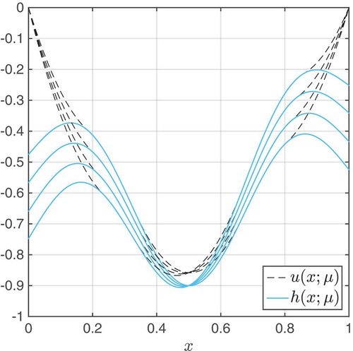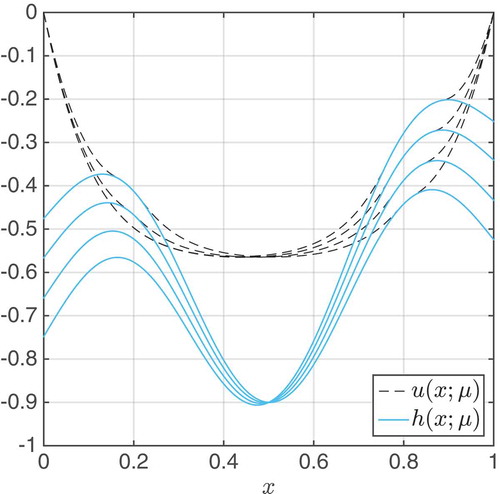For a detailed discussion on the initial parameter $\nu$₀ and the construction of the $\nu$-array, we refer to Chapter 11.3.1 in [8]. In Figure 1, we anticipate the numerical example in Section 4 and show solutions for the obstacle problem.

Figure 1. Solutions u(x; μ) and the corresponding obstacles h(x; μ) of the first numerical example in Section 4.

Second, we introduce a penalty approach. The standard penalty method with a quadratic penalization functional is widely used and has been analysed (see, e.g., [9,7]). Since the quadratic penalty term is only once-differentiable, we introduce a smoother penalization with an exponential term. This penalization has been already proposed for non-linear convex programming in $\mathbb{R}$ⁿ, (see, e.g., [10,11]). In this work, we extend the exp-penalty method to the function space setting.

Analogously to the barrier method, we define an additional penalizing term $E(u;\mu ,\nu ):=\nu \int (exp(1/\nu \cdot (h(x;\mu )-u(x))\hspace{0.17em})-1)\mathrm{d}\mathrm{\Omega }$ with $\nu$ → 0. The term E(u; μ, $\nu$) becomes larger, if u violates h(μ). Since for all fixed $\nu$ > 0 the term E(u; μ, $\nu$) is convex, we can identify a $\nu$-dependent minimization problem: find u($\nu$) minimizing $J(u)+E(u;\mu ,\nu )\mathrm{\forall }u\in V$. Again, we characterize u($\nu$) by the first-order optimality condition $J^{\prime }(u)[v]+E^{\prime }(u;\mu ,\nu )[v]=a(u,v)-f(v)-{\int }_{\mathrm{\Omega }}exp(1/\nu \cdot (h(x;\mu )-u(x))\hspace{0.17em})v(x)\mathrm{d}\mathrm{\Omega }=0\mathrm{\forall }v\in V.$ We then solve this non-linear elliptic equation for a fixed $\nu$ by using a damped Newton’s method and a decreasing $\nu$-sequence in a homotopy. In practice, we use the same sequence as in the barrier method.

Based on the convergence results of the exp-penalty method for discrete spaces in [10,11], we carry out finite-dimensional calculations in Section 4.

3. Empirical interpolation method and reduced basis method

In this section, we introduce well-known reduction techniques and combine them to explore one way to (i) rapidly compute accurate approximations to parametrized VIs and (ii) explore the parameter-induced solution manifold.

We will focus on the barrier method only in this section; all the results can be directly transferred to the exp-penalty method. We start by introducing a discrete and computable framework for the barrier method. Let Ω_h be a discrete domain space and V_h a high fidelity finite element method-space that is fine enough to resolve the parameter-dependent solution sufficiently well. In this article, we use P₁ piecewise linear hat basis functions. In order to reduce the computational cost, we first, introduce EIM to reduce the complexity of the non-linear term in Equation (2) and, second, apply RBM to reduce the complexity of the linear and bilinear terms. Based on these two steps, we derive a reduced Newton’s method and an error indicator that estimates the quality of the reduced solution.

3.1. EIM

The formulation of the barrier method in Equation (2) involves a μ-dependent non-linear term $\nu \cdot \frac{1}{u-h(\mu )}=:g(u,x;\mu )$, which we need to efficiently approximate for a fixed, here, final $\nu ={\nu }_{\mathrm{f}\mathrm{i}\mathrm{n}\mathrm{a}\mathrm{l}}$. EIM provides such an approximation by a coefficient function approximation $g_M(x;\mu )$ with $g_M(x;\mu )\approx g(u(x;\mu ),x;\mu )$. We define $g_M(x;\mu )$ in Algorithm 1 and restate major results from [12] and [13].

EIM is based on a greedy approach to successively construct so-called interpolation points $T_M=\{x_1,\dots ,x_M\}\subset {\mathrm{\Omega }}_h$ and a sample set $S_M\equiv \{{\mu }_1,\dots ,{\mu }_M\}\subset \mathcal{P}$ with the associated reduced space $W_M=\mathrm{s}\mathrm{p}\mathrm{a}\mathrm{n}\{q_1\in V_h,\dots ,q_M\in V_h\}$. The approximation $g_M$ lies in the latter space $g_M\in W_M$. The EIM approach consists of the following three steps:

First, we choose a maximal dimension of the space W_M : $M_{max}\ge 2$, and define a finite parameter training set ${\mathrm{\Xi }}_{\mathrm{t}\mathrm{r}\mathrm{a}\mathrm{i}\mathrm{n}}^{\mathrm{E}\mathrm{I}\mathrm{M}}\subset \mathcal{P}$ for which we compute u(μ) and $g(u(x;\mu ),x;\mu )$ for all $\mu \in {\mathrm{\Xi }}_{\mathrm{t}\mathrm{r}\mathrm{a}\mathrm{i}\mathrm{n}}^{\mathrm{E}\mathrm{I}\mathrm{M}}.$

Second, we compute the first basis function of the coefficient function approximation by the following four ingredients: (i) choose one parameter ${\mu }_1\in {\mathrm{\Xi }}_{\mathrm{t}\mathrm{r}\mathrm{a}\mathrm{i}\mathrm{n}}^{\mathrm{E}\mathrm{I}\mathrm{M}}$, (ii) set ${\xi }_1\equiv g(u(x;{\mu }_1),x;{\mu }_1)$, (iii) determine the first interpolation point by $x_1=arg{max}_{x\in {\mathrm{\Omega }}_h}|{\xi }_1(x)|$ and (iv) set the first basis function of W_M as $q_1={\xi }_1(x)/{\xi }_1(x_1)$.

Third, we perform Algorithm 1 that uses data from M previous steps to generate data for M + 1.

Algorithm 1

EIM induction

1. for $M\in \{1,\dots ,M_{max}\}$ do

2. define $B_{ij}^M=q_j(x_i)$ for $1\le j\le i\le M$ ; else $B_{ij}^M=0$

3. solve ${\sum }_{j=1}^M{B}_{ij}^M{\phi }_{M\hspace{0.17em}j}(\mu )=g(u(x_i;\mu ),x_i;\mu ),1\le i\le M$ for ${\phi }_M(\mu )$ $\mathrm{\forall }\mu \in {\mathrm{\Xi }}_{\mathrm{t}\mathrm{r}\mathrm{a}\mathrm{i}\mathrm{n}}^{\mathrm{E}\mathrm{I}\mathrm{M}}$

4. compute $g_M(x;\mu )={\sum }_{m=1}^M{\phi }_{M\hspace{0.17em}m}(\mu )q_m(x)$ $\mathrm{\forall }\mu \in {\mathrm{\Xi }}_{\mathrm{t}\mathrm{r}\mathrm{a}\mathrm{i}\mathrm{n}}^{\mathrm{E}\mathrm{I}\mathrm{M}}$ and compute the

5. interpolation error ${\epsilon }_M(\mu )=\parallel g(u(\cdot ;\mu ),\cdot ;\mu )-g_M(\cdot ;\mu ){\parallel }_{L^{\mathrm{\infty }}(\mathrm{\Omega })},$ $\mu \in {\Xi }_{\text{train}}^{\text{EIM}}$

6. determine ${\mu }_{M+1}\equiv arg{max}_{\mu \in {\mathrm{\Xi }}_{\mathrm{t}\mathrm{r}\mathrm{a}\mathrm{i}\mathrm{n}}^{\mathrm{E}\mathrm{I}\mathrm{M}}}{\epsilon }_M(\mu )$ and $x_{M+1}\equiv arg{max}_{x\in {\mathrm{\Omega }}_h}{\epsilon }_M(x;{\mu }_{M+1})$

7. set $r_{M+1}(x)=g(u(\cdot ;{\mu }_{M+1}),\cdot ;{\mu }_{M+1})-g_M(\cdot ;{\mu }_{M+1})$ and $q_{M+1}(x)=r_{M+1}(x)/r_{M+1}(x_{M+1})$

8. define $T_{M+1}=T_M\cup x_{M+1}$, $S_{M+1}=S_M\cup {\mu }_{M+1}$ and $W_{M+1}=W_M\cup q_{M+1}$

9. end for

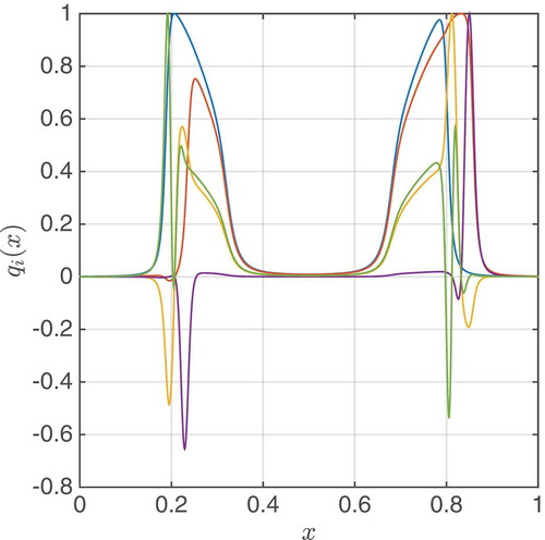
Note that in Algorithm 1, the matrix B^M is lower triangular with unity diagonal and hence invertible. Further, using the EIM approach, we depict the first five basis functions of W_M for the first numerical example in Figure 2. It is worth mentioning that if the functional f(∙) has non-linear parts, they can be simply included in the functional g(∙) and also treated by the proposed EIM reduction. We can thus assume in the subsequent sections that f(∙) is linear. We now turn to the RB method.

Figure 2. The first five basis vectors forming g_M’s space W_M in the numerical example for the barrier method in Section 4. The basis $\{q_i{\}}_{i=1}^5$ is constructed by EIM.

3.2. RBM

It has been shown that RBM efficiently reduces the complexity for many parametrized problems, such as elliptic [14], transport dominated [15], parabolic [16] and even hyperbolic problems [17,18].

Based on the RBM results for elliptic problems, we give the following reduced basis setting. We introduce a nested sample $S_N^u:=\{{\mu }_1^u,...,{\mu }_N^u\}\subset \mathcal{P},1\le N\le N_{max}\in \mathbb{N}$; see later for construction of samples obtained by the greedy approach. Further, we define the associated nested reduced basis space $W_N^u:=\{{\zeta }_i;1\le i\le N\},1\le N\le N_{\mathrm{m}\mathrm{a}\mathrm{x}}$, where ${\zeta }_i\equiv u({\mu }_i^u)$ is the solution of the barrier method for the final and smallest homotopy parameter $\nu ={\nu }_{\mathrm{f}\mathrm{i}\mathrm{n}\mathrm{a}\mathrm{l}}$. Further, we orthonormalize ${\zeta }_i;1\le i\le N_{\mathrm{m}\mathrm{a}\mathrm{x}}$ with respect to the inner product $(\cdot ,\cdot {)}_V=:a(\cdot ,\cdot )$ such that the Newton’s Jacobian matrix (to be defined in Section 3.5) is better conditioned. Subsequently, we apply a Galerkin projection for the non-linear elliptic Equation (2), for the final homotopy parameter $\nu$_final, onto the space $W_N^u$ and search for a surrogate solution $u_N(\mu )\in W_N^u$ for any $\mu \in \mathcal{P}$. The resulting non-linear reduced problem is given by $a(u_N(\mu ),v)-f(v)-{\int }_{\mathrm{\Omega }}g(u_N(x;\mu ),x;\mu )v\mathrm{d}\mathrm{\Omega }=0,v\in W_N^u$. By considering the representation of $u_N(\mu )={\sum }_{i=1}^N{u}_{Ni}(\mu )\cdot {\zeta }_i\in W_N^u$, we get a smaller algebraic system ${\sum }_{j=1}^{N}a({\zeta }_i,{\zeta }_j)u_{Nj}(\mu )-f({\zeta }_i)-{\int }_{\mathrm{\Omega }}g(u_N(x;\mu ),x;\mu )\cdot {\zeta }_i(x)\mathrm{d}\mathrm{\Omega }=0,1\le i\le N$. We see immediately that the latter system cannot be solved online efficiently, since $g(u_N(x;\mu ),x;\mu )$ is non-linear in u_N and therefore cannot be decomposed in the offline stage. Consequently, we apply the EIM-approximation to the latter term, which leads to a reduced problem with the unknown $u_{NM}(\mu )\in {\mathbb{R}}^N$:

(3) $\sum _{j=1}^{N}a({\zeta }_i,{\zeta }_j)u_{NMj}(\mu )-f({\zeta }_i)-{\int }_{\mathrm{\Omega }}{g}_M(x;\mu )\cdot {\zeta }_i(x)\mathrm{d}\mathrm{\Omega }=0,1\le i\le N.$(3)

We can rapidly access ${\int }_{\mathrm{\Omega }}{g}_M(x;\mu )\cdot {\zeta }_i(x)\mathrm{d}\mathrm{\Omega }={\sum }_{m=1}^M{\phi }_{Mm}(\mu ){\int }_{\mathrm{\Omega }}{\zeta }_i{q}_m\mathrm{d}\mathrm{\Omega }$, which completes the online–offline decomposition. Through this decomposition, we can now solve Equation (3) and obtain a surrogate $u_{NM}(x;\mu )$ for the original problem (Equation (1)). Note that here we do not consider $\nu$ as a parameter for the RBM, but include implicitly the final homotopy parameter $\nu$_final in g_M, in Equation (3).

3.3. Greedy procedure

In this subsection, the sample set $S_N^u$ and the corresponding RB-space $W_N^u$ are constructed for the final homotopy parameter $\nu$_final in four steps: First, let ${\mathrm{\Xi }}_{\mathrm{t}\mathrm{r}\mathrm{a}\mathrm{i}\mathrm{n}}\subset \mathcal{P}$ be a training set, which is usually larger than ${\mathrm{\Xi }}_{\mathrm{t}\mathrm{r}\mathrm{a}\mathrm{i}\mathrm{n}}^{\mathrm{E}\mathrm{I}\mathrm{M}}$, since from our experience we need more training parameters to sufficiently explore the μ-induced solution manifold. If $S_N^u=\mathrm{\varnothing }$, then choose an initial parameter ${\mu }_1\in {\mathrm{\Xi }}_{\mathrm{t}\mathrm{r}\mathrm{a}\mathrm{i}\mathrm{n}}$ and set μ* = μ₁. Second, add μ* into $S_N^u$ and the corresponding solution u(·; μ*) into $W_N^u$. Third, compute with M = M_max for all $\mu \in {\mathrm{\Xi }}_{\mathrm{t}\mathrm{r}\mathrm{a}\mathrm{i}\mathrm{n}}$ the surrogate $u_{NM}(\cdot ;\mu )\in W_N^u$ and its approximate relative error estimator $\parallel u(\mu )-u_{NM}(\mu ){\parallel }_V/\parallel u_{NM}(\mu ){\parallel }_V\lesssim {\epsilon }_{\text{est}}\parallel u_{NM}(\mu ){\parallel }_V$. The derivation of $u_{NM}(\cdot ;\mu )$ and $\epsilon$_est is introduced in the following Sections 3.4 and 3.5. Fourth and finally, having $\epsilon$_est, we determine the parameter μ* with the largest $\epsilon$_est to be added into $S_N^u$.

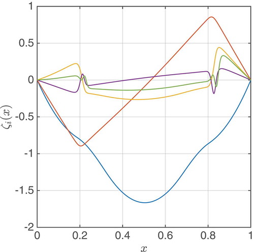
The second, third and fourth steps are repeated until the maximal estimator falls below a tolerance, or a maximal number of reduced basis functions N_max is reached; for a detailed description of the greedy method, see, e.g., [19]. Using the greedy approach, we depict the first five basis function of $W_N^u$ for the first numerical example in Figure 3.

Figure 3. First five basis vectors forming the reduced basis space $W_N^u$ in the numerical example for the barrier method in Section 4. The basis $\{{\zeta }_i{\}}_{i=1}^5$ is constructed by greedy procedure based on the a posteriori error estimator (only the residual part $\epsilon$_NM).

It is worth mentioning that in Figure 2, we see, in the transition area between non-contact and contact, steep gradients. These gradients are hard to approximate for the EIM. The gradients become even steeper for smaller $\nu$_final such that an inaccurate g_M causes inaccurate approximations for u (see Figures 7 and 8).

Figure 4. Relative convergence of barrier/exp-penalty solutions to the reference solution, depending on the homotopy parameter $\nu$, measured in V-norm.

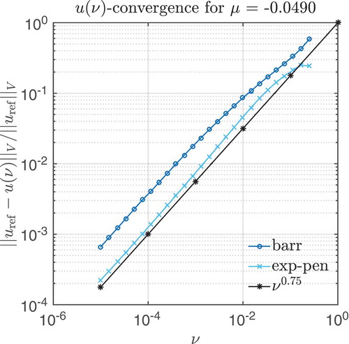
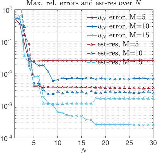
Figure 5. Barrier method: maximal relative error and estimator decay (only residual part) for different N, M values.

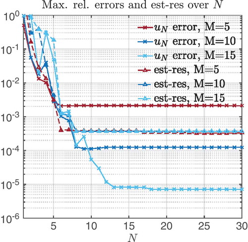
Figure 6. Exp-penalty method: maximal relative error and estimator decay (only residual part) for different N, M values.

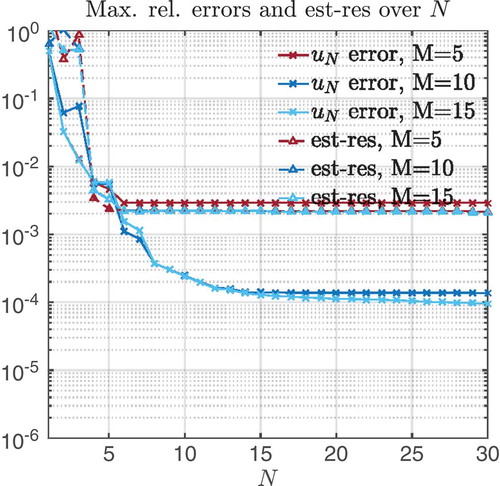
Figure 7. Barrier method: Numerical instabilities for the case when the homotopy parameter is very small ($\nu$_final = 1E – 4). Maximal relative error and estimator decay (only residual part) for different M, N values.

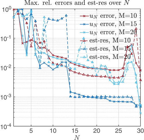
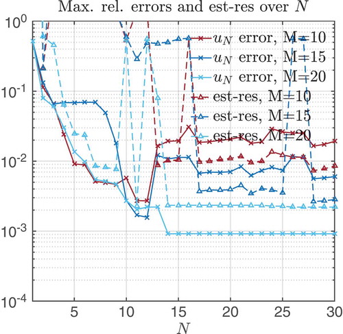
Figure 8. Exp-penalty method: Numerical instabilities the case when the homotopy parameter is very small ($\nu$_final = 1E – 4). Maximal relative error and estimator decay (only residual part) for different M, N values.

In the next part of this section, we give the formulation of the a posteriori error estimator and the explicit construction of Newton’s method in the reduced setting.

3.4. A posteriori error estimator

In order to derive an error estimator, we define the residual term $R_N(v;\mu )$ $=f(v)-a(u_{NM}(x;\mu ),v)+{\int }_{\mathrm{\Omega }}{g}_M(x;\mu )\cdot v(x)\mathrm{d}\mathrm{\Omega }\mathrm{\forall }v\in V_h$. Then we define three auxiliary terms that are used in the estimator derivation: (i) ${\epsilon }_{NM}(\mu ):={sup}_{v\in V_h}{R}_N(v;\mu )/||v|{|}_V$, (ii) ${\vartheta }_M^q:={sup}_{v\in V_h}{\int }_{\mathrm{\Omega }}{q}_{M+1}\cdot v\mathrm{d}\mathrm{\Omega }/||v|{|}_V$ and (iii) ${\hat{\epsilon }}_M(\mu ):=|g(u_{MN}(x_{M+1};\mu ),x_{M+1};\mu )-g_M(x_{M+1};\mu )|$, where $M+1\le M_{\mathrm{m}\mathrm{a}\mathrm{x}}$. We go back to Equation (2), use its full solution u(μ) and conclude

(4) $R_N(v;\mu )=a(u-u_{NM},v)-{\int }_{\mathrm{\Omega }}(g(u,x;\mu )-g_M(x;\mu ))\cdot v\mathrm{d}\mathrm{\Omega },$(4)

(5) $=a(u-u_{NM},v)-{\int }_{\mathrm{\Omega }}(g(u,x;\mu )-g(u_{NM},x;\mu )$(5)

$+g(u_{NM},x;\mu )-g_M(x;\mu ))\cdot v\mathrm{d}\mathrm{\Omega }\mathrm{\forall }v\in V_h.$

Note that $g(u,x;\mu )=\nu \cdot \frac{1}{u-h(\mu )}$ is continuous and monotonically decreasing in u. From that we infer that $\delta (x):=-(g(u,x;\mu )-g(u_{NM},x;\mu ))\cdot (u-u_{NM})\ge 0$ and therefore $\mathcal{A}:={\int }_{\mathrm{\Omega }}\delta (x)\mathrm{d}\mathrm{\Omega }\ge 0$. Next we substitute $\nu$ in Equations (4) and (5) with $e:=u-u_{NM}$ and conclude $a(e,e)+\mathcal{A}=R_N(e;\mu )+{\int }_{\mathrm{\Omega }}(g(u_{NM},x;\mu )-g_M(x;\mu ))\cdot e\mathrm{d}\mathrm{\Omega }$.

At this point, we already derive the first error estimator by neglecting ${\int }_{\mathrm{\Omega }}(g(u_{NM},x;\mu )-g_M(x;\mu ))\cdot e\mathrm{d}\mathrm{\Omega }$. Using (i) $\mathcal{A}\ge 0$ and (ii) $\alpha ||e|{|}_V^2\le a(e,e)$, where α is the coercivity constant of a(∙,∙), we conclude

(6) $||e|{|}_V\lesssim {\epsilon }_{NM}\frac{1}{\alpha }=\underset{v\in V_h}{sup}\frac{R_N(v;\mu )}{||v|{|}_V}\frac{1}{\alpha }.$(6)

In Section 4, we illustrate in the numerical examples that this term is already a good indicator for the error. However, for completeness, we go one step back and consider the neglected term ${\int }_{\mathrm{\Omega }}(g(u_{NM},x;\mu )-g_M(x;\mu ))\cdot e\mathrm{d}\mathrm{\Omega }$. In order to estimate that term we use a special property of EIM: If M + 1 ≤ M_max and $g(u_{NM},x;\mu )\in W_{M+1}$, then $g(u_{NM},x;\mu )-g_M(x;\mu )=\pm {\hat{\epsilon }}_M\cdot q_{M+1}$ (see, e.g., in [12]). Of course, this condition $g(u_{NM},x;\mu )\in W_{M+1}$ is generally not satisfied. Therefore, we make a common EIM assumption that $g(u_{NM},x;\mu )-g_M(x;\mu )\approx \pm {\hat{\epsilon }}_M\cdot q_{M+1}$. Thus, we deduce $\underset{\Omega }{{\displaystyle \int }}(g(u_{NM},x;\mu )-g_M(x;\mu ))\cdot e\text{d}\Omega \lesssim {}_2\widehat{\epsilon }{}_M(\mu )\cdot {\vartheta }_M^q\cdot |\left|e\right|{|}_V$. We infer from $\mathcal{A}$ ≥ 0 and coercivity of a(∙,∙) that

(7) $||e|{|}_V\hspace{0.17em}\lesssim ({\epsilon }_{NM}+{\hat{\epsilon }}_M\cdot {\vartheta }_M^q)/\alpha .$(7)

Here, α = 1, since we did not include any μ dependence for a(∙,∙) and defined (∙,∙)_V = a(∙,∙). If a(∙,∙;μ) is ‘parametrically coercive’, the simple ‘min-θ’ approach can be applied to determine α (see [14]). For even more general bilinear, and even non-symmetric forms, the Successive Constraint Method provides an α (see [14]).

3.5. Reduced Newton’s method

We solved the full problem (Equation (2)) by a continuation procedure with the Newton’s method. We apply exactly the same approach with the same $\nu$-sequence also for the reduced problem (Equation (3)) for $\nu$_final. For the Newton’s method, we need the following two ingredients: first, the reduced Equation (3), which we drive close to zero, and second, the gradient of Equation (3).

Let $u_{NM}\in W_N^u$ be an initial guess, where – except for the first homotopy solution $u_{NM}({\nu }_0)$ – the initialization is given by $u_{NM}({\nu }_{\mathrm{p}\mathrm{r}\mathrm{e}\mathrm{v}\mathrm{i}\mathrm{o}\mathrm{u}\mathrm{s}})$. We denote the representation $u_{NM}=Z\cdot {\underset{\_}{u}}_{NM}$, where $Z=({\zeta }_1,...,{\zeta }_N)\in {\mathbb{R}}^{\mathcal{N}\times N}$ stores the RB vectors and ${\underset{}{\underset{\_}{u}}}_{NM}\in {\mathbb{R}}^N$ is the coefficient vector. Using that representation, we define three algebraic parts: (i) a matrix $A_{N_{i,j}}:=a({\zeta }_i,{\zeta }_j)$, (ii) a vector $F_{N_i}:=f({\zeta }_i)$ and (iii) determine $g(u_{NM},x;\mu )$ at the interpolation points $x_m,1\le m\le M$ and store the values in $g_{\mathrm{i}\mathrm{n}\mathrm{t}}(u_{NM})\in {\mathbb{R}}^M$. In order to evaluate $g_{\mathrm{i}\mathrm{n}\mathrm{t}}(u_{NM})$, we evaluate the basis ζ_i at the x_m and store them in $Z_M\in {\mathbb{R}}^{N\times M}$. Then, we define $g_{\mathrm{i}\mathrm{n}\mathrm{t}}(u_{NM}{)}_m:=g(Z_{M_m}{\underset{\_}{u}}_{NM},x_m;\mu )$. Using the definition of $g_M(x;\mu )$, we derive a new representation of the last term of Equation (3)

${\int }_{\mathrm{\Omega }}{g}_M(x;\mu )\cdot {\zeta }_i(x)\mathrm{d}\mathrm{\Omega }=\sum _{m=1}^M{\int }_{\mathrm{\Omega }}{\left({B^M}^{-1}\cdot g_{\mathrm{i}\mathrm{n}\mathrm{t}}(u_{NM})\right)}_m{q}_m(x)\cdot {\zeta }_i(x)\mathrm{d}\mathrm{\Omega }.$

We define two matrices, $C_{i,m}:={\displaystyle {\int }_{{\hspace{0.17em}}_{\Omega }}{q}_m\cdot {\zeta }_i\text{d}\Omega ,C\in {ℝ}^{N\times M}}$ and $D:=C\cdot {B^M}^{-1}\in {\mathbb{R}}^{N\times M}$, and thus rewrite Equation (3) algebraically into

$A_N\cdot {\underset{\_}{u}}_{NM}-F_N-D\cdot g_{\mathrm{i}\mathrm{n}\mathrm{t}}(u_{NM})=0.$

For the gradient of the last expression, we take derivatives of Equation (3) with respect to the unknown u_NM. This results in the following expression of the gradient $A_N+D\cdot \mathrm{d}\mathrm{i}\mathrm{a}\mathrm{g}(g_{\mathrm{i}\mathrm{n}\mathrm{t}}(u_{NM}))\cdot Z_M\in {\mathbb{R}}^{N\times N},$ where diag(vector) is a matrix with the vector’s entries on the diagonal.

Having now the evaluation of Equation (3) and its gradient, we state the Newton’s iteration: (i) start with a guess u_NM and (ii) compute δu_NM by solving:

$\left(A_N+D\cdot \mathrm{d}\mathrm{i}\mathrm{a}\mathrm{g}(g_{\mathrm{i}\mathrm{n}\mathrm{t}}(u_{NM}))\cdot Z_M\right)\delta {\underset{\_}{u}}_{NM}=A_N\cdot {\underset{\_}{u}}_{NM}-F_N-D\cdot g_{\mathrm{i}\mathrm{n}\mathrm{t}}(u_{NM}),$

(iii) update ${\underset{\_}{u}}_{NM}={\underset{\_}{u}}_{NM}-\kappa \delta {\underset{\_}{u}}_{NM}$, where $\kappa \in [0.01,1]$ is an additional damping parameter, in order to achieve better results; (iv) go to (ii) with the current u_NM.

We discuss the well-posedness of the Newton’s iteration. It mainly depends on a good choice of the starting point and on the properties of the reduced matrix $A_N+D\cdot \mathrm{d}\mathrm{i}\mathrm{a}\mathrm{g}(g_{\mathrm{i}\mathrm{n}\mathrm{t}}(u_{NM}))\cdot \hspace{0.17em}{Z}_M$. The solvability can be theoretically ensured by the so-called inf-sup-condition (see, e.g., [15], Section 3). In practice, we check the invertability of the gradient especially for the final homotopy parameter $\nu$_final and discovered that the smallest eigenvalue of the reduced Newton’s matrix was always $\mathcal{O}$(1).

We now give a short overview of the computational cost of the reduced barrier method. We define H as the size of the $\nu$-sequence and I as the average number of Newton’s iteration steps during the homotopy. The cost mainly depends on the computation of the gradient $D\cdot \mathrm{d}\mathrm{i}\mathrm{a}\mathrm{g}(g_{\mathrm{i}\mathrm{n}\mathrm{t}}(u_{NM}))\cdot Z_M$ with $\mathcal{O}$(MN²) and the inversion of it. In summary, the cost is given by $\mathcal{O}(H\cdot I\cdot (M{N}^2+N^3))$. In addition, the evaluation of the error estimator for u_NM(μ) is comparably cheap with only $\mathcal{O}$(M² + N²).

As mentioned in the beginning, all results of this section can be directly applied to the exp-penalty method by using $g(u,x;\mu ):=exp(1/\nu \cdot (h(x;\mu )-u(x)))$ for a fixed, final $\nu$ = $\nu$_final.

Here we want to comment on the fact that we only consider basis functions ξ_i for the final parameter $\nu$_final. Of course, this causes less accurate intermediate results during the homotopy steps; however, we encountered that the accuracy suffices to have a converging Newton’s method. However, for too small $\nu$, we encounter both (i) a less accurate EIM approximation g_M(μ) and (ii) less accurate RB approximation u_NM(μ) (see Figures 7 and 8).

4. Numerical example: 1D obstacle problem

In this section, we apply the proposed methods to two examples and investigate their performance. We first define the framework of the problem and afterwards show the numerical results of the barrier method and the exp-penalty method applied to linear and non-linear functionals.

4.1. A quadratic cost functional

We set $\mathrm{\Omega }:=[0,1]$ and $V=H_0^1(\mathrm{\Omega })$. Let Ω_h be an equidistant mesh with $\mathcal{N}$ = 999 dofs (1000 cells) and let V_h consist of first-order Lagrange FE. We define a minimization problem, given in [5], by ${min}_{u\in V}{\int }_{\mathrm{\Omega }}\frac{1}{2}\hat{\gamma }\mathrm{\nabla }u\cdot \mathrm{\nabla }u-u\mathrm{d}\mathrm{\Omega }$, where $\hat{\gamma }=0.075$ is the elasticity parameter. We impose $u(x)\ge h(x;\mu )$, with the parametrized obstacle $h(x;\mu ):=-0.2(sin(\pi x)-sin(3\pi x))-0.5+\mu (x-0.5),$ and $\mu \in [-0.05,0.5].$ We utilize the routine quadprog of MATLAB, with TolFun = 1E – 12 to compute very accurate reference solutions u_ref (∙; μ). Solving the problem with this method for a P₁ FE basis on the mesh with $\mathcal{N}$ = 999 gives an approximate relative discretization error ≈ 2E – 3. We computed this error estimate by employing nested meshes, where the finest discretization has 4000 elements. Further, for the barrier and the exp-penalty methods, we need to consider not only the discretization error but also the regularization error caused by the homotopy in $\nu$.

We start with the regularization error. Here, we need to choose a sequence of barrier/penalty parameters ${\nu }_i$ with a sufficiently small final parameter. The latter is chosen depending on the relative error between the accurate reference solution u_ref and the full barrier/exp-penalty solutions u_barr($\nu$_final) and u_exp($\nu$_final). The dependence on the final homotopy parameter is depicted in Figure 4. As a result, we choose for both methods the final homotopy parameter $\nu$_final = 1E–3, such that the relative error to the reference solution is ≈ 2% for the barrier method and ≈ 1% for the exp-penalty method. The construction of the $\nu$-sequence with $\nu$_final = 1E–3 is already stated in Section 2.

Having this $\nu$-sequence we can now approximate the discretization error. Here it is the same as for the routine quadprog, namely ≈ 0.2%. We now describe the reduction process for RB and EIM. We start with constructing the EIM quantities q_i(x) and x_i (see Figure 2). This is done by using a training set ${\mathrm{\Xi }}_{\mathrm{t}\mathrm{r}\mathrm{a}\mathrm{i}\mathrm{n}}^{\mathrm{E}\mathrm{I}\mathrm{M}}$, constructed by choosing 60 equidistant values for μ in the interval [0.05, 0.5]. We note that for constructing the vectors q_i(x), we need to compute u(μ) for all $\mu \in {\mathrm{\Xi }}_{\mathrm{t}\mathrm{r}\mathrm{a}\mathrm{i}\mathrm{n}}^{\mathrm{E}\mathrm{I}\mathrm{M}}$. Therefore, it is not prudent to take a very large number of training points here.

Having an EIM approximation with up to M_max = 60 functions, we continue to construct the RB with ζ_i (see Figure 3). Again we construct a set ${\mathrm{\Xi }}_{\mathrm{t}\mathrm{r}\mathrm{a}\mathrm{i}\mathrm{n}}\subset \mathcal{P}$, but now with far more points, 300 equidistant values for μ in the interval [–0.05, 0.5]. We run the greedy procedure based on the error estimator, see Equation (6), and EIM with M = 60 basis elements in order to construct N = 30 RB functions. The resulting maximal error estimator for (N,M) = (30,60) is around 4E – 4 for the barrier method and 11E – 4 for the exp-penalty method. This is below the expected discretization and regularization errors, such that we can stop the enrichment of RB here.

For testing the reduced methods, we choose another set ${\mathrm{\Xi }}_{\mathrm{t}\mathrm{e}\mathrm{s}\mathrm{t}}$ by taking 148 equidistant values for μ in the interval [–0.049, 0.49637] with ${\mathrm{\Xi }}_{\mathrm{t}\mathrm{r}\mathrm{a}\mathrm{i}\mathrm{n}}\cap {\mathrm{\Xi }}_{\mathrm{t}\mathrm{e}\mathrm{s}\mathrm{t}}=\mathrm{\varnothing }.$

In Figures 5 and 6, we display the maximal relative errors (solid) and the maximal relative error estimators from Equation (6) (dashed) in V-norm for the barrier method and the exp-penalty method. We note that for (N,M) = (10,10), both methods already reach a relative error below 1%. This is important since the accuracy of the reduced method should be better than the one caused by the homotopy error: 2% (barrier) and 1% (exp-penalty) (see Figure 4). Further, we observe for both methods that already with M = 5 the error estimators reach a plateau for N = 6, which means that adding more basis function for g_M does not improve the estimator. However, increasing M until M = 5 does improve the error visibly. Using the error estimator given in Equation (7) results in similar results only with slightly less accurate estimators (see also Tables 1 and 2).

Table 1. Barrier method.

N	M	Max-err	Max-est	Max-est-res	Ave-eff (res)	Speed-up ratio
5	5	2.76E – 03	1.20E – 02	3.13E – 03	2.79E + 00	27.8
5	10	2.87E – 03	2.64E – 02	4.33E – 03	1.09E + 01	27.6
10	5	2.12E – 03	1.35E – 02	3.86E – 04	3.92E + 00	27.2
10	10	1.14E – 04	1.69E – 02	3.70E – 04	9.33E + 01	27.2
20	20	2.86E – 06	1.49E – 02	1.32E – 04	1.16E + 02	22.9
30	30	2.36E – 05	3.75E – 04	3.74E – 04	6.52E + 01	19.1

We display for certain N, M the following relative errors and relative estimators in the V-norm: maximal error, maximal estimator and maximal residual estimator. Further, we show the averaged effectivity $\bar{\eta }$ max-est-res and the speed-up ratio.

Table 2. Exp-penalty method.

N	M	Max-err	Max-est	Max-est-res	Ave-eff (res)	Speed-up ratio
5	5	4.63E – 03	1.16E – 01	2.37E – 03	2.46E + 01	17.5
5	10	5.47E – 03	9.14E – 03	3.26E – 03	2.73E + 00	17.3
10	5	2.92E – 03	1.15E – 01	2.26E – 03	3.61E + 01	17.5
10	10	2.45E – 04	5.06E – 03	2.22E – 03	1.91E + 01	17.3
20	20	1.12E – 04	2.13E – 03	2.13E – 03	1.72E + 01	15.3
30	30	9.63E – 05	2.05E – 03	2.05E – 03	2.05E + 01	13.1

We display for certain N, M the following relative errors and relative estimators in the V-norm: maximal error, maximal estimator and maximal residual estimator. Further, we show the averaged effectivity $\bar{\eta }$ of max-est-res and the speed-up ratio.

We present in Tables 1 and 2 relative errors and different relative estimators for different N, M. We denote the estimator from Equation (6) with (est-res) and from Equation (7) with (est), where the latter estimator gives less accurate results due to the inaccurate term ${\hat{\epsilon }}_M$. Furthermore, we display in Table 1 the average effectivity $\overline{\eta }:=\frac{1}{\left|{\Xi }_{\text{test}}\right|}{\displaystyle {\sum }_{i\in {\Xi }_{\text{test}}}\frac{{\epsilon }_{\text{est}}{\hspace{0.17em}}_i}{{\text{err}}_i}}$ and the speed-up ratio between the computational times of the reduced method and the full method without reduction. The full time for the barrier method is around ≈ 0.1s and for the exp-penalty method is ≈ 0.05s.

We can clearly see in Table 1 that the error decays with growing N, M, while the mean effectivity is strongly varying. The speed-up ratio for (N, M) = (10, 10) is around 27.2, which means that the reduced approach is around 27 times faster than the original one. We stress two notable results: (i) taking a too small M, as in (N, M) = (10, 5), might result in an underestimating error estimator (6) and (ii) the error estimator in Equation (7) is likely to overestimate the error.

In Table 2 we see a similar behaviour, except that the effectivity is more stable and saturates at 20. The speed-up ratio is now roughly twice as small as before, since the RB-time stayed the same, whereas the full time for running the exp-penalty method is half as large as for the barrier method. Again, it is worth mentioning that the second estimator, given by Equation (7), is likely to overestimate the error.

We comment on an implementational issue. In order to resolve the non-linearity in g(u, x; μ) and to achieve reliable results in EIM, it is necessary to carefully consider the role of quadrature points in the computation of integrals such as ${\int }_{{\mathrm{\Omega }}_h}\frac{v(x)}{u(x)-h(x;\mu )}\mathrm{d}{\mathrm{\Omega }}_h$. More precisely, by involving in the offline stage a more accurate quadrature rule we improve the approximation quality (see, e.g., [20], p. 132 and [13]). In the previous example, we used 2 quadrature points on each element. By using 5 quadrature points, the offline time increases with the factor of ≈ 1.3, whereas the online cost stays the same (compare speed-up ratios in Tables 1 and 3). The accuracy of the integration improves and we achieve better error estimators for both the barrier method and the exp-penalty method. As a result, we show the improved results for the barrier method in Table 3.

Table 3. Barrier method.

N	M	Max-err	Max-est	Max-est-res	Ave-eff (res)	Speed-up ratio
5	5	2.20E – 03	1.53E – 02	5.40E – 04	4.38E + 00	40
5	10	2.52E – 03	2.86E – 02	3.38E – 03	1.72E + 01	38.7
10	5	2.13E – 03	1.36E – 02	3.88E – 04	3.94E + 00	38.1
10	10	1.24E – 04	1.72E – 02	3.69E – 04	8.29E + 01	37.8
20	20	7.33E – 06	3.90E – 04	2.58E – 04	5.40E + 01	31.6
30	30	2.08E – 05	3.79E – 04	3.78E – 04	6.03E + 01	26.8

The same setting as for Figure 5 and Table 1 but instead of using 2 quadrature points we now use 5.

Comparing the computational times of the proposed reduced methods with the method proposed in [5], we observe some differences. As suggested in [5], we use on the one hand an out-of-the box routine quadprog and on the other hand our implementation of the barrier and exp-penalty method. For finding a reduced solution u_N with roughly the same error estimator, we note that the method from [5], using quadprog, is as fast as our reduced methods. For evaluating the error bound or error estimator, we observe for all approaches almost the same time. Here, the reason lies probably in the small model problem size. Theoretically, the difference lies in the computational effort for the a posteriori error bound and error estimator. In fact, our estimator is independent of the high problem dimension $\mathcal{N}$.

We give a short remark on the application of the reduction to a two-dimensional (2D) problem. Independently of the problem, the speed-up of the reduction is again dependent on the dimension of the true problem $\mathcal{N}$ and the EIM- and RB-basis dimension M, N. Since $\mathcal{N}$ is usually larger for 2D problems than for 1D problems, we observed for a model problem with an obstacle-like constraint larger speed-up.

In the next part, we comment on the influence of the final homotopy parameter $\nu$_final on the numerical stability of the reduced barrier and the exp-penalty methods. We keep all specifications of the previous example – with 2 quadrature points – but only change $\nu$_final = 1E – 4. Recomputing EIM and RB for both methods, results in an outcome that is depicted in Figures 7 and 8. We can observe instabilities, which appear due to larger slopes of the non-linearity caused by the smaller homotopy parameter. The smaller parameter results in a less accurate Newton’s iteration and causes more damping steps with some outliers. We investigated the influence of three different quantities: (i) M, M_max in order to change accuracy of EIM, (ii) the number of quadrature points in order to change accuracy of the evaluation of non-linearities and the (iii) stepsize in the homotopy array in order to improve initial guesses for Newton’s method. Only the last quantity provides some improvement. Through refining the stepsize around $\nu$_final, we only observed a tighter error estimator; however, we could not improve the errors. The instabilities occur for the last homotopy steps (here, for $\nu$_final and $\nu$_final−1), although (i) the previous $u_{NM}({\nu }_i)$ are reasonably good with an error of 1E – 3, and (ii) the Newton’s method converges in few steps. It seems that the EIM approximation of the non-linearity is too inaccurate to provide reliable g_M(μ) for too small $\nu$_final over ${\mathrm{\Xi }}_{\mathrm{t}\mathrm{e}\mathrm{s}\mathrm{t}}$. In order to avoid instabilities, we suggest to choose $\nu$_final such that the regularization error (see Figure 4) lies above (i) the expected discretization error (2E – 3) and (ii) the greedy error (barrier 0.4E – 3 and exp-penalty 1.1E – 3). Although this is not sufficient to rule out instabilities, we could follow this heuristic with good results.

4.2. Non-linear cost functionals

We extend the previous obstacle problem by adding a convex non-linearity to the cost functional. The existence and uniqueness of this class of problems is discussed in detail in Chapter 4 in [2]. Here, we consider a differentiable cubic non-linearity $\frac{1}{3}|u{|}^3$ that represents a cubic pull-back force to the rest position. Thus, the overall functional is given by $\underset{u\in V}{min}{\int }_{\mathrm{\Omega }}\frac{1}{2}\hat{\gamma }\mathrm{\nabla }u\cdot \mathrm{\nabla }u+\frac{1}{3}|u{|}^3-u\mathrm{d}\mathrm{\Omega }$, where we now choose $\hat{\gamma }=0.03$.

On the one side, this class of problems cannot be treated by the Lagrange-based approach of [5], since $f(u)=u-\frac{1}{3}|u{|}^3$ is no longer linear. Nonetheless, one could apply EIM to the non-linear part of f(∙) and then apply the Lagrange-based approach. The clear advantage of our approaches is that it is relatively easy to incorporate the non-linearity into the reduced methods.

Next, we display different parameter-dependent solutions of the problem, with non-linear f(∙), in Figure 9.

Figure 9. Solutions u(x; μ) and the corresponding obstacles h(x; μ) of the second numerical example; using the exp-penalty method ($\nu$_final = 1E – 3).

We apply the exp-penalty method to a VI with non-linear f(∙). Again, we choose the final parameter $\nu$_final = 1E – 3, such that the relative error to the reference solution is $\approx 1\mathrm{\%}$. We apply the proposed reduction methods with the same parameters and sets as in the previous example and show its performance in Figure 10. The error and estimator curves are now higher as for the previous example because of the additional non-linearity. In fact, the non-linearity leads to a more diverse parameter-induced solution manifold and consequently to a more difficult problem to be reduced.

Figure 10. The exp-penalty method applied to a VI with non-linear f(∙): Maximal relative error and estimator decay (only residual part) for different N, M values.

Finally, we comment on the application of our approaches to VIs of the second kind, i.e. VIs that involve minimization of functionals with non-differentiable non-linearities such as $|u|$. Adding $\frac{1}{10}|u|$ to the minimizing functional adds a very hard non-linearity to the minimization problem. The full problem can be solved, e.g., through application of a Newton’s method to a regularization-approach of the $|u(x)|$ term or through a Gauss–Seidel method (see Chapter 5 in [2]). Applying these methods to the non-differentiable problem not only takes more computational time but also produces solutions with low accuracy. Subsequent application of RBMs using the barrier and exp-penalty methods described earlier and a regularization of the $|u(x)|$-term resulted in further magnification of the inaccuracy. Efforts at stabilizing the iteration by investigating the influence of M, M_max, the number of quadrature points, stepsize in the homotopy and different regularizations for the $|u(x)|$-term were unsuccessful.

In summary, this work evaluates the feasibility of solving VIs with non-linear functionals f(∙) by applying the EIM to the barrier- and penalty-based formulations. These formulations enabled the computation of reduced basis approximations albeit with error estimators only (i.e. not error bounds). Furthermore, the proposed method allows for a full offline–online decomposition of the computation of the approximation and error estimates. We apply our methods to VIs of the first kind involving functionals that are convex, differentiable and non-linear. Our results seem to indicate, however, that the proposed methods are unsuitable for use on the (even more difficult) variational inequalities of the second kind which involve non-differentiable functionals. Other approaches therefore need to be considered to tackle such problems.

Acknowledgments

We would like to acknowledge M. A. Grepl and M. Herty for fruitful discussions. Further, we are truly thankful to the anonymous referees for their comments and valuable feedback. This work was supported by the German Research Foundation through Grant GSC 111 and the Excellence Initiative of the German federal and state governments.

Disclosure statement

The authors have no potential conflicts of interest to disclose.

Additional information

Funding

This work was supported by the German Research Foundation through Grant GSC 111 and the Excellence Initiative of the German federal and state governments.

References

- S. Antman, The influence of elasticity on analysis: modern developments, Bull. Amer. Math. Soc. 9 (1983), pp. 267–291. doi:10.1090/S0273-0979-1983-15185-6
- R. Glowinski, Numerical Methods for Nonlinear Variational Problems, Springer, Berlin, 1984.
- T. Laursen, Computational Contact and Impact Mechanics, Springer, Berlin, 2002.
- S. Glas and K. Urban, On noncoercive variational inequalities barrier methods for optimal control problems with state constraints, SIAM J. Numer. Anal. 52 (5) (2014), pp. 2250–2271. doi:10.1137/130925438
- B. Haasdonk, J. Salomon, and B. Wohlmuth, A reduced basis method for parametrized variational inequalities, SIAM J. Numer. Anal. 50 (5) (2012), pp. 2656–2676. doi:10.1137/110835372
- Z. Zhang, E. Bader, and K. Veroy, A slack approach to reduced basis approximation and error estimation for variational inequalities, C. R. Math. 354 (3) (2016), pp. 283–289. doi:10.1016/j.crma.2015.10.024
- N.A. Kikuchi and J.T. Oden, Contact Problems in Elasticity: A Study of Variational Inequalities and Finite Element Methods, Society for Industrial and Applied Mathematics, Philadelphia, PA, 1988.
- S. Boyd and L. Vandenberghe, Convex Optimization, Cambridge University Press, Cambridge, 2009.
- E. Cancès, V. Ehrlacher, and T. Lelièvre, Convergence of a greedy algorithm for high-dimensional convex nonlinear problems, Math. Models Meth. App. Sc. 21 (12) (2011), pp. 2433–2467. doi:10.1142/S0218202511005799
- F. Alvarez, Absolute minimizer in convex programming by exponential penalty, J. Convex Anal. 7 (1) (2000), pp. 197–202.
- R. Cominetti and J.P. Dussault, Stable exponential-penalty algorithm with superlinear convergence, J. Opt. Theory Appl. 83 (2) (1994), pp. 285–309. doi:10.1007/BF02190058
- M. Barrault, Y. Maday, N. Nguyen, and A. Patera, An ‘empirical interpolation’ method: application to efficient reduced-basis discretization of partial differential equations, C. R. Math. 339 (9) (2004), pp. 667–672. doi:10.1016/j.crma.2004.08.006
- M. Grepl, Y. Maday, N. Nguyen, and A. Patera, Efficient reduced-basis treatment of nonaffine and nonlinear partial differential equations, ESAIM: Math. Model. Num. 41 (3) (2007), pp. 575–605. doi:10.1051/m2an:2007031
- G. Rozza, D. Huynh, and A. Patera, Reduced basis approximation and a posteriori error estimation for affinely parametrized elliptic coercive partial differential equations, Arch. Comput. Methods Eng. 15 (3) (2008), pp. 229–275. doi:10.1007/s11831-008-9019-9
- W. Dahmen, C. Plesken, and G. Welper, Double greedy algorithms: Reduced basis methods for transport dominated problems, SIAM M2NA 48 (3) (2014), pp. 623–663.
- M. Grepl and A. Patera, A posteriori error bounds for reduced-basis approximations of parametrized parabolic partial differential equations, ESAIM: Math. Model. Num. 39 (1) (2005), pp. 157–181. doi:10.1051/m2an:2005006
- R. Abgrall and D. Amsallem, Robust model reduction by L1-norm minimization and approximation via dictionaries: application to linear and nonlinear hyperbolic problems, (2015). Available at http://arxiv.org/pdf/1506.06178.pdf.
- B. Haasdonk and M. Ohlberger, Reduced basis method for finite volume approximations of parametrized linear evolution equations, ESAIM: Math. Model. Num. 42 (02) (2008), pp. 277–302. doi:10.1051/m2an:2008001
- C. Prud’homme, D.V. Rovas, K. Veroy, L. Machiels, Y. Maday, A.T. Patera, and G. Turinici, Reliable real-time solution of parametrized partial differential equations: reduced-basis output bound methods, J. Fluid. Eng. 124 (1) (2002), pp. 70–80. doi:10.1115/1.1448332
- M. Grepl, Reduced-basis approximation and a posteriori error estimation for parabolic partial differential equations, PhD thesis, Massachusetts Institute of Technology, 2005.
- D.P. Bertsekas, Constrained Optimization and Lagrange Multiplier Methods, Athena Scientific, Belmont, MA, 1996.