Tangential interpolation-based eigensystem realization algorithm for MIMO systems

ABSTRACT

The eigensystem realization algorithm (ERA) is a commonly used data-driven method for system identification and reduced-order modelling of dynamical systems. The main computational difficulty in ERA arises when the system under consideration has a large number of inputs and outputs, requiring to compute a singular value decomposition (SVD) of a large-scale dense Hankel matrix. In this work, we present an algorithm that aims to resolve this computational bottleneck via tangential interpolation. This involves projecting the original impulse response sequence onto suitably chosen directions. The resulting data-driven reduced model preserves stability and is endowed with an a priori error bound. Numerical examples demonstrate that the modified ERA algorithm with tangentially interpolated data produces accurate reduced models while, at the same time, reducing the computational cost and memory requirements significantly compared to the standard ERA. We also give an example to demonstrate the limitations of the proposed method.

KEYWORDS:

• System identification
• MIMO systems
• eigensystem realization algorithm
• interpolation
• Hankel matrix

1. Introduction

Control of complex systems can be achieved by using low-dimensional surrogate models that approximate the input–output behaviour of the original system accurately, and are much faster to simulate. When access to the internal description of the model is not available, data-driven techniques are used to approximate the system response. The field of subspace-based system identification (SI) provides powerful tools for fitting a linear time-invariant (LTI) system to given input–output responses of the measured system. Applications of subspace-based SI arise in many engineering disciplines, such as in aircraft wing flutter assessment [1,2], vibration analysis for bridges [3], structural health analysis for buildings [4], modelling of indoor-air behaviour of energy efficient buildings [5], flow control [6–8], seismic imaging [9] and many more. In all applications, the identification of LTI systems was crucial for analysis and control of the plant. An overview of applications and methods for subspace-based SI can be found in [10] and more recently in [11,12].

The eigensystem realization algorithm (ERA) by Kung [13] offers one solution to the SI problem, while simultaneously involving a model reduction step. The algorithm uses discrete-time impulse response data to construct reduced-order models via a singular value decomposition (SVD). Importantly, the resulting reduced models retain stability, see Section 2. Starting with Kung’s work [13], various applications and extensions of the algorithm appeared in the literature [1,3,9,14–17]. As an interesting result, Rowley and co-authors showed in [6] that ERA is the data-driven approximation to balanced truncation, and compared ERA to balanced proper orthogonal decomposition (POD) [18,19] for a flow past an inclined plate. Balanced POD was found to provide superior reduced-order models, yet assumes that system matrices and their adjoints are available. The authors in [20] propose a randomized POD technique to reduce the computational cost of extracting the dominant modes of the Hankel matrix.

Mechanical systems with multiple sensors and actuators are modelled as multi-input multi-output (MIMO) dynamical systems. Such systems impose additional computational challenges for SI and for ERA in particular. For instance, ERA requires a full SVD of a structured Hankel matrix, whose size scales linearly with the input and output dimension. Moreover, large Hankel matrices can arise if the dynamics of the system decay slowly.

We propose a SI and model reduction algorithm for MIMO systems which reduces the computational effort and storage compared to the standard ERA, see Section 3. The new algorithm projects the full impulse response data onto smaller input and output subspaces along carefully chosen left and right tangential directions to minimize the effect of the neglected impulse response data. Computing the SVD of the projected Hankel matrix then becomes feasible and can be executed in shorter time with less storage. Moreover, we show that reduced models obtained via the ERA from tangentially interpolated data (TERA) retain stability. Numerical results in Section 4 demonstrate the accuracy and computational savings of the modified ERA with projected data. The error bound in Theorem 3.4 shows the individual contributions of both the data interpolation and Hankel matrix approximation on the reduced-order model.

For notational convenience, we adopt MATLAB¹ notation. Given a vector $x\in {\mathbb{R}}^n$ and r ≤ n, the vector x (1: r) denotes the vector of the first r components of x. Similarly, for a matrix $A\in {\mathbb{R}}^{n\times n}$, we denote by A (1: r, 1: r) the leading r × r submatrix of A.

Remark 1.1:

A wide range of excellent model reduction techniques for LTI systems exist in the literature, see [21–23] for an overview. In particular, we shall mention balanced truncation [24,25] and balanced POD [18,19], the iterative rational Krylov algorithm (IRKA) [26], and Hankel norm approximations [27]. We do not propose to use ERA as a model reduction technique when state space matrices are available. We rather suggest to use ERA for the combined task of SI and model reduction where only black-box code or experimental measurements are available. In this case, the aforementioned model reduction techniques are not applicable.

Remark 1.2:

In this paper, our data will be restricted to time-domain samples of the impulse response of the underlying dynamical systems. In the frequency domain, this corresponds to sampling the transfer function and its derivates around infinity. For the cases where one has the exibility in choosing the frequency samples, a variety of techniques become available such as the Loewner framework [28], vector fitting [29,30], realization-independent IRKA (transfer function-IRKA [TF-IRKA]) [31] and various rational least-squares fitting methodologies [30,32–34]. However, as stated earlier, our focus here is ERA and to make it computationally more efficient for MIMO systems with large input and output dimensions.

2. Partial realization and Kung’s algorithm

In practice, experimental measurements and outputs of black-box simulations are sampled at discrete time instances. Therefore, consider the discrete-time LTI system in state–space form²

(1) $x(t+1)=Ax(t)+Bu(t),$(1)

(2) $y(t)=Cx(t)+Du(t),$(2)

where $t\in {\mathbb{N}}_0^{+}$ is a discrete-time instance. The initial condition x (0) = x₀ is assumed to be zero – the system will be excited through external disturbances. In equations (1) and (2), $A\in {\mathbb{R}}^{n\times n},B\in {\mathbb{R}}^{n\times m},C\in {\mathbb{R}}^{p\times n}$ and $D\in {\mathbb{R}}^{p\times m}$ are, respectively, state-to-state, state-to-input, state-to-output and feedthrough system matrices. The inputs are $u(t)\in {\mathbb{R}}^m$ and the outputs are $y(t)\in {\mathbb{R}}^p$. The system is completely determined by the matrices (A, B, C, D). It is common to define the Markov parameters

(3) $h_k:=\left\{\begin{array}{c}D,k=0\\ C{A}^{k-1}B,k=1,2,\dots \end{array}\right\}\in {\mathbb{R}}^{p\times m},$(3)

so the output response equation for system (1)–(2) becomes

(4) $y(k)=\sum _{i=0}^k{h}_i\hspace{0.17em}u(k-i),$(4)

which is known as the external description of the system and is fully determined by the Markov parameters. Unfortunately, in several practical scenarios, the matrices $(A,B,C,D)$ are not available; instead one has access to the sequence of Markov parameters, describing the reaction of the system to external inputs. If only the Markov parameters (and therefore the external description (4)) are available, how can one reconstruct the internal description (1)–(2) of an LTI system? This is the classical problem of partial realization.

Definition 2.1:

[21, Definition 4.46] Given the finite set of p × m matrices $h_i,i=1,2,\dots ,2s-1$, the partial realization problem consists of finding a positive integer n and constant matrices $A\in {\mathbb{R}}^{n\times n},B\in {\mathbb{R}}^{n\times m},C\in {\mathbb{R}}^{p\times n}$ and $D\in {\mathbb{R}}^{p\times m}$, such that (3) holds.

A finite sequence of Markov parameters is always realizable and there always exists a minimal realization of order n = rank ($\mathcal{H}$). Define the Hankel matrix, denoted by $\mathcal{H}$, constructed by the $2s-1$ sampled Markov parameters:

(5) $\mathcal{H}:=\left[\begin{array}{cccc}{h}_1& h_2& \dots & h_s\\ h_2& h_3& \dots & h_{s+1}\\ ⋮& ⋮& \ddots & ⋮\\ h_s& h_{s+1}& \dots & h_{2s-1}\end{array}\right]\in {\mathbb{R}}^{ps\times ms}.$(5)

The size of the Hankel matrix grows linearly with m and p. In this work, we propose to construct a projected Hankel matrix that is independent of the input and output dimensions and therefore does not exhibit such growth. For a better understanding of the algorithms to follow, assume for a moment that the system matrices are known, so that the Hankel matrix reads as

$\mathcal{H}=\left[\begin{array}{cccc}CB& CAB& \dots & C{A}^{s-1}B\\ CAB& C{A}^{2}B& \dots & C{A}^{s}B\\ ⋮& ⋮& \ddots & ⋮\\ C{A}^{s-1}B& C{A}^{s}B& \dots & C{A}^{2s-1}B\end{array}\right].$

It is well known (e.g. [21, Lemma 4.39]) that for a realizable impulse response sequence, the Hankel matrix can be factored into the product of the observability matrix $\mathcal{O}$ and the controllability matrix $\mathcal{C}$:

(6) $\mathcal{H}=\left[\begin{array}{c}C\\ CA\\ ⋮\\ C{A}^{s-1}\end{array}\right][BAB\dots A^{s-1}B]:=\mathcal{O}\mathcal{C}.$(6)

The shifted observability matrix satisfies

(7) ${\mathcal{O}}^{(f)}A={\mathcal{O}}^{(l)},$(7)

where ${\mathcal{O}}^{(f)}$ and ${\mathcal{O}}^{(l)}$ denote the first and last $s-1$ block rows of $\mathcal{O}$. Similarly for the controllability matrix, we obtain $A{\mathcal{C}}^{(f)}={\mathcal{C}}^{(l)}$.

Silverman [35] proposed an algorithm to construct a minimal realization, which requires finding a rank $n$ submatrix of the partially defined Hankel matrix. The algorithm determines the $n$th order minimal realization directly, and does not involve a model reduction step. If only a degree-$r$ approximation is constructed where $r<n$, the algorithm does not guarantee to retain stability.

Kung’s ERA [13] on the other hand, can be divided into two steps, which are briefly reviewed below. To guarantee stability, the following assumption is made in [13].

Assumption 2.2:

Assume that $2s-1$ Markov parameters are given and that the given impulse response sequence is convergent in the sense that

$h_i\to 0fori>s.$

As Kung pointed out in his original work [13], this assumption needs further explanation. Clearly for asymptotically stable dynamical systems, $h_i\to 0$ as $i\to \mathrm{\infty }.$ However, in the case of ERA where only finite length is collected, this assumption means that $||h_1||\gg ||h_{s+1}||$; in other words, the Markov parameters have decayed significantly after $s$ steps. Following the original work [13], we shall refer to this assumption as the property of the Markov parameters.

Step 1 of ERA: Low-rank approximation of Hankel matrix. Construct the Hankel matrix (5) from the given impulse response sequence $\{h_1,h_2,\dots ,h_{2s-1}\}$ and compute its economy-sized SVD

$\mathcal{H}=U\mathrm{\Sigma }{V}^T\in {\mathbb{R}}^{ps\times ms},$

where $U\in {\mathbb{R}}^{ps\times \hat{k}}$ and $V\in {\mathbb{R}}^{ms\times \hat{k}}$ are orthogonal matrices with $\hat{k}=min\{ms,ps\}$, and $\mathrm{\Sigma }\in {\mathbb{R}}^{\hat{k}\times \hat{k}}$ is a square matrix containing singular values, ${\mathrm{\Sigma }}_{ii}={\sigma }_i,i=1,\dots ,\hat{k}$ (called Hankel singular values).³ Per definition, the Hankel singular values are the singular values of the underlying Hankel operator; see, for example, [21], which are ordered as ${\sigma }_1\ge {\sigma }_2\ge \dots \ge {\sigma }_n>{\sigma }_{n+1}=0$. The rank of the Hankel matrix is $n$, the minimal realization order with $n\le \hat{k}$. Choose $r\le n$ and rewrite the decomposition as

(8) $\mathcal{H}=[U_r{\hat{U}}_r]\left[\begin{array}{cc}{\mathrm{\Sigma }}_r& 0\\ 0& {\hat{\mathrm{\Sigma }}}_r\end{array}\right]\left[\begin{array}{c}{V}_r^T\\ {\hat{V}}_r^T\end{array}\right],$(8)

where $U_r\in {\mathbb{R}}^{ps\times r}$ contains the leading $r$ columns of $U$, the square matrix ${\mathrm{\Sigma }}_r=\mathrm{d}\mathrm{i}\mathrm{a}\mathrm{g}({\sigma }_1,{\sigma }_2,\dots ,{\sigma }_r)$ and $V_r\in {\mathbb{R}}^{ps\times r}$. The matrices ${\hat{U}}_r,{\hat{\mathrm{\Sigma }}}_r$ and ${\hat{V}}_r$ have appropriate dimensions. Consequently, $U_r^T{U}_r=I_r$ and $V_r^T{V}_r=I_r$. It follows that

${\mathcal{H}}_r=U_r{\mathrm{\Sigma }}_r{V}_r^T$

is the best rank $r$ approximation of the Hankel matrix $\mathcal{H}$ in the $\parallel \cdot {\parallel }_2$ and $\parallel \cdot {\parallel }_F$ norm. The approximation errors are given by $\parallel \mathcal{H}-{\mathcal{H}}_r{\parallel }_2={\sigma }_{r+1}$ and $\parallel \mathcal{H}-{\mathcal{H}}_r{\parallel }_F=\sqrt{{\sigma }_{r+1}^2+\dots +{\sigma }_n^2}$.

Step 2 of ERA: Approximate Realization of LTI System. It is the goal of this step to find a realization $(A_r,B_r,C_r)$ of the best approximate Hankel matrix ${\mathcal{H}}_r$. Kung [13] suggested that ${\mathcal{H}}_r$ should have ‘Hankel structure’ as well, so that it can be factored into a product of an approximate observability and controllability matrix as

${\mathcal{H}}_r={\mathcal{O}}_r{\mathcal{C}}_r,\mathrm{w}\mathrm{h}\mathrm{e}\mathrm{r}\mathrm{e}{\mathcal{O}}_r=U_r{\mathrm{\Sigma }}_r^{1/2},{\mathcal{C}}_r={\mathrm{\Sigma }}_r^{1/2}{V}_r^T.$

In light of Equation (6), if ${\mathcal{O}}_r$ is the approximation to the observability matrix, then its first block row can be used to estimate $C_r$, therefore

(9) $C_r=[I_{p}0]U_r{\mathrm{\Sigma }}_r^{1/2},$(9)

where $I_p$ is the $p\times p$ identity matrix. Similarly, the first block column of ${\mathcal{C}}_r$ yields an approximation of the control input matrix $B_r$:

(10) $B_r={\mathrm{\Sigma }}_r^{1/2}{V}_r^T[I_{m}0{]}^T.$(10)

To estimate the system matrix $A_r$, the shift invariance property (7) is imposed on the approximate controllability and observability matrices as

${\mathcal{O}}_r^{(f)}{A}_r={\mathcal{O}}_r^{(l)},A_r{\mathcal{C}}_r^{(f)}={\mathcal{C}}_r^{(l)}.$

The matrix ${\mathcal{O}}_r^{(f)}={\mathcal{O}}_r(1:(s-1)p,:)$ again denotes the first $s-1$ block rows of ${\mathcal{O}}_r$. Similarly, ${\mathcal{O}}_r^{(l)}$ refers to the last $s-1$ block rows of ${\mathcal{O}}_r$. Either equality can be used to solve the least squares problem for $A_r$. Without loss of generality, we focus on the first equality involving the observability matrix. Since ${\mathcal{O}}_r^{(f)}$ is a $p(s-1)\times r$ matrix, a least squares problem to minimize $\parallel {\mathcal{O}}_r^{(f)}{A}_r-{\mathcal{O}}_r^{(l)}\parallel$ has to be solved. The minimizing solution is given by the Moore–Penrose pseudo inverse [36, Chapter 5] as

$A_r=[{\mathcal{O}}_r^{(f)}{]}^{†}{\mathcal{O}}_r^{(l)}.$

Define the matrix $U_r^{(f)}$ via ${\mathcal{O}}_r^{(f)}=U_r^{(f)}{\mathrm{\Sigma }}_r^{1/2}$, and similarly for $U_r^{(l)}$, so that $A_r$ is computed as

(11) $A_r={\mathrm{\Sigma }}_r^{-1/2}[U_r^{(f)}{]}^T{U}_r^{(l)}{\mathrm{\Sigma }}_r^{1/2}.$(11)

Theorem 2.3:

[13] If the Markov parameters satisfy Assumption 2.2, then the realization given by $(A_r,B_r,C_r)$ from (9), (10), (11) provides a stable discrete-time dynamical system. In addition,

(12) $\sum _{i=1}^{2s-1}\parallel C_r{A}_r^{i-1}{B}_r-h_i{\parallel }_F^2\le {\sigma }_{r+1}(\mathcal{H})\sqrt{r+m+p},$(12)

where $p$ is the number of outputs, $m$ is the number of inputs, $r$ is the order of the reduced model and ${\sigma }_{r+1}(\mathcal{H})$ denotes the first neglected Hankel singular value.

Theorem 2.3 reveals that if the original model is stable, then reduced order models of any order $r$ obtained through ERA are stable, too, with an a priori error bound for the impulse response reconstruction. The rank $n$ of the Hankel matrix is the order of the minimal realization. However, $n$ can be very large and the resulting model too big for design and control purposes. Instead, one would like to obtain reduced-order models of order $r\ll n$. The choice of $r$ depends on many factors, such as accuracy of the reduced-order model, performance criteria, limitations on implementable model orders etc.

Example 2.4:

This work has been motivated by the need to generate reduced-order models for the indoor-air behaviour in buildings, see [5, Section 4]. The original model of interest has a large number of inputs and outputs, in particular, we are given m = 26 control inputs and p = 42 measured outputs. The impulse response data are sampled over 3600[s] with a Markov parameter measured every 2[s]. With standard ERA, this requires computing an SVD of size 37,800 × 23,400, which is a computationally challenging problem on a standard desktop machine.

3. Proposed method: tangential interpolation-based ERA (TERA)

To circumvent the bottleneck of computing the SVD of a large Hankel matrix, we propose to project the data sequence along left and right tangential directions before assembling the Hankel matrix. The proposed algorithm, denoted by TERA henceforth, has three stages:

• Compute tangential directions and project the impulse response data into smaller input and output dimensions, see Section 3.2.

• Use ERA on the projected Hankel matrix to obtain an approximation for the smaller input/output dimension, see Section 3.3.

• Lift the reduced realization back to the original input and output dimensions to obtain the final approximation, see Section 3.3.

Our approach is motivated by rational approximation by tangential interpolation, as illustrated in the next section.

3.1. Tangential interpolation from data

A thorough treatment of rational interpolation of a given data set along tangential directions can be found in [23,37]. To illustrate the idea, assume for a moment that a discrete-time dynamical system as in (1)–(2) is given. By taking the $z$-transform of these equations, we obtain the transfer function $G(z)=C(zI-A{)}^{-1}B+D,$ which maps the inputs to the outputs in the frequency domain via $\hat{y}(z)=G(z)\hat{u}(z)$ where $\hat{y}(z)$ and $\hat{u}(z)$ denote the $z$-transforms of $y(t)$ and $u(t)$, respectively. Model reduction through rational interpolation seeks a reduced-order transfer function $G_r(z)=C_r(z{E}_r-A_r{)}^{-1}{B}_r+D_r$, with $A_r\in {\mathbb{R}}^{r\times r},B_r\in {\mathbb{R}}^{r\times m}$, $C_r\in {\mathbb{R}}^{p\times r}$ and $D_r\in {\mathbb{R}}^{p\times m}$ such that $G(z_i)=G_r(z_i)$ for a set of interpolation points $\{z_i:i=1,2,\dots ,k\}$. However, for MIMO systems, this is too restrictive since it imposes $p\times m$ conditions for every interpolation point leading to unnecessarily high reduced orders. The concept of tangential interpolation eases those restrictions by only enforcing interpolation along certain directions. Assume that the transfer function $G(\cdot )$ is sampled at $r$ points $\{{\theta }_i:i=1,2,\dots ,r\}$ along the right tangential directions $w_i\in {\mathbb{C}}^m$ and $r$ points $\{{\mu }_i:i=1,2,\dots ,r\}$ along the left tangential directions $v_i\in {\mathbb{C}}^p$; that is, $G({\theta }_i)w_i$ and $v_i^{T}G({\mu }_i)$ are measured. Then, the Loewner framework [28] produces a reduced model $G_r(z)$ that tangentially interpolates the given data, that is,

$v_i^{T}G({\mu }_i)=v_i^T{G}_r({\mu }_i)\mathrm{a}\mathrm{n}\mathrm{d}G({\theta }_i)w_i=G_r({\theta }_i)w_i.$

The details of how the interpolant $G_r(z)=C_r(z{E}_r-A_r{)}^{-1}{B}_r$ is constructed can be found in [23,28]; here we only show how $E_r$ is constructed:

(13) $E_r(i,j)=-\frac{v_i^T(G({\mu }_i)-G({\theta }_j))w_j}{{\mu }_i-{\theta }_j},\hspace{0.17em}\mathrm{f}\mathrm{o}\mathrm{r}\hspace{0.17em}i,j=1,\dots ,r.$(13)

The matrix $E_r$ is related to a divided difference matrix (called the Loewner matrix) corresponding to $G(\cdot )$. However, in filling the entries of $E_r$, neither the full-matrix data $G({\mu }_i)\in {\mathbb{C}}^{m\times p}$ nor $G({\theta }_i)\in {\mathbb{C}}^{m\times p}$ is used; instead the tangential data $v_i^{T}G({\mu }_i)w_j\in \mathbb{C}$ and $v_i^{T}G({\theta }_j)w_j\in \mathbb{C}$ are used. Thus dependence on the input and output dimensions are avoided. Without this modification, the reduced matrix $E_r$ would be of dimension $(r\cdot m)\times (r\cdot p)$ as opposed to $r\times r$. This is the motivation for our modification to ERA.

Remark 3.1

The choice of interpolation points and tangential directions are of fundamental importance in model reduction by interpolation. The IRKA of [26] provides a locally optimal strategy in the ${\mathcal{H}}_2$ norm. In [31], IRKA has been recently coupled with the Loewner approach to find optimal reduced models in a data-driven setting. However, this approach cannot be applied here since in the ERA setting, the available frequencies are fixed: one can only sample the Markov parameters, which corresponds to sampling the transfer function and its derivatives at infinity.

3.2. Projection of Markov parameters

Inspired by tangential interpolation in the Loewner framework, for systems with high dimensional input and output spaces we will project the impulse response samples $h_i$ onto low dimensional subspaces via multiplications by tangential directions. However, achieving this goal in the ERA set-up comes with major additional difficulties that do not appear in the Loewner framework. Therein, the elegant construction of the reduced-model quantities $B_r$ and $C_r$ guarantee that the number of rows and columns still match the original input and output dimensions even when the tangential interpolation is employed. In other words, only the system dimension is reduced without changing the input/output dimensions. However, in ERA, once the Markov parameters $h_i\in {\mathbb{R}}^{p\times m}$ are replaced by the (tangentially) projected quantities ${\hat{h}}_i\in {\mathbb{R}}^{{\mathrm{\ell }}_1\times {\mathrm{\ell }}_2}$ where ${\mathrm{\ell }}_1<p$ and ${\mathrm{\ell }}_2<m$, the reduced model via ERA will have ${\mathrm{\ell }}_2$ inputs and ${\mathrm{\ell }}_1$ outputs; thus the original input and output dimensions will be lost. Therefore, one will need to carefully lift this reduced model back to the original $m$-inputs and $p$-outputs spaces. The second difficulty arises from the fact that sampling Markov parameters means sampling $G(\cdot )$ only around infinity. Since we are interested in approximating not only the first Markov parameter but also the higher-order ones (up to order $2s-1$), with an analogy to tangential interpolation, we need to choose the same tangential directions for every sample. Since selecting a single direction for all the Markov parameters will be extremely restrictive, we will pick multiple dominant tangential directions to project all the Markov parameters.

To deal with large input and output spaces, the authors in [20] use a randomized selection of inputs and outputs and subsequently collect primal and dual simulation data reducing computational time and storage requirements for the SVD of the Hankel matrix. However, the method assumes that primal and dual simulations can be performed separately, which is not possible in several situations and which we will not assume. In [6] and [19], the authors consider fluid dynamical applications, where the output of interest is often the entire state, leading to an enormous output space. Hence, standard ERA is not feasible, especially since the complex dynamical behaviour of fluid systems makes it necessary to sample many Markov parameters. The authors suggest to project the output space onto a low-dimensional manifold and use ERA subsequently. However, this is mentioned as a rather short remark without any details or error analysis and an algorithm to recover the original output dimension is not given, a crucial difficulty arising in the ERA setup as mentioned above. Terminal (input/output) reduction algorithms for model reduction of linear (often circuit) systems are considered within the ESVDMOR framework [38–40]. There, it is assumed that the internal description of the systems is available, which can efficiently be exploited in the terminal reduction framework. Moreover, not only the inputs, but also the number of outputs can cause computational challenges. Recall Example 2.4, where both input and output dimensions are large ($m=26$ and $p=42$), which leads to a challenging computation of the SVD. Therefore, we propose a modified ERA method that works with a two-sided interpolation version of the Markov parameters while guaranteeing stability of the reduced model endowed with an error bound. The minimization problem behind the proposed method is to find two projectors $P_1$ and $P_2$ that solve

(14) $\underset{\genfrac{}{}{0ex}{}{\mathrm{r}\mathrm{a}\mathrm{n}\mathrm{k}(P_1)={\mathrm{\ell }}_1}{\mathrm{r}\mathrm{a}\mathrm{n}\mathrm{k}(P_2)={\mathrm{\ell }}_2}}{min}\sum _{i=1}^{2s-1}\parallel P_1{h}_i{P}_2-h_i{\parallel }_F^2.$(14)

Ideally, one would like to pick individual projectors $P_1^{(i)}$ and $P_2^{(i)}$ for every Markov parameter to produce the minimal error ${\sum }_{i=1}^{2s-1}{\sum }_{j=\mathrm{\ell }+1}^{min\{m,p\}}{\sigma }_j^2(h_i)$, where $\mathrm{\ell }={\mathrm{\ell }}_1={\mathrm{\ell }}_2$. However this is impractical since, in an analogy to tangential interpolation, it would correspond to choosing different tangential directions for $G(\cdot )$ and $G^{\prime }(\cdot )$. Therefore we restrict ourselves to finding two orthogonal projectors, which are used for the entire dataset of Markov parameters. In Sections 3.3 and 3.4, we will see that this choice of $P_1$ and $P_2$ preserves the structure of the Hankel matrix at the cost of a suboptimal approximation error.

Thus, $P_1$ and $P_2$ will be constructed such that

$\begin{array}{rl}{P}_1& =W_1{W}_1^T,\mathrm{r}\mathrm{a}\mathrm{n}\mathrm{k}(P_1)={\mathrm{\ell }}_1,\\ P_2& =W_2{W}_2^T,\mathrm{r}\mathrm{a}\mathrm{n}\mathrm{k}(P_2)={\mathrm{\ell }}_2,\end{array}$

where $W_1^T{W}_1=I_{{\mathrm{\ell }}_1}$ and $W_2^T{W}_2=I_{{\mathrm{\ell }}_2}$. The goal is to compute $P_1$ and $P_2$ by considering data streams of Markov parameters. As opposed to solving (14) for $P_1$ and $P_2$ jointly, we will construct $P_1$ and $P_2$ by solving two separate optimization problems. The reason for this is once again due to the preservation of the Hankel structure, and will be clarified in Section 3.4 in the proof of Theorem 3.4. To compute $P_1$, we arrange the impulse response sequence in a matrix

(15) ${\mathrm{\Theta }}_L:=[h_1{h}_2\cdots h_{2s-1}]\in {\mathbb{R}}^{p\times m(2s-1)},$(15)

and solve the optimization problem

(16) $P_1=arg\underset{\mathrm{r}\mathrm{a}\mathrm{n}\mathrm{k}({\tilde{P}}_1)={\mathrm{\ell }}_1}{min}||{\tilde{P}}_1{\mathrm{\Theta }}_L-{\mathrm{\Theta }}_L|{|}_F^2.$(16)

The optimal solution of (16) is given by the SVD of ${\mathrm{\Theta }}_L=U\mathrm{\Sigma }{V}^T$, and $P_1=W_1{W}_1^T$ where $W_1=U(:,1:{\mathrm{\ell }}_1)$ denotes the leading ${\mathrm{\ell }}_1$ columns of $U$. The corresponding minimum error is then given by $||W_1{W}_1^T{\mathrm{\Theta }}_L-{\mathrm{\Theta }}_L|{|}_F^2={\sum }_{i={\mathrm{\ell }}_1+1}^p{\sigma }_i^2({\mathrm{\Theta }}_L)$ where ${\sigma }_i({\mathrm{\Theta }}_L)$ denotes the $i$th singular value of ${\mathrm{\Theta }}_L$. To compute $P_2$, we define

(17) ${\mathrm{\Theta }}_R:=\left[\begin{array}{c}{h}_1\\ h_2\\ ⋮\\ h_{2s-1}\end{array}\right]\in {\mathbb{R}}^{p(2s-1)\times m}$(17)

and consider the corresponding optimization problem

(18) $P_2=arg\underset{\mathrm{r}\mathrm{a}\mathrm{n}\mathrm{k}({\tilde{P}}_2)={\mathrm{\ell }}_2}{min}||{\mathrm{\Theta }}_R{\tilde{P}}_2-{\mathrm{\Theta }}_R|{|}_F^2.$(18)

Similarly, compute the SVD of ${\mathrm{\Theta }}_R=\tilde{U}\tilde{\mathrm{\Sigma }}{\tilde{V}}^T$, and the optimal solution is $P_2=W_2{W}_2^T$, where $W_2=\tilde{V}(:,1:{\mathrm{\ell }}_2)$. The minimal error is given by $||W_2{W}_2^T{\mathrm{\Theta }}_R-{\mathrm{\Theta }}_R|{|}_F^2={\sum }_{i={\mathrm{\ell }}_2+1}^p{\sigma }_i^2({\mathrm{\Theta }}_R)$. Recall that our goal is to reduce the size of the Markov parameters, and consequently to lessen the cost of the SVD of the Hankel matrix. The factors $W_1$ and $W_2$ are employed to project the Markov parameters using

(19) ${\hat{h}}_i=W_1^T{h}_i{W}_2\in {\mathbb{R}}^{{\mathrm{\ell }}_1\times {\mathrm{\ell }}_2}.$(19)

Equation (19) can be considered analogous to tangential interpolation where the transfer function $G(z_i)$ ($z_i=\mathrm{\infty }$ in this case) and its derivatives are sampled along various tangential directions; the columns of $W_1$ and $W_2$. The projected values ${\hat{h}}_i$ are subsequently used to construct a reduced size Hankel matrix $\hat{\mathcal{H}}$. For this, define the block diagonal matrices

(20) ${\mathcal{W}}_1:=\mathrm{d}\mathrm{i}\mathrm{a}\mathrm{g}(W_1,\dots ,W_1)\hspace{0.17em},\hspace{0.17em}{\mathcal{W}}_2:=\mathrm{d}\mathrm{i}\mathrm{a}\mathrm{g}(W_2,\dots ,W_2).$(20)

Then the projected Hankel matrix becomes

(21) $\hat{\mathcal{H}}={\mathcal{W}}_1^T\mathcal{H}{\mathcal{W}}_2\in {\mathbb{R}}^{s{\mathrm{\ell }}_1\times s{\mathrm{\ell }}_2}.$(21)

Unlike the case for $\mathcal{H}$, the row and column dimensions of $\hat{\mathcal{H}}$ are independent of the original input and output dimensions m and p.

3.3. ERA for projected Hankel matrix and recovering original input/output dimensions

Once the projected Hankel matrix (21) is computed, ERA can be applied. However due to the projected input and output dimensions, control and observation matrices are identified in the reduced output/reduced input spaces. Thus, the goal of TERA is to lift these spaces optimally back to the original dimension to recover the full input and output dimensions. The Hankel matrix from tangentially interpolated data is given by

(22) $\hat{\mathcal{H}}=[\hat{h}{]}_{ij}=\left[\begin{array}{ccc}{W}_1^T& \hspace{0.17em}& \hspace{0.17em}\\ \hspace{0.17em}& \ddots & \hspace{0.17em}\\ \hspace{0.17em}& \hspace{0.17em}& W_1^T\end{array}\right]\left[\begin{array}{cccc}{h}_1& h_2& \dots & h_s\\ h_2& h_3& \dots & h_{s+1}\\ ⋮& ⋮& \ddots & ⋮\\ h_s& h_{s+1}& \dots & h_{2s-1}\end{array}\right]\left[\begin{array}{ccc}{W}_2& \hspace{0.17em}& \hspace{0.17em}\\ \hspace{0.17em}& \ddots & \hspace{0.17em}\\ \hspace{0.17em}& \hspace{0.17em}& W_2\end{array}\right].$(22)

Using the definitions of $\mathcal{H}$, we can rewrite (22) as

$\hat{\mathcal{H}}=\left[\begin{array}{ccc}{W}_1^T& \hspace{0.17em}& \hspace{0.17em}\\ \hspace{0.17em}& \ddots & \hspace{0.17em}\\ \hspace{0.17em}& \hspace{0.17em}& W_1^T\end{array}\right]\left[\begin{array}{c}C\\ CA\\ ⋮\\ C{A}^{s-1}\end{array}\right][BAB\dots A^{s-1}B]\left[\begin{array}{ccc}{W}_2& \hspace{0.17em}& \hspace{0.17em}\\ \hspace{0.17em}& \ddots & \hspace{0.17em}\\ \hspace{0.17em}& \hspace{0.17em}& W_2\end{array}\right],$

and by defining $\hat{C}=W_1^{T}C$ and $\hat{B}=B{W}_2$, the Hankel matrix from interpolated data can be decomposed such that

$\hat{\mathcal{H}}=\left[\begin{array}{c}\hat{C}\\ \hat{C}A\\ ⋮\\ \hat{C}{A}^{s-1}\end{array}\right][\hat{B}A\hat{B}\dots A^{s-1}\hat{B}].$

This illustrates how to identify $(\hat{A},\hat{B},\hat{C})$ from the interpolated Hankel matrix. The best rank $r$ approximation of the projected Hankel matrix is given by the truncated SVD

${\hat{\mathcal{H}}}_r={\hat{U}}_r{\hat{\mathrm{\Sigma }}}_r{\hat{V}}_r^T={\hat{\mathcal{O}}}_r{\hat{\mathcal{C}}}_r,$

where ${\hat{\mathcal{O}}}_r={\hat{U}}_r{\hat{\mathrm{\Sigma }}}_r^{1/2}$ and ${\hat{\mathcal{C}}}_r={\hat{\mathrm{\Sigma }}}_r^{1/2}{\hat{V}}_r^T$ represent the approximate observability and controllability matrices, respectively. As before, the first block row of ${\hat{\mathcal{O}}}_r$ gives an approximation for ${\hat{C}}_r$, the observation matrix matching the interpolated impulse response, so

${\hat{C}}_r=[I_{{\mathrm{\ell }}_1}0]{\hat{U}}_r{\hat{\mathrm{\Sigma }}}_r^{1/2}\in {\mathbb{R}}^{{\mathrm{\ell }}_1\times r}.$

Analogously, the first block column of ${\hat{\mathcal{C}}}_r$ yields an approximation for ${\hat{B}}_r$, the control input matrix for the interpolated impulse response sequence, which reads as

${\hat{B}}_r={\hat{\mathrm{\Sigma }}}_r^{1/2}{\hat{V}}_r^T[I_{{\mathrm{\ell }}_2}0{]}^T\in {\mathbb{R}}^{r\times {\mathrm{\ell }}_2}.$

To solve the least squares problem for the system matrix ${\hat{A}}_r$, one proceeds as in the previous subsection, so that

(23) ${\hat{A}}_r=[{\hat{\mathcal{O}}}_r^{(f)}{]}^{†}{\hat{\mathcal{O}}}_r^{(l)}={\hat{\mathrm{\Sigma }}}_r^{-1/2}[{\hat{U}}_r^{(f)}{]}^T{\hat{U}}_r^{(l)}{\hat{\mathrm{\Sigma }}}_r^{1/2},$(23)

which is computed as in (11) with appropriate matrices. To illuminate the connection between $A_r$ in (11) obtained from standard ERA and ${\hat{A}}_r$ in (23) obtained from the projected sequence, let ${\tilde{\mathcal{W}}}_1^T$ denote the matrix obtained from deleting the last block row and column from ${\mathcal{W}}_1^T$, and similarly for ${\tilde{\mathcal{W}}}_2^T$. Then we have that ${\hat{\mathcal{O}}}_r^{(f)}={\tilde{\mathcal{W}}}_1^T{\mathcal{O}}_r^{(f)}$, and it readily follows that

${\hat{A}}_r=[{\tilde{\mathcal{W}}}_1^T{\mathcal{O}}_r^{(f)}{]}^{†}{\tilde{\mathcal{W}}}_1^T{\mathcal{O}}_r^{(l)}=[{\mathcal{O}}_r^{(f)}{]}^{†}{\tilde{\mathcal{W}}}_1{\tilde{\mathcal{W}}}_1^T{\mathcal{O}}_r^{(l)}.$

Recall from (11) that $A_r=[{\mathcal{O}}_r^{(f)}{]}^{†}{\mathcal{O}}_r^{(l)}$. Thus, ${\hat{A}}_r$ works with ${\mathcal{O}}_r^{(l)}$ projected onto the range of ${\tilde{\mathcal{W}}}_1$. Note that ${\tilde{\mathcal{W}}}_1{\tilde{\mathcal{W}}}_1^T\ne I$ unless ${\tilde{\mathcal{W}}}_1$ is square (i.e. when there is no reduction in input and output dimension in which case one recovers the standard ERA.) The identified system matrices ${\hat{A}}_r$, ${\hat{B}}_r$ and ${\hat{C}}_r$ match the projected Markov parameters

${\hat{h}}_i\approx {\hat{C}}_r{\hat{A}}_r^{i-1}{\hat{B}}_r,i=1,\dots ,2s-1$

with a similar type error bound as in the original ERA, see Corollary 3.3. below.

While ${\hat{A}}_r$ is an $r\times r$ matrix (matching the original ERA construction), ${\hat{B}}_r$ has ${\mathrm{\ell }}_2$ columns (as opposed to $m$) and ${\hat{C}}_r$ has ${\mathrm{\ell }}_1$ rows (as opposed to $p$). Therefore, we need to lift ${\hat{B}}_r$ and ${\hat{C}}_r$ to the original input/output dimensions. By virtue of the minimization problem (14), the original input–output dimension of the system can be recovered through injection of ${\hat{h}}_i$ to ${\mathbb{R}}^{p\times m}$. Recall that ${\hat{h}}_i=W_1^T{h}_i{W}_2$. Therefore, $\{{\hat{C}}_r{\hat{A}}_r^{i-1}{\hat{B}}_r{\}}_{i=1}^{2s-1}$ approximates $\{W_1^T{h}_i{W}_2{\}}_{i=1}^{2s-1}$ in the least-squares sense. To approximate the original sequence $\{h_i{\}}_{i=1}^{2s-1}$, replace ${\hat{C}}_r$ with $W_1{\hat{C}}_r$ and ${\hat{B}}_r$ with ${\hat{B}}_r{W}_2^T$. In other words, the original impulse response sequence is approximated via

(24) $h_i\approx \underset{:=C_r}{\underbrace{W_1{\hat{C}}_r}}\underset{:=A_r}{\underbrace{{\hat{A}}_r}}{\hspace{0.17em}}^{i-1}\underset{:=B_r}{\underbrace{{\hat{B}}_r{W}_2^T}}=C_r{A}_r^{i-1}{B}_r,$(24)

yielding the final reduced-model quantities

(25) $\begin{array}{ccc}{A}_r& =& {\hat{\mathrm{\Sigma }}}_r^{-1/2}{[{\hat{U}}_r^{(f)}]}^T{\hat{U}}_r^{(l)}{\hat{\mathrm{\Sigma }}}_r^{1/2},\\ B_r& =& {\hat{\mathrm{\Sigma }}}_r^{1/2}{\hat{V}}_r^T{[I_{{\mathrm{\ell }}_2}0]}^T{W}_2^T,\\ C_r& =& W_1[I_{{\mathrm{\ell }}_1}0]{\hat{U}}_r{\hat{\mathrm{\Sigma }}}_r^{1/2}.\end{array}$(25)

The modified ERA for tangentially interpolated data, henceforth denoted by TERA (tangential ERA), is given in Algorithm 1.

Algorithm 1. TERA

input: Markov parameters $h_1,h_2,\dots ,h_{2s-1}$;

Reduced model order $r$;

Number of tangential directions ${\mathrm{\ell }}_1,{\mathrm{\ell }}_2$ .

Output: State space realization $(A_r,B_r,C_r)$.

1: Compute svd: $[h_1{h}_2\cdots h_{2s-1}]=U\mathrm{\Sigma }{V}^T.$

2: $W_1=U(:,1:{\mathrm{\ell }}_1)$.

3: Compute svd: $[h_1^T{h}_2^T\cdots h_{2s-1}^T{]}^T=\tilde{U}\tilde{\mathrm{\Sigma }}{\tilde{V}}^T.$

4: $W_2=\tilde{V}(:,1:{\mathrm{\ell }}_2)$.

5: for $i=1:2s-1$ do

6: ${\hat{h}}_i=W_1^T{h}_i{W}_2$

7: end for

8: Assemble Hankel matrix $\hat{\mathcal{H}}$ from $\{{\hat{h}}_i{\}}_{i=1,\dots ,2s-1}$ as in (22).

9: Compute svd: $\hat{\mathcal{H}}=\hat{U}\hat{\mathrm{\Sigma }}{\hat{V}}^T.$

10: ${\hat{U}}_r=\hat{U}(1:r,:),{\hat{\mathrm{\Sigma }}}_r=\hat{\mathrm{\Sigma }}(1:r,1:r)$ and ${\hat{V}}_r=\hat{V}(1:r,:)$.

11: ${\hat{U}}_r^{(f)}=\hat{U}(1:r,1:p(s-1))$ and ${\hat{U}}_r^{(l)}=\hat{U}(1:r,(s+1):ps)$.

12: $A_r={\hat{\mathrm{\Sigma }}}_r^{-1/2}[{\hat{U}}_r^{(f)}{]}^T{\hat{U}}_r^{(l)}{\hat{\mathrm{\Sigma }}}_r^{1/2}$.

13: $B_r={\widehat{\Sigma }}_r^{1/2}{\widehat{V}}_r^T{[I_{{\ell }_2}0]}^T{W}_2^T$.

14: $C_r=W_1[I_{{\ell }_1}0]{\widehat{U}}_r{\widehat{\Sigma }}_r^{1/2}$.

3.4. Error analysis and stability

We first show that TERA retains stability.

Corollary 3.2

Let Assumption 2.2 hold (as in the case of the standard ERA). Then the reduced model given by the matrices $A_r,B_r,C_r$ in (25) obtained via TERA from the projected data is a stable dynamical system.

Proof. The projected Markov parameters are ${\hat{h}}_i=W_1^T{h}_i{W}_2$, where $W_1\in {\mathbb{R}}^{p\times {\mathrm{\ell }}_1}$ and $W_2\in {\mathbb{R}}^{m\times {\mathrm{\ell }}_2}$ have orthonormal columns. It follows from Assumption 2.2, that $\parallel h_i{\parallel }_F\to 0$ when $i>s$. Therefore,

$\parallel {\hat{h}}_i{\parallel }_F=\parallel W_1^T{h}_i{W}_2{\parallel }_F\le \parallel W_1{\parallel }_F\parallel h_i{\parallel }_F\parallel W_2{\parallel }_F\to 0\mathrm{w}\mathrm{h}\mathrm{e}\mathrm{n}i>s.$

Thus, it follows that ${\hat{h}}_i\to 0$ as $i>s$, so that the projected impulse response satisfies the convergence to zero property. Since the reduced matrix $A_r$ for TERA is obtained by the standard ERA for the projected data, Theorem 2.3 yields stability of the extracted reduced-order model, which completes the proof.

Using Theorem 2.3, we can directly obtain an error bound for the interpolated Markov parameters.

Corollary 3.3:

With the number of left and right tangential directions ${\mathrm{\ell }}_1,{\mathrm{\ell }}_2$, respectively, the error in the Markov parameter sequence generated by TERA is given by

$\sum _{i=1}^{2s-1}\parallel {\hat{C}}_r{\hat{A}}_r^{i-1}{\hat{B}}_r-{\hat{h}}_i{\parallel }_F^2\le \sqrt{r+{\mathrm{\ell }}_1+{\mathrm{\ell }}_2}\cdot {\sigma }_{r+1}(\hat{\mathcal{H}}).$

Proof. Recall that when ERA is applied to ${\hat{h}}_i$, it yields a stable reduced-order model as shown in Corollary 3.2. Using $m={\mathrm{\ell }}_1$ and $p={\mathrm{\ell }}_2$ in Theorem 2.3, the result follows directly, by replacing all quantities by the ‘hat’ quantities.

Corollary 3.3 gives a bound for the error in the interpolated (projected) Markov parameters. However, the real quantity of interest is the error in the reconstruction of the original full Markov parameter sequence $\{h_i\}$. The next results answers this question.

Theorem 3.4:

Let $\{h_i{\}}_{i=1,\dots ,2s-1}$ be the original sequence of Markov parameters, and let $\{C_r{A}_r^{i-1}{B}_r{\}}_{i=1,\dots ,2s-1}$ be the identified sequence via TERA in (24). The approximation error is given by

(26) $\begin{array}{rl}& \sum _{i=1}^{2s-1}\parallel h_i-C_r{A}_r^{i-1}{B}_r{\parallel }_F^2\\ & \le 4\left(\sum _{i={\mathrm{\ell }}_1+1}^p{\sigma }_i^2({\mathrm{\Theta }}_L)+\sum _{i={\mathrm{\ell }}_2+1}^m{\sigma }_i^2({\mathrm{\Theta }}_R)\right)+2\sqrt{r+{\mathrm{\ell }}_1+{\mathrm{\ell }}_2}\cdot {\sigma }_{r+1}(\hat{\mathcal{H}}),\end{array}$(26)

where ${\mathrm{\Theta }}_L$ and ${\mathrm{\Theta }}_R$ are as defined in (15) and (17), respectively.

Proof.

We use the definitions of $A_r,B_r$ and $C_r$ in (24) to rewrite the error in terms of ${\hat{B}}_r$ and ${\hat{C}}_r$, $W_1$ and $W_2$, and then split the error into two parts using the projectors $P_1$ in (16) and $P_2$ in (18):

$\begin{array}{rl}& \sum _{i=1}^{2s-1}||h_i-C_r{A}_r^{i-1}{B}_r|{|}_F^2=\sum _{i=1}^{2s-1}||h_i-W_1{\hat{C}}_r{\hat{A}}_r^{i-1}{\hat{B}}_r{W}_2^T|{|}_F^2\\ & =\sum _{i=1}^{2s-1}||\underset{=:T_i}{\underbrace{h_i-P_1{h}_i{P}_2}}+\underset{=:Z_i}{\underbrace{P_1{h}_i{P}_2-W_1{\hat{C}}_r{\hat{A}}_r^{i-1}{\hat{B}}_r{W}_2^T}}|{|}_F^2\\ & =\sum _{i=1}^{2s-1}||T_i+Z_i|{|}_F^2\\ & \le 2\left(\underset{{\epsilon }_1}{\underbrace{\sum _{i=1}^{2s-1}||T_i|{|}_F^2}}+\underset{{\epsilon }_2}{\underbrace{\sum _{i=1}^{2s-1}||Z_i|{|}_F^2}}\right).\end{array}$

Next, we give estimates for the two error terms ${\epsilon }_1$ and ${\epsilon }_2$. We begin with ${\epsilon }_1$:

(27) $\begin{array}{rl}& {\epsilon }_1=\sum _{i=1}^{2s-1}||h_i-P_1{h}_i{P}_2|{|}_F^2\\ & =\sum _{i=1}^{2s-1}||h_i-P_1{h}_i+P_1(h_i-h_i{P}_2)|{|}_F^2=||{\mathrm{\Theta }}_L-P_1{\mathrm{\Theta }}_L+P_1({\mathrm{\Theta }}_L-{\mathrm{\Theta }}_L{\mathcal{P}}_2)|{|}_F^2\\ & \le 2\left(||{\mathrm{\Theta }}_L-P_1{\mathrm{\Theta }}_L|{|}_F^2+||{\mathrm{\Theta }}_L-{\mathrm{\Theta }}_L{\mathcal{P}}_2|{|}_F^2\right),\end{array}$(27)

where ${}_2=\text{diag}(P{}_2,\dots ,P{}_2)$ is block diagonal, and we used in the last equality that $P_1$ is an orthogonal projector and thus $\parallel P_{1}Z{\parallel }_F\le \parallel Z{\parallel }_F$. For the first term in the sum, it follows from the definition of $P_1$ in (16) (and by the SVD) that

$||{\mathrm{\Theta }}_L-P_1{\mathrm{\Theta }}_L|{|}_F^2=\sum _{i={\mathrm{\ell }}_1+1}^p{\sigma }_i^2({\mathrm{\Theta }}_L).$

The second term in the sum can be rewritten as

$\begin{array}{rl}& ||{\mathrm{\Theta }}_L-{\mathrm{\Theta }}_L{\mathcal{P}}_2|{|}_F^2=||[h_1,h_2,\dots ,h_{2s-1}]-[h_1{P}_2,h_2{P}_2,\dots ,h_{2s-1}{P}_2]|{|}_F^2\\ & =||{\mathrm{\Theta }}_R{P}_2-{\mathrm{\Theta }}_R|{|}_F^2\\ & =\sum _{i={\mathrm{\ell }}_2+1}^m{\sigma }_i^2({\mathrm{\Theta }}_R),\end{array}$

where the last equality follows from the definition of $P_2$ in (18). Collecting the terms yields

${\epsilon }_1\le 2\left(\sum _{i={\mathrm{\ell }}_1+1}^p{\sigma }_i^2({\mathrm{\Theta }}_L)+\sum _{i={\mathrm{\ell }}_2+1}^m{\sigma }_i^2({\mathrm{\Theta }}_R)\right).$

The term ${\epsilon }_2$ can be simplified using the orthogonality of $W_1$ and $W_2$ and by using Corollary 3.3; namely, we obtain

$\begin{array}{rl}& {\epsilon }_2=\sum _{i=1}^{2s-1}||P_1{h}_i{P}_2-W_1{\hat{C}}_r{\hat{A}}_r^{i-1}{\hat{B}}_r{W}_2^T|{|}_F^2\\ & =\sum _{i=1}^{2s-1}||W_1{W}_1^T{h}_i{W}_2{W}_2^T-W_1{\hat{C}}_r{\hat{A}}_r^{i-1}{\hat{B}}_r{W}_2^T|{|}_F^2\\ & =\sum _{i=1}^{2s-1}||W_1^T{h}_i{W}_2-{\hat{C}}_r{\hat{A}}_r^{i-1}{\hat{B}}_r|{|}_F^2\\ & =\sqrt{r+{\mathrm{\ell }}_1+{\mathrm{\ell }}_2}\cdot {\sigma }_{r+1}(\hat{\mathcal{H}}).\end{array}$

Collecting the terms, we obtain

$\begin{array}{rl}& \sum _{i=1}^{2s-1}\parallel h_i-C_r{A}_r^{i-1}{B}_r{\parallel }_F^2\le 2({\epsilon }_1+{\epsilon }_2)\\ & \le 4\left(\sum _{i={\mathrm{\ell }}_1+1}^p{\sigma }_i^2({\mathrm{\Theta }}_L)+\sum _{i={\mathrm{\ell }}_2+1}^m{\sigma }_i^2({\mathrm{\Theta }}_R)\right)+2\sqrt{r+{\mathrm{\ell }}_1+{\mathrm{\ell }}_2}\cdot {\sigma }_{r+1}(\hat{\mathcal{H}}),\end{array}$

which completes the proof.

Remark 3.5:

In addition to the need to preserve the Hankel structure in the projected data (so that ERA can be applied to the tangentially interpolated data), the error term ${\epsilon }_1$ in (27) also reveals why the projections $P_1$ and $P_2$ were computed separately via (16) and (18), respectively; as opposed to the joint optimization problem (14).

4. Numerical results

In this section, we present numerical results for TERA (Algorithm 3.3) and Kung’s standard ERA. To test these algorithms, a mass spring damper model (MSD) and a cooling model for steel profiles (Rail) are considered. The main computational difference between ERA and TERA is the size of the SVD that needs to be computed. As we will illustrate, TERA offers significant computational savings by working with the SVD of a reduced Hankel matrix, see Table 1.

Table 1. Specifications, CPU times to execute, and time savings for the numerical examples. Solved on a cluster with a 6-core Intel Xeon X5680 CPU at 3.33GHz and 48GB RAM, with MATLAB2013b.

Example	SVD size for ERA	CPU	SVD size for TERA	CPU
4.1 (MSD)	15,000 × 15,000	1216.8 s	3500 × 3500	18.0 s
4.2 (Rail)	6000 × 7000	110.0 s	4000 × 4000	25.2 s

ERA assumes a discrete-time model. The examples we consider are continuous-time dynamical systems, that is, they have the form

(28) $\dot{x}(t)=A_{c}x(t)+B_{c}u(t),y(t)=C_{c}x(t),$(28)

with $t\in {\mathbb{R}}^{+}$, where the subscripts are used to emphasize the continuous-time setting. Therefore we convert these continuous-time models to discrete-time via a bilinear transformation [41], mapping the left half-plane onto the unit circle. Once the reduced models are computed via ERA and TERA, we use the original system dynamics only for illustration purposes to present a more detailed comparison both in the time-domain by comparing time-domain simulations and in the frequency domain by comparing Bode plots. We emphasize that the matrices $A_c,B_c,C_c$ are never used in the algorithms. Both ERA and TERA have only access to impulse response data.

4.1. Mass spring damper system

This model is taken from [42] and describes a mass spring damper system with masses $m_i$, spring constants k_i and damping coefficients $c_i$ $\ge 0$ for $i=1,2,\dots ,n/2$. The state variables are the displacement and momentum of the masses, and the outputs are the velocities of some selected masses. We refer to [42, Section 6] for more details about the model. The model dimension is $n=1,000$, which is equivalent to 500 mass spring damper elements. All masses are $m_i=4$, the spring constants are $k_i=4$ and the damping coefficients are $c_i=0.1$ for $i=1,2,\dots ,500$. The number of inputs is equal to the number of outputs, namely $m=p=30$. 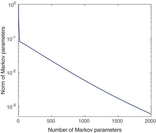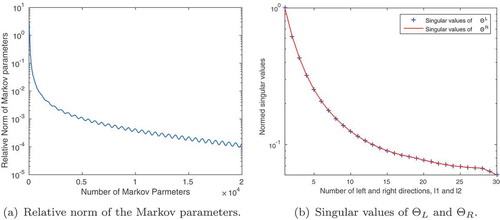We collect $2s=1,000$ Markov parameters. In Figure 1(a), the decay of the normalized Markov parameters is plotted, $\parallel h_i{\parallel }_F/\parallel h_1{\parallel }_F$. 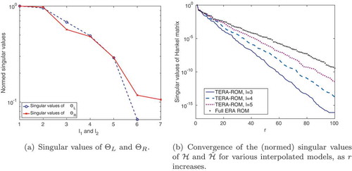We observe a steep initial decay, followed by a slower decay. Figure 1(b) shows the singular values of ${\mathrm{\Theta }}_L$ and ${\mathrm{\Theta }}_R$, which in turn help decide how many input/output directions ${\mathrm{\ell }}_1,{\mathrm{\ell }}_2$ are needed in the TERA framework.

Figure 1. MSD model: The Markov parameters decay slowly in time (a); the singular values of the matrices ${\mathrm{\Theta }}_L$ and ${\mathrm{\Theta }}_R$ help guide the decision about the number of input/output interpolation directions needed (b).

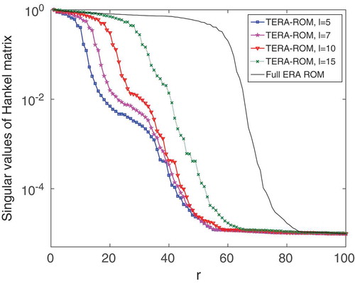
Application of the standard ERA requires computing an SVD of size $15,000\times 15,000$. On the other hand, in TERA, we pick ${\mathrm{\ell }}_1={\mathrm{\ell }}_2=7$, reducing the SVD dimension to $3500\times 3500$. Even though we picked ${\mathrm{\ell }}_1={\mathrm{\ell }}_2=7$ for TERA, we illustrate the leading hundred normalized singular values of both the full Hankel matrix $\mathcal{H}$ and several projected Hankel matrices $\hat{\mathcal{H}}$ in Figure 2 for various ${\mathrm{\ell }}_1$ and ${\mathrm{\ell }}_2$ choices. There is a drastic difference in the decay of the singular values. At the truncation order $r=30$, the singular values of $\hat{\mathcal{H}}$ have already dropped significantly. In contrast, the singular values of the full Hankel matrix start a rapid decay only after $r\approx 60$.

Figure 2. MSD model: The normalized singular values of the Hankel matrices $\mathcal{H}$ and $\hat{\mathcal{H}}$ are shown in decreasing order. With an increasing number of interpolation directions ${\mathrm{\ell }}_1={\mathrm{\ell }}_2$, the singular value decay curves approach the singular value decay of the full Hankel matrix $\mathcal{H}$.

We choose the reduced model order as $r=30$, and apply both ERA and TERA. Theorem 3.4 via the upper bound in (26) can give valuable insight into the success of TERA. Choosing $r=30$, and ${\mathrm{\ell }}_1={\mathrm{\ell }}_2=7$, the actual relative error in the Markov parameters is

$\frac{{\sum }_{i=1}^{2s-1}||h_i-C_r{A}_r^{i-1}{B}_r|{|}_F^2}{{\sum }_{i=1}^{2s-1}||h_i|{|}_F^2}=1.13\times {10}^{-1},$

and the upper bound in (26) yields

$\frac{4\left({\sum }_{i={\mathrm{\ell }}_1+1}^p{\sigma }_i^2({\mathrm{\Theta }}_L)+{\sum }_{i={\mathrm{\ell }}_2+1}^m{\sigma }_i^2({\mathrm{\Theta }}_R)\right)+2\sqrt{r+{\mathrm{\ell }}_1+{\mathrm{\ell }}_2}\cdot {\sigma }_{r+1}(\hat{\mathcal{H}})}{{\sum }_{i=1}^{2s-1}||h_i|{|}_F^2}=8.79\times {10}^{-1}.$

Notably, the error bound is in the same order of magnitude as the actual error. The main contribution to the upper bound results from the truncation of ${\mathrm{\Theta }}_L$ and ${\mathrm{\Theta }}_R$. As a comparison, we also give the actual error and the error bound for the standard $\mathrm{E}\mathrm{R}\mathrm{A}$. While the actual relative error due to the standard ERA is

$\frac{{\sum }_{i=1}^{2s-1}\parallel C_r{A}_r^{i-1}{B}_r-h_i{\parallel }_F^2}{{\sum }_{i=1}^{2s-1}\parallel h_i{\parallel }_F^2}=5.05\times {10}^{-1},$

the upper bound for ERA is

$\frac{{\sigma }_{r+1}(\hat{\mathcal{H}})\cdot \sqrt{r+m+p}}{{\sum }_{i=1}^{2s-1}\parallel h_i{\parallel }_F^2}=1.33\times {10}^0.$

As we shall see again in the next example, Kung’s error bound might not be sharp, and in fact may vary by several orders of magnitude from the true error. Thus, since the error bound is above 100%, it would have been hard to know a priori how well the ROM behaves.

To compare the reduced models due to ERA and TERA, both reduced models are converted back to continuous time, yielding

(29) ${\dot{x}}_r(t)=A_{r,c}{x}_r(t)+B_{r,c}u(t),y_r(t)=C_{r,c}{x}_r(t)+D_{r,c}u(t).$(29)

The full model and the reduced systems (29) obtained from ERA and TERA, respectively, are simulated from zero to $50s$ with zero initial conditions. The input functions were chosen as in [42, Ex. 6.3] to be $u_i(t)=e^{-0.05t}sin(5t)$. Figure 3 shows outputs 6 and 11 of time domain simulations for the full model and both reduced models. Here, the TERA-based reduced model follows the full model outputs accurately. In contrast, the ERA-based reduced-order model responses are far from the actual output and produce erroneous results as shown in Figure 3.

Figure 3. MSD model: Outputs of continuous-time simulations from the full model, and reduced models with $r=30$. In this case, TERA-ROM matches the output of the full order model better, whereas ERA shows strong deviations compared to the full order model.

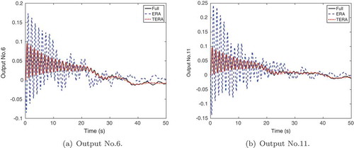
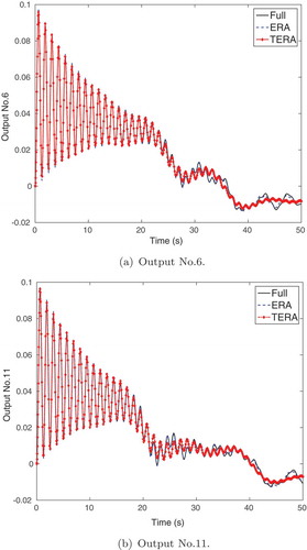
These results illustrate that the reduced order $r=30$ is too low for ERA to produce satisfactory results; thus we increase $r$ to study the performance of ERA more. Based on the plot of the Hankel singular values, Figure 2, the singular values of the full Hankel matrix start decaying at order $r\approx 60$. Figure 4 compares the continuous-time simulations of the full model, and both reduced-order models with $r=60$ (the left and right interpolation directions for TERA are kept at ${\mathrm{\ell }}_1={\mathrm{\ell }}_2=7$). The outputs of the ERA model have now improved in accuracy and mimic the full model outputs accurately.

Figure 4. MSD model: Outputs of continuous-time simulations from the full model, and reduced models with $r=60$. At higher reduced order dimension, ERA performs better, and is visually indistinguishable from the full model.

For a better comparison of the performance across all inputs and outputs, we include Figure 5 below, where we show the Bode plots for the full model, ERA and TERA with ${\mathrm{\ell }}_1={\mathrm{\ell }}_2=10$ and ${\mathrm{\ell }}_1={\mathrm{\ell }}_2=15$. We see that as we increase the interpolation directions, the frequency response of TERA approaches ERA as expected, and the Bode plot is better matched. Note, that the original system has $m=p=30$ inputs and outputs. However, one should observe that even the original full ERA misses the sharp pick of the Bode plot around $\omega =2$ rad/sec. This is unfortunately the best one can do with an ERA setting here. Unlike other data-driven approaches, such as the Loewner framework [28] or data-driven optimal ${\mathcal{H}}_2$ interpolation method TF-IRKA [31], we cannot simply sample the transfer function at various frequencies to have a better/optimal reduced model (and capture the sharp behaviour around $\omega =2$). State-space matrices are assumed not available to start with. All that is available are Markov parameters (data), and the goal is to get a reduced model from this data, which are stable, and have a bound for the sum of squares in the Frobenius norm of the error in the Markov parameters.

Figure 5. MSD model: Transfer function for ERA and TERA where ROMS have order $r=80$, and the TERA models were obtained by interpolating the data with a different number of directions. In plot (a), the original transfer function shows a peak around $\omega =2$. In both (a) and (b), ERA remains unchanged, and we show that TERA approaches the transfer function obtained from ERA as we increase the number of tangential directions.

We have tried several lower order models and observed that we needed to increase the reduced order to around $r=60$ to have a satisfactory reduced model from ERA. This was also reflected in the decay of the singular values in Figure 2. Thus, for this example, TERA produced a better reduced-order model than ERA even with a smaller $r$ value at the same time reducing the effort for the SVD from a $15,000\times 15,000$ matrix to a $3,500\times 3,500$ matrix. For $r=60$, ERA provides a slightly better match in terms of the output of time-domain simulations, yet it still remains more expensive to compute and the advantage of the computational effort for TERA is still persistent. Moreover, the reader should note that a careful balancing of the number of interpolation directions ${\mathrm{\ell }}_1,{\mathrm{\ell }}_2$, and the reduced-order model size $r$, led to a satisfactory accuracy in the ROM, while saving computational time. We shall add though, that in general we do not expect TERA to outperform ERA in accuracy, as it did in this particular case. Nonetheless, since ERA is only optimal in reconstruction, the fact that an improvement in accuracy occurred here, is not contradictory.

4.2. Cooling of steel profiles – Rail model

The model is taken from the Oberwolfach benchmark collection for model reduction [43] and is further described in [44]. The process is modelled by a two-dimensional heat equation with boundary control input. A finite element discretization results in a model $(E,A,B,C)$ with $n=1,357$ states, $m=7$ outputs and $p=6$ outputs. The generalized eigenvalue of $Av=\lambda Ev,v\ne 0$, with largest real part is ${\lambda }_{max}=-1.76\times {10}^{-5}$, which implies that the Markov parameters will decay slowly. It is therefore necessary to sample many Markov parameters to capture enough of the system dynamics. The model is converted to a discrete-time model through the bilinear transformation and simulated to construct $2s=2,000$ Markov parameters. Once again, the original matrices are only used for Markov parameter generation and never enter into the algorithm. Figure 6, shows the normalized decay of the Markov parameters over time, that is, $\parallel h_i{\parallel }_F/\parallel h_1{\parallel }_F$ for $i=1:20:2,000$. The plot can guide the choice of when to stop collecting data. Next, we investigate the performance of ERA/TERA, with reduced-model order $r=20$, unless indicated otherwise. Thus, the standard ERA is applied to the sequence of $2s=2,000$ Markov parameters in ${\mathbb{R}}^{6\times 7}$ requiring an SVD of size $6,000\times 7,000$. Unless otherwise stated, the Markov parameters are projected with ${\mathrm{\ell }}_1={\mathrm{\ell }}_2=4$ tangential directions, so that ${\hat{h}}_i\in {\mathbb{R}}^{4\times 4}$. Therefore, only a singular value decomposition of size $4,000\times 4,000$ has to be computed.

Figure 6. Rail model: Norm (relative) decay of the Markov parameters over time, $||h_i|{|}_F/||h_1|{|}_F$.

Figure 7(a) shows the normalized singular values of the matrices ${\mathrm{\Theta }}_L$ and ${\mathrm{\Theta }}_R$, respectively. In addition to computational cost limitations, the decay of the singular values gives valuable insight for choosing the tangential truncation orders ${\mathrm{\ell }}_1$ and ${\mathrm{\ell }}_2$, since they occur in the error bound in (26). Moreover, in Figure 7(b), we see the convergence of the singular values of Hankel matrix from tangentially interpolated data for various values of ${\mathrm{\ell }}_1$ and ${\mathrm{\ell }}_2$, as the dimension of the reduced-order model $r$ increases. As the size of the Hankel matrix grows the singular values converge to the full model. The first neglected singular value ${\sigma }_{r+1}(\hat{\mathcal{H}})$ enters into the upper bound of the TERA error in Equation (26).

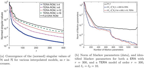
Figure 7. Rail model: The singular values of the matrices ${\mathrm{\Theta }}_L,{\mathrm{\Theta }}_R$ as well as of the Hankel matrix provide insight into truncation of input/output directions, as well as the ROM dimension $r$. In plot (b), for increasing numbers of tangential directions, the singular value decay approaches the behaviour of the ERA model, as expected.

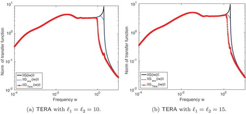
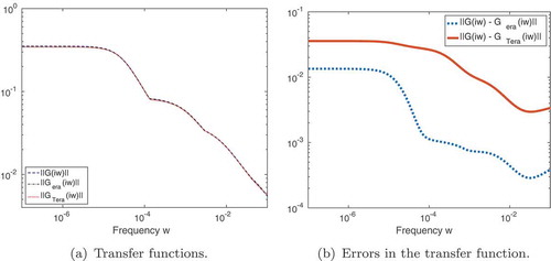
Figure 8 compares the full transfer function $G(i\omega )$ with the reduced-order transfer functions $G_r(i\omega )$ of the ERA and TERA ROMs by showing the amplitude Bode plots. The ${\mathcal{H}}_{\mathrm{\infty }}$ error (where the Hardy-norm $\left|\left|G\right|{|}_{{\mathcal{H}}_{\mathrm{\infty }}}={sup}_{\omega \in \mathbb{R}}\right|\left|G(i\omega )\right|{|}_2$) for TERA is $3.58\times {10}^{-2}$ and similarly $1.36\times {10}^{-2}$ for ERA, which is in the same order of magnitude.

Figure 8. Rail model: Bode plots (transfer function) for full model, and the reduced-order models through ERA and TERA. As seen from (a), the transfer functions in the original scaling are visually identical. Thus, plot (b) shows the error of TERA and ERA with respect to the original transfer function.

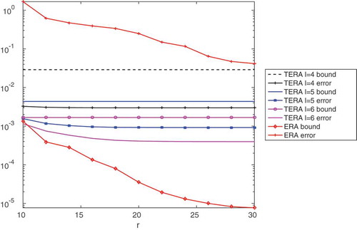
In the following, we shed some light on the behaviour of the error bound for ERA in (12) as well as the TERA error bound in (26). While the true relative error due to TERA with ${\mathrm{\ell }}_1={\mathrm{\ell }}_2=4$ is

$\frac{{\sum }_{i=1}^{2s-1}||h_i-C_r{A}_r^{i-1}{\hat{B}}_r|{|}_F^2}{{\sum }_{i=1}^{2s-1}||h_i|{|}_F^2}=2.98\times {10}^{-3},$

the upper bound from Theorem 3.4 yields

$\frac{4\left({\sum }_{i={\mathrm{\ell }}_1+1}^p{\sigma }_i^2({\mathrm{\Theta }}_L)+{\sum }_{i={\mathrm{\ell }}_2+1}^m{\sigma }_i^2({\mathrm{\Theta }}_R)\right)+2\sqrt{r+{\mathrm{\ell }}_1+{\mathrm{\ell }}_2}\cdot {\sigma }_{r+1}(\hat{\mathcal{H}})}{{\sum }_{i=1}^{2s-1}||h_i|{|}_F^2}=8.54\times {10}^{-2}.$

Even though the upper bound is not too pessimistic, it is not as tight as the previous example. This was expected from the slower decay of the Hankel singular values and the singular values of ${\mathrm{\Theta }}_L$ and ${\mathrm{\Theta }}_R$. On the contrary, the error bound for the standard ERA is rather pessimistic. While the true relative error due to the standard ERA is

$\frac{{\sum }_{i=1}^{2s-1}\parallel C_r{A}_r^{i-1}{B}_r-h_i{\parallel }_F^2}{{\sum }_{i=1}^{2s-1}\parallel h_i{\parallel }_F^2}=3.53\times {10}^{-5},$

the upper bound for ERA is

$\frac{{\sigma }_{r+1}(\hat{\mathcal{H}})\cdot \sqrt{r+m+p}}{{\sum }_{i=1}^{2s-1}\parallel h_i{\parallel }_F^2}=2.50\times {10}^{-1},$

four orders of magnitude higher than the actual error. A more thorough look at the error bound of TERA for various reduced-order model sizes $r$ and interpolation directions ${\mathrm{\ell }}_1$ and ${\mathrm{\ell }}_2$ is given in Figure 9. ERA obviously produces the lowest errors, yet the error bound is almost three orders of magnitudes higher than the true error. For TERA, we see that the error bound and actual error are within the same order of magnitude, yet the method produces higher errors. The error bound in Equation (26) is dominated by the truncated singular values of the matrices ${\mathrm{\Theta }}_L$ and ${\mathrm{\Theta }}_R$, so that there is no significant decay trend of the error bound with increasing order $r$.

Figure 9. Rail model: The error bound of ERA (normalized) from (12) and TERA from (26) versus the actual errors.

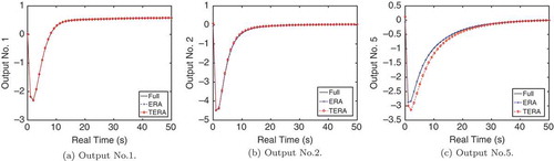
The continuous-time reduced-order models (29) are simulated with an input vector $u(t)\in {\mathbb{R}}^m$ with $u_i(t)=0.2e^{-.005t}$, for $i=1,\dots ,m=7$. For time stepping, we used ode45 in MATLAB with standard error tolerances. The outputs are compared to the outputs of simulations of the full model. Figure 10 shows outputs No. 1, No. 2 and No. 5 computed from the full model as well as the reduced models obtained through both standard ERA and TERA. In addition to reducing the computational time and memory requirements of standard ERA, the TERA framework performs well in time domain simulations. Outputs No. 1 and No. 2 are captured very accurately. While one can observe a deviation in the approximation of output No. 5, the overall behaviour is still approximated well.

Figure 10. Rail model: The plot shows outputs of time domain simulations of the full and reduced-order models. In plot (a) and (b), all three models provide visually identical results, in plot (c), TERA shows a slight deviation for the first 20 s of simulation.

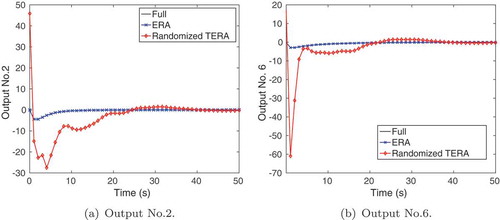
For both models, to show that the success of the selection of projection/tangential directions for TERA via SVD is not random, we generated tangential directions from a random normal distribution (as opposed to using the singular vectors of ${\mathrm{\Theta }}_R$ and ${\mathrm{\Theta }}_L$). This approach gave unsatisfactory results in all the test runs and we, therefore, safely exclude it as a choice for tangential directions. For illustration purposes, for the Rail model, we plotted the results of the continuous-time simulations for output two and six in Figure 11, where random interpolation directions were used for $\hat{\mathcal{H}}$, leading to a rather poor model reduction performance.

Figure 11. Rail model: Time domain simulations of the full and reduced-order models, where the TERA model was obtained by interpolation with random directions. The full model and the ERA model are visually indistinguishable on this scale.

4.3. Indoor-air model for thermal fluid dynamics

We offer a brief explanation for the limitations of the proposed TERA approach by revisiting the indoor-air behaviour model [5] from Example 2.4. The motivation is that it is often not possible to extract system matrices from commercial software, yet one can use SI methods to obtain reduced-order models for the dynamics. Given the size of the problem (input–output dimension as well as data), it would be computationally beneficial to use ERA with tangentially interpolated data. The tools developed earlier can help us decide whether TERA could be applied here.

We consider a similar model as illustrated in Example 2.4. For this problem, $1437$ Markov parameters were obtained by simulating the underlying dynamical system using the ANSYS FLUENT software with a spatial discretization of approximately $200,000$ finite volume elements used in a three dimensional domain. The version of the model we consider here already has a reduced number of outputs, $p=19$, yet similar inputs, $m=26$. Consequently, this would mean that the standard ERA for this model is computationally demanding, requiring an SVD for a matrix of dimension $18,668\times 13,642$; thus reflecting a limitation for the standard ERA itself. Since the internal representation is not available, we cannot provide the same level of detailed comparison as above.

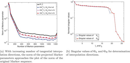
First, we show in Figure 12(a), the norm of the Markov parameters of the full model $||h_i|{|}_F^2$ versus the norm of the interpolated Markov parameters $||{\hat{h}}_i|{|}_F^2$. This shows the information that is retained after the tangential interpolation procedure, which then enters the TERA algorithm. Figure 12(b) shows the decay of the singular values of ${\mathrm{\Theta }}_L$ and ${\mathrm{\Theta }}_R$ to determine the number of necessary interpolation directions. The reader should compare this to Figures 1(b) and 7(a), where a faster decay in the singular values is observed. Since the error bound in Theorem 3.4 contains the summed tail of the neglected singular values of ${\mathrm{\Theta }}_R$ and ${\mathrm{\Theta }}_L$, the upper bound is expected to be loose.

Figure 12. Indoor-air model: A high number of interpolation directions is needed to retain enough information from the sequence of Markov parameters. Especially plot (b) shows that decay of the singular values for ${\mathrm{\Theta }}_L,{\mathrm{\Theta }}_R$ with respect to ${\mathrm{\ell }}_1,{\mathrm{\ell }}_2$ is very slow.

The other ingredient to the error bound in Theorem 3.4 is the first neglected singular value of the full Hankel matrix, ${\sigma }_{r+1}(\hat{\mathcal{H}})$. The singular values of the Hankel matrix from interpolated data are shown in Figure 13(a). As in the previous examples, the Hankel singular values converge to the true values as we increase the interpolation directions ${\mathrm{\ell }}_1={\mathrm{\ell }}_2=\mathrm{\ell }$. However, the convergence is noticeably slower than in the previous two examples. Taken together, one might expect TERA not to yield satisfactory results for small values of $\mathrm{\ell }$; which could hint at the fact that all inputs and outputs are highly relevant for this particular model as we shall see below. In contrast, for large $\mathrm{\ell }$, the computational benefit of using TERA is negligible, in which case one would say that the methods ‘fails’.

Figure 13. Indoor-air model: The TERA models slowly approach the ERA model as the number of interpolation directions ${\mathrm{\ell }}_1={\mathrm{\ell }}_2$ is increased, see plot (a). Part (b) shows that even the identified Markov parameters from a full ERA model do not match the original sequence well.

Following this a priori analysis, in Figure 13(b), we compare the original and identified Markov parameters, using ERA (an expensive computation of the $18,668\times 13,642$ SVD) and TERA with ${\mathrm{\ell }}_1={\mathrm{\ell }}_2=10$. In both cases, $r=300$ is chosen as the ROM model order. We note here that the relative error ${\sum }_k||h_i-C_r{A}_r^k{B}_r|{|}_F^2/{\sum }_k||h_k|{|}_F^2$ is $2.39\times {10}^{-1}$ for ERA and $2.70\times {10}^{-1}$ for TERA. Thus, ERA still performs better, but the errors are still too large for a reduced-order model with good predictive capabilities. In this example, due to several illustrated factors, TERA could not provide a computational benefit to ERA. This illustrates how to approach the problem of deciding whether tangential interpolation of the data prior to SI is beneficial.

5. Conclusions

We modified the standard ERA to handle MIMO systems more efficiently. After the input and output dimensions are reduced by tangential interpolation of the impulse response data, the standard ERA is used on the low dimensional input and output spaces. The observation and control matrices are subsequently lifted back to the original input and output dimensions. The resulting reduced-order model has the original input and output dimensions, and is guaranteed to retain stability. The computational savings for the necessary singular value decomposition are significant, in particular since the complexity of the SVD grows cubically with the size of the Hankel matrix. Moreover, we give criteria to guide the user whether in a particular model using TERA can be beneficial. The a priori error bound in Theorem 3.4 provides a clear picture regarding the contribution of the tangential interpolation error, and the truncation error of the Hankel matrix to the overall error. The numerical findings demonstrate the success of TERA. The algorithm can run with inputs from experiments or black-box code and accurately identify reduced order dynamics.

There are several interesting directions one can pursue. As showed in [6], ERA can be considered a data-driven approximation to balanced truncation. Establishing and understanding a similar connection for TERA might yield other ways of choosing the left and right directions to project the impulse response data. This connection can also help handling the cases where, for example, only the output dimension is massive but there is only a single input. In the setting of balanced truncation, the authors in [45] offered an effective methodology for those situations by employing a numerical quadrature in the computation of one of the gramians involving the other gramian. It will be beneficial to understand the implications for ERA and TERA as well. Moreover, understanding the effect of noise on the TERA computations will also be important.

Disclosure statement

No potential conflict of interest was reported by the authors.

Additional information

Funding

Research supported in part by the Energy Efficient Buildings Hub under DOE contract DE-EE0004261.

Notes

1. MATLAB and Statistics Toolbox Release 2015b, The MathWorks, Inc., Natick, Massachusetts, United States.

2. We follow the original ERA notation and assume a standard state-space, that is, the E-term is E = I. This makes the notation involving Markov parameters and the Hankel matrix much simpler. The theory can be extended to the general case. One of the numerical examples in Section 4 has E ≠ I.

3. We use this term to refer to the singular values of the Hankel matrix.

References

- I. Houtzager, J. Van Wingerden, and M. Verhaegen, Recursive predictor-based subspace identification with application to the real-time closed-loop tracking of flutter, IEEE Trans. Control Syst. Technol. 20 (2012), pp. 934–949. doi:10.1109/TCST.2011.2157694
- D.C. Rebolho, E.M. Belo, and F.D. Marques, Aeroelastic parameter identification in wind tunnel testing via the extended eigensystem realization algorithm, J. Vib. Control 20 (2014), pp. 1607–1621. doi:10.1177/1077546312474015
- M. Döhler and L. Mevel, Fast multi-order computation of system matrices in subspace-based system identification, Control Eng. Pract. 20 (2012), pp. 882–894. doi:10.1016/j.conengprac.2012.05.005
- J.M. Caicedo, S. Dyke, and E. Johnson, Natural excitation technique and eigensystem realization algorithm for phase I of the IASC-ASCE benchmark problem: Simulated data, J. Eng. Mech. 130 (2004), pp. 49–60. doi:10.1061/(ASCE)0733-9399(2004)130:1(49)
- J. Borggaard, E. Cliff, and S. Gugercin, Model reduction for indoor-air behavior in control design for energy-efficient buildings, Proceedings of the American Control Conference, Montreal, 2012, pp. 2283–2288. ISBN 9781457710957
- Z. Ma, S. Ahuja, and C. Rowley, Reduced-order models for control of fluids using the eigensystem realization algorithm, Theor. Comput. Fluid Dyn. 25 (2011), pp. 233–247. doi:10.1007/s00162-010-0184-8
- F. Juillet, P. Schmid, and P. Huerre, Control of amplifier flows using subspace identification techniques, J. Fluid. Mech. 725 (2013), pp. 522–565. doi:10.1017/jfm.2013.194
- C. Wales, A. Gaitonde, and D. Jones, Stabilisation of reduced order models via restarting, Int. J. Numer. Methods Fluids 73 (2013), pp. 578–599. doi:10.1002/fld.v73.6
- J. Mendel, Minimum-variance deconvolution, IEEE Trans. Geosci. Remote Sensing GE-19 (1981), pp. 161–171. doi:10.1109/TGRS.1981.350346
- M. Viberg, Subspace-based methods for the identification of linear time-invariant systems, Automatica 31 (1995), pp. 1835–1851. doi:10.1016/0005-1098(95)00107-5
- S. Qin, An overview of subspace identification, Comput. Chem. Eng. 30 (2006), pp. 1502–1513. doi:10.1016/j.compchemeng.2006.05.045
- E. Reynders, System identification methods for (operational) modal analysis: Review and comparison, Arch. Comput. Methods Eng. 19 (2012), pp. 51–124. doi:10.1007/s11831-012-9069-x
- S.Y. Kung, A new identification and model reduction algorithm via singular value decomposition, Proceedings of 12th Asilomar Conference on Circuits, Systems & Computers, Pacific Grove, CA, 1978, pp. 705–714. IEEE.
- J.-N. Juang and R. Pappa, An eigensystem realization algorithm for modal parameter identification and model reduction, J. Guidance, Control, Dyn. 8 (1985), pp. 620–627. doi:10.2514/3.20031
- G. Pitstick, J. Cruz, and R. Mulholland, Approximate realization algorithms for truncated impulse response data, IEEE Trans. Acoust. Speech Signal Process. 34 (1986), pp. 1583–1588. doi:10.1109/TASSP.1986.1164997
- R. Longman and J.-N. Juang, Recursive form of the eigensystem realization algorithm for system identification, J. Guidance, Control, Dyn. 12 (1989), pp. 647–652. doi:10.2514/3.20458
- J. Singler, Model reduction of linear PDE systems: A continuous time eigensystem realization algorithm, Proceedings of the American Control Conference, Montreal, 2012, pp. 1424–1429.
- K. Willcox and J. Peraire, Balanced model reduction via the proper orthogonal decomposition, AIAA J. 40 (2002), pp. 2323–2330. doi:10.2514/2.1570
- C. Rowley, Model reduction for fluids, using balanced proper orthogonal decomposition, Int. J. Bifur. Chaos 15 (2005), pp. 997–1013. doi:10.1142/S0218127405012429
- D. Yu and S. Chakravorty, A randomized proper orthogonal decomposition technique, arXiv preprint arXiv:1312.3976, 2013.
- A.C. Antoulas, Approximation of Large-Scale Dynamical Systems, Advances in Design and Control Society for Industrial and Applied Mathematics, Philadelphia, PA, 2005.
- U. Baur, P. Benner, and L. Feng, Model order reduction for linear and nonlinear systems: A system-theoretic perspective, Arch. Comput. Methods Eng. 21 (2014), pp. 331–358. doi:10.1007/s11831-014-9111-2
- A.C. Antoulas, C.A. Beattie, and S. Gugercin, Interpolatory model reduction of large-scale dynamical systems, in Efficient Modeling and Control of Large-Scale Systems, J. Mohammadpour and M.K. Grigoriadis, eds., Springer US, Boston, MA, 2010, pp. 3–58.
- B. Moore, Principal component analysis in linear systems: Controllability, observability, and model reduction, IEEE Trans. Automat. Contr. 26 (1981), pp. 17–32. doi:10.1109/TAC.1981.1102568
- C. Mullis and R. Roberts, Synthesis of minimum roundoff noise fixed point digital filters, IEEE Trans. Circuits Syst. 23 (1976), pp. 551–562. doi:10.1109/TCS.1976.1084254
- S. Gugercin, A. Antoulas, and C.A. Beattie, model reduction for large-scale linear dynamical systems, SIAM J. Matrix Anal. Appl. 30 (2008), pp. 609–638. doi:10.1137/060666123
- K. Glover, All optimal Hankel-norm approximations of linear multivariable systems and their L,∞-error bounds, Int. J. Control 39 (1984), pp. 1115–1193. doi:10.1080/00207178408933239
- A. Mayo and A. Antoulas, A framework for the solution of the generalized realization problem, Linear Algebra Appl. 425 (2007), pp. 634–662. doi:10.1016/j.laa.2007.03.008
- B. Gustavsen and A. Semlyen, Rational approximation of frequency domain responses by vector fitting, IEEE Trans. Power Deliv. 14 (1999), pp. 1052–1061. doi:10.1109/61.772353
- Z. Drmač, S. Gugercin, and C. Beattie, Quadrature-based vector fitting for discretized approximation, SIAM J. Sci. Comput. 37 (2015), pp. A625–A652. doi:10.1137/140961511
- C. Beattie and S. Gugercin, Realization–independent approximation, Proceedings of the 51st IEEE Conference on Decision & Control, Maui, HI, IEEE, 2012, pp. 4953–4958.
- C. Sanathanan and J. Koerner, Transfer function synthesis as a ratio of two complex polynomials, IEEE Trans. Autom. Control 8 (1963), pp. 56–58. doi:10.1109/TAC.1963.1105517
- M. Berljafa and S. Güttel, Generalized rational Krylov decompositions with an application to rational approximation, SIAM J. Matrix Anal. Appl. 36 (2015), pp. 894–916. doi:10.1137/140998081
- Z. Drmač, S. Gugercin, and C. Beattie, Vector fitting for matrix-valued rational approximation, SIAM J. Scientific Comput. 37 (2015), pp. A2346–A2379. doi:10.1137/15M1010774
- L.M. Silverman, Realization of linear dynamical systems, IEEE Trans. Automat. Contr. 16 (1971), pp. 554–567. doi:10.1109/TAC.1971.1099821
- G. Golub and C.F. Van Loan, Matrix Computations, Johns Hopkins University, Press, Baltimore, MD, 1996, pp. 374–426.
- C.A. Beattie and S. Gugercin, Model reduction by rational interpolation, in Model Reduction and Approximation for Complex Systems, P. Benner, A. Cohen, M. Ohlberger, and K. Willcox, eds., Marseille, 2014. Available at http://arxiv.org/abs/1409.2140.
- P. Feldmann and F. Liu, Sparse and efficient reduced order modeling of linear subcircuits with large number of terminals, in IEEE/ACM International Conference on Computer Aided Design, 2004. ICCAD-2004, 2004, pp. 88–92.
- P. Liu, S.X. Tan, B. Yan, and B. McGaughy, An extended SVD-based terminal and model order reduction algorithm, Proceedings of the 2006 IEEE International Behavioral Modeling and Simulation Workshop San Jose, CA, 2006, pp. 44–49.
- P. Benner and A. Schneider, Model reduction for linear descriptor systems with many ports, in Progress in Industrial Mathematics at ECMI 2010, M. Günther, A. Bartel, M. Brunk, S. Schöps, M. Striebel, eds., Springer, Berlin, 2012, pp. 137–143.
- U. Al-Saggaf and G. Franklin, Model reduction via balanced realizations: An extension and frequency weighting techniques, IEEE Trans. Automat. Contr. 33 (1988), pp. 687–692. doi:10.1109/9.1280
- S. Gugercin, R. Polyuga, C. Beattie, and A. Van Der Schaft, Structure-preserving tangential interpolation for model reduction of port-Hamiltonian systems, Automatica 48 (2012), pp. 1963–1974. doi:10.1016/j.automatica.2012.05.052
- IMTEK - Simulation, Oberwolfach benchmark collection, 2003. Available at http://www.simulation.uni-freiburg.de/downloads/benchmark.
- A. Unger and F. Tröltzsch, Fast solution of optimal control problems in the selective cooling of steel, ZAMM Z. Angew. Math. Mech. 81 (2001), pp. 447–456. doi:10.1002/(ISSN)1521-4001
- P. Benner and A. Schneider, Balanced truncation for descriptor systems with many terminals, Max Planck Institute Magdeburg Preprint MPIMD/13-17, 2013. Available at http://www2.mpi-magdeburg.mpg.de/preprints/2013/MPIMD13-17.pdf.