Structure preserving model order reduction of large sparse second-order index-1 systems and application to a mechatronics model

ABSTRACT

Nowadays, mechanical engineers heavily depend on mathematical models for simulation, optimization and controller design. In either of these tasks, reduced dimensional formulations are obligatory in order to achieve fast and accurate results. Usually, the structural mechanical systems of machine tools are described by systems of second-order differential equations. However, they become descriptor systems when extra constraints are imposed on the systems. This article discusses efficient techniques of Gramian-based model-order reduction for second-order index-1 descriptor systems. Unlike, our previous work, here we mainly focus on a second-order to second-order reduction technique for such systems, where the stability of the system is guaranteed to be preserved in contrast to the previous approaches. We show that a special choice of the first-order reformulation of the system allows us to solve only one Lyapuov equation instead of two. We also discuss improvements of the technique to solve the Lyapunov equation using low-rank alternating direction implicit methods, which further reduces the computational cost as well as memory requirement. The proposed technique is applied to a structural finite element method model of a micro-mechanical piezo-actuators-based adaptive spindle support. Numerical results illustrate the increased efficiency of the adapted method.

KEYWORDS:

• Model-order reduction
• mechatronic system
• balanced truncation
• Lyapunov equations
• large-scale
• differential algebraic system

1. Introduction

This article discusses an efficient technique for model-order reduction (MOR) of large-scale sparse second-order index-1 descriptor systems. Mainly, we focus on second-order to second-order balancing of such systems, in order to preserve the structure of the original model. We consider second-order systems of the form

(1) $\begin{array}{c}\underset{ℳ}{\underbrace{\left[\begin{array}{cc}{M}_1& 0\\ 0& 0\end{array}\right]}}\left[\begin{array}{c}\ddot{z}(t)\\ \ddot{\phi }(t)\end{array}\right]+\underset{\mathcal{D}}{\underbrace{\left[\begin{array}{cc}{D}_1& 0\\ 0& 0\end{array}\right]}}\left[\begin{array}{c}\dot{z}(t)\\ \dot{\phi }(t)\end{array}\right]+\underset{\mathcal{K}}{\underbrace{\left[\begin{array}{cc}{K}_{11}& K_{12}\\ K_{12}^T& K_{22}\end{array}\right]}}\left[\begin{array}{c}z(t)\\ \phi (t)\end{array}\right]=\underset{\mathscr{H}}{\underbrace{\left[\begin{array}{c}{B}_1\\ B_2\end{array}\right]}}u(t),\\ y(t)=\underset{{\mathscr{H}}^T}{\underbrace{\left[\begin{array}{cc}{B}_1^T& B_2^T\end{array}\right]}}\left[\begin{array}{c}z(t)\\ \phi (t)\end{array}\right]+D_{a}u(t)\mathrm{,}\end{array}$(1)

where $z(t)\in {\mathbb{R}}^{n_1}$, $\phi (t)\in {\mathbb{R}}^{n_2}$ are the states, $\mathcal{M},\mathcal{D}\mathrm{a}\mathrm{n}\mathrm{d}\mathcal{K}\in {\mathbb{R}}^{n\times n}$ are the finite element method (FEM)-matrices, $\mathcal{H}\in {\mathbb{R}}^{n\times p}$ is the input matrix and the output matrix is ${\mathcal{H}}^T$, i.e. we assume collocated actuators and sensors. The corresponding control inputs and measurement outputs to the system are denoted by u(t) and y(t), respectively. The matrix $D_a\in {\mathbb{R}}^{m\times p}$ represents the direct feedthrough from the input to the output. The matrices $\mathcal{M},\mathcal{D},\mathcal{K}$ and $\mathcal{H}$ are sparse and the first three are symmetric. Moreover, we assume the matrix block K₂₂ to be nonsingular. We call (1) an index-1 system due to the analogy to first-order index-1 (see the next section) linear time-invariant (LTI) systems. See, e.g. [2, Chapter 2] and the references therein about the index of such structured descriptor systems. The dynamical system (1) arises, e.g. in mechatronics, where mechanical and electrical components are coupled with each other. In the specific case of the model example we use in the numerical experiments, the index-1 character results from the multiphysics application with very different timescales. This allows to treat one variable by a (quasi-)stationary analysis, while the other is covered fully dynamic.

If the model is very large, performing the simulation with it requires prohibitively high computational effort or is simply impossible due to the limited computer memory. Therefore, reducing the size of the system is unavoidable for fast simulation. A classical approach to find a reduced-order model (ROM) of second-order index-1 descriptor systems is to first rewrite (1) in first-order form. Then MOR techniques are applied to find a reduced first-order state space system [1]. Under these circumstances, since the block structure of the original model is obfuscated in the reduced model, one cannot go back to the second-order representation if it is desired, to use software designed for second-order systems as, e.g. in flexible multibody simulations.

During the recent years, structure preserving MOR of second-order systems received a lot of attention, see e.g. [3–6] and the references therein. But, all of those approaches are only for standard second-order systems. As in our earlier work [1,7] on this model, also in this article, our goal is to apply MOR to the high dimensional model in (1) and replace it by the substantially lower dimensional model

(2) $\begin{array}{l}\widehat{M}\ddot{\widehat{z}}(t)+\widehat{D}\dot{\widehat{z}}(t)+\widehat{K}\widehat{z}(t)=\widehat{H}u(t),\\ \widehat{y}(t)={\widehat{H}}^T\widehat{z}(t)+{\widehat{D}}_{a}u(t),\end{array}$(2)

where $\hat{M},\hat{D},\hat{K}\in {\mathbb{R}}^{l\times l}$, $\hat{H}\in {\mathbb{R}}^{l\times p}$ and $l\ll n$. It is required that $∥y-\hat{y}∥$ is small and the ROM preserves necessary properties, e.g. stability, passivity and symmetry of the original model.

This article is concerned with balancing-based structure-preserving MOR of the second-order index-1 system (1). The central idea of this method is to truncate the less important states from the system, which correspond to the negligible system Hankel singular values (HSVs). The system HSVs are the square roots of the eigenvalues of the product of the controllability and observability Gramians [8] or equivalently the singular values of the product of the two Gramian factors [9]. A system is balanced if both the Gramians are identical and diagonal with decreasingly ordered entries which are the system’s HSVs. The magnitudes of the HSVs have direct relations to the energy contributions of the corresponding state components in the total input–output behaviour of the system. The smaller the value, the lower the energy portion is and thus the less important the state component.

It is known that the most expensive part in this particular MOR method is to solve the two Lyapunov equations determining the system Gramian factors, which are the key ingredients in the derivation of the truncating matrices for forming the ROM. For a large sparse LTI system, the LRCF-ADI (low-rank Cholesky factor-alternating direction implicit) method [10,11] is one efficient method to compute these Gramian factors. We have already investigated this in [7] for a large sparse second-order index-1 descriptor system. In contrast to [7], in this article, the LRCF-ADI method is updated by exploiting the symmetry properties of the systems, and computing real Gramian factors applying the ideas from [12]. Moreover, we use the residual factor-based stopping criterion [13] to terminate the LRCF-ADI iteration. The presented algorithm to compute the low-rank Gramian factor is based on the second-order index-1 descriptor system (1).

The proposed techniques are applied to a piezo-actuated structural FEM model of a certain building block of a parallel kinematic machine tool. Numerical results illustrate the superiority of the new technique compared to our results in [7].

2. Model example

We investigate a part of the experimental machine tool as shown in Figure 1. It is a complex system, where a piezo-actuator-based adaptive spindle support (ASS) is mounted on a parallel kinematic machine in order to gain additional positioning freedom and accuracy during machining operations (see [14,15] for more details). The important purpose of the piezo-sensor and -actuator is to control active vibration or shunt damping so that the machine can ensure a high-quality product. For analysing the mechanical design and performance of the ASS, a mathematical model as in (1) is formed using the FEM, where $\mathcal{M}$, $\mathcal{D}$ and $\mathcal{K}$ are the mass, damping and stiffness matrices, respectively. The time-dependent state vector z(t) consists of the components of mechanical displacements and $\phi (t)$ are the electrical charges. Separating the mechanical and electrical parts, M₁, D₁ and K₁₁ are, respectively, mechanical mass, mechanical damping and mechanical stiffness matrices. The matrix K is composed of mechanical (K₁₁), electrical (K₂₂) and coupling (K₁₂) terms. The general force quantities (mechanical forces and electrical charges) are chosen as the input quantities $u$, and the corresponding general displacements (mechanical displacements and electrical potential) are the output quantities $y$. The total mass matrix contains zeros at the locations of the electric potential equations. More precisely, the electric potential (degrees of freedom [DoF] for the electrical part) is not associated with an inertia. The equation of motion of the mechanical system in (1) can be found in [16]. This equation results from a finite element discretization of the balance equations. For piezo-mechanical systems, these are the mechanical balance of momentum (with inertia term) and the electro-static balance. From this, the electric potential without inertia term is obtained. Thus, for the whole system (mechanical and electrical DoF) the mass matrix has rank deficiency. There are several ways to transform (1) into its equivalent first-order forms, see e.g. [2] for a selection. In this article, we prefer the following representation:

(3) $\mathcal{E}\dot{\xi }(t)=\mathcal{A}\xi (t)+\mathcal{B}u(t),y(t)={\mathcal{B}}^T\xi (t)+D_{a}u(t),$(3)

Figure 1. (a) The adaptive spindle support (CAD model) and (b) real component mounted on a parallel-kinematic machine [14].

where

(4) $\mathcal{E}=\left[\begin{array}{ccc}0& M_1& 0\\ M_1& D_1& 0\\ 0& 0& 0\end{array}\right],\mathcal{A}=\left[\begin{array}{ccc}{M}_1& 0& 0\\ 0& -K_{11}& -K_{12}\\ 0& -K_{12}^T& -K_{22}\end{array}\right],\mathcal{B}=\left[\begin{array}{c}0\\ B_1\\ B_2\end{array}\right],\mathrm{a}\mathrm{n}\mathrm{d}\xi (t)=\left[\begin{array}{c}\dot{z}(t)\\ z(t)\\ \phi (t)\end{array}\right].$(4)

The advantage of this representation is that if all coefficient matrices in system (1) are symmetric, then so is the matrix in (3). Moreover, the input-output matrices are still transposes of each other after the transformation. This fact can be exploited in the solvers and the MOR process. It accelerates the computations and allows to preserve stability in the reduced-order model, which can not be guaranteed for general second-order systems [3].

3. The BT method for second-order systems and related issues

In this section, we briefly review the BT method for second-order LTI systems

(5) $\begin{array}{rl}& M\ddot{x}(t)+D\dot{x}(t)+Kx(t)=Hu(t),\\ & y(t)=Lx(t)+D_{s}u(t),\end{array}$(5)

where M, D and K are nonsingular, and x(t) is the n dimensional state vector. Transforming (5) into first-order form yields

(6) $\begin{array}{cc}\underset{E}{\underbrace{\left[\begin{array}{cc}0& M\\ M& D\end{array}\right]}}\underset{\dot{\zeta }(t)}{\underbrace{\left[\begin{array}{c}\ddot{x}(t)\\ \dot{x}(t)\end{array}\right]}}& =\underset{A}{\underbrace{\left[\begin{array}{cc}M& 0\\ 0& -K\end{array}\right]}}\underset{\zeta (t)}{\underbrace{\left[\begin{array}{c}\dot{x}(t)\\ x(t)\end{array}\right]}}+\underset{B}{\underbrace{\left[\begin{array}{c}0\\ H\end{array}\right]}}u(t),\\ & y(t)=\underset{C}{\underbrace{\left[\begin{array}{cc}0& L\end{array}\right]}}\left[\begin{array}{c}\dot{x}(t)\\ x(t)\end{array}\right]+D_{s}u(t).\end{array}$(6)

The controllability Gramian $W_c\in R^{2n\times 2n}$ and the observability Gramian $W_o\in R^{2n\times 2n}$ for system (6) are the solutions of the Lyapunov equations

(7) $A{W}_c{E}^T+E{W}_c{A}^T=-B{B}^T\mathrm{a}\mathrm{n}\mathrm{d}{A}^T{W}_{o}E+E^T{W}_{o}A=-C^{T}C.$(7)

The Gramians can also be defined from a physical point of view. Defining an energy function

$J(u)=\underset{-\mathrm{\infty }}{\overset{0}{\int }}{u}^{\ast }(t)u(t)\mathrm{d}t,$

Glover in [8] shows that the optimal value of the minimization problem

(8) $\begin{array}{cc} & \underset{u}{\mathrm{m}\mathrm{i}\mathrm{n}} J(u)\\ & \mathrm{s}.\mathrm{t}.E\dot{\zeta }(t)=A\zeta (t)+\mathrm{B}\mathrm{u}(t),\zeta (0)={\zeta }_0,\end{array}$(8)

is

(9) ${\zeta }_0^T{W}_c^{-1}{\zeta }_0.$(9)

This is the required minimal energy to steer the state of system (6) from $t=-\mathrm{\infty }$ to the state ${\zeta }_0$ at time t = 0. Based on the optimization problem (8), the Gramians for the second-order system (5) are first defined in [17]. Let us consider the following optimization problems

(10) $\begin{array}{cc} & \underset{{\dot{x}}_0}{\mathrm{m}\mathrm{i}\mathrm{n}}\underset{u}{\mathrm{m}\mathrm{i}\mathrm{n}} J(u)\\ & \mathrm{s}.\mathrm{t}.M\ddot{x}(t)+D\dot{x}(t)+Kx(t)=\mathrm{H}\mathrm{u}(t),\dot{x}(0)={\dot{x}}_0,\end{array}$(10)

and

(11) $\begin{array}{cc} & \underset{x_0}{\mathrm{m}\mathrm{i}\mathrm{n}}\underset{u}{\mathrm{m}\mathrm{i}\mathrm{n}} J(u)\\ & \mathrm{s}.\mathrm{t}.M\ddot{x}(t)+D\dot{x}(t)+Kx(t)=\mathrm{H}\mathrm{u}(t),x(0)=x_0.\end{array}$(11)

Due to the structure of system (6), the controllability Gramian can be compatibly partitioned as

$W_c=\left[\begin{array}{cc}{P}_v& P_o\\ P_o^T& P_p\end{array}\right].$

The authors in [17] (see also [18]), prove that the optimal solution to problem (10) is ${\dot{x}}_0{P}_v^{-1}{\dot{x}}_0$, which is the minimal energy required to reach the given velocity ${\dot{x}}_0$ over all past inputs and initial values. The solution of problem (11) is $x_0{P}_p^{-1}{x}_0$, which is the minimal energy required to reach the given position x₀ over all past inputs and initial values. Here, P_v and P_p are defined as second-order controllability velocity Gramian and position Gramian, respectively. Analogously, one can interpret the observability Gramian $W_o$ by using duality arguments. Then partitioning $W_o$ as

$W_o=\left[\begin{array}{cc}{Q}_v& Q_o\\ Q_o^T& Q_p\end{array}\right],$

we obtain the observability velocity Gramian $Q_v$ and position Gramian $Q_p$.

We consider R as a low-rank controllability Gramian factor such that $W_c\approx R{R}^T$. The structure of the first-order system allows us to split $R$ as

(12) $R={\left[\begin{array}{cc}{R}_v^T& R_p^T\end{array}\right]}^T.$(12)

Therefore, the controllability Gramian can be written as

$W_c=\left[\begin{array}{cc}{P}_v& P_o\\ P_o^T& P_p\end{array}\right]\approx R{R}^T=\left[\begin{array}{c}{R}_v\\ R_p\end{array}\right]\left[\begin{array}{cc}{R}_v^T& R_p^T\end{array}\right]=\left[\begin{array}{cc}{R}_v{R}_v^T& R_v{R}_p^T\\ R_p{R}_v^T& R_p{R}_p^T\end{array}\right].$

Hence, we have

$P_v\approx R_v{R}_v^T\mathrm{a}\mathrm{n}\mathrm{d}{P}_p\approx R_p{R}_p^T.$

Similarly, considering $W_o\approx L{L}^T$, we find

$Q_v\approx L_v{L}_v^T\mathrm{a}\mathrm{n}\mathrm{d}{Q}_p\approx L_p{L}_p^T,$

where $L={\left[\begin{array}{cc}{L}_v^T& L_p^T\end{array}\right]}^T$. Apparently, R_v and R_p are obtained from the first n rows and the lower n rows of R, respectively. Analogously, L_v and L_p can be obtained from the first n rows and the lower n rows of the low-rank observability Gramian factor L. Once we have $R_{\alpha }$ and $L_{\beta }$, where $\alpha ,\beta \in \{v,p\}$, the balancing transformation can be formed using the SVD

(13) $R_{\alpha }^{T}M{L}_{\beta }=U_{\alpha \beta }{\mathrm{\Sigma }}_{\alpha \beta }{V}_{\alpha \beta }^T=\left[\begin{array}{cc}{U}_{\alpha \beta ,1}& U_{\alpha \beta ,2}\end{array}\right]\left[\begin{array}{cc}{\mathrm{\Sigma }}_{\alpha \beta ,1}& \\ & {\mathrm{\Sigma }}_{\alpha \beta ,2}\end{array}\right]\left[\begin{array}{c}{V}_{\alpha \beta ,1}^T\\ V_{\alpha \beta ,2}^T\end{array}\right],$(13)

and defining

(14) $T_L:=L_{\beta }{U}_{\alpha \beta ,1}{\mathrm{\Sigma }}_{\alpha \beta ,1}^{-1/2},T_R:=R_{\alpha }{V}_{\alpha \beta ,1}{\mathrm{\Sigma }}_{\alpha \beta ,1}^{-1/2}.$(14)

Here $U_{\alpha \beta ,1}$ and $V_{\alpha \beta ,1}$ are composed of the leading k columns of $U_{\alpha \beta }$ and $V_{\alpha \beta }$, respectively and ${\mathrm{\Sigma }}_{\alpha \beta ,1}$ is the first $k\times k$ block of the matrix ${\mathrm{\Sigma }}_{\alpha \beta }$. Now, the ROM as in (2) can be formed by constructing the matrices of reduced dimensions:

(15) $\begin{array}{c}\hat{M}=T_L^{T}M{T}_R,\hat{D}=T_L^{T}D{T}_R,\hat{K}=T_L^{T}K{T}_R, \hat{H}=T_L^{T}H\mathrm{a}\mathrm{n}\mathrm{d}\hat{L}=L{T}_R.\end{array}$(15)

Algorithm 1:

GLRCF-ADI for solving $FX{\stackrel{⌣}{E}}^T+\stackrel{⌣}{E}X{F}^T=-N{N}^T$.

 Input: $F,\stackrel{⌣}{E},N$, shift parameters ${\left\{{\mu }_i\right\}}_{i=1}^J\subset {\mathbb{C}}_{-}$.

 Output: $Z=Z_i$ such that $X\approx Z{Z}^T$.

1 $W_0=N,Z_0=[],i=1$.

2 while $∥W_{i-1}^T{W}_{i-1}∥\ge \mathrm{t}\mathrm{o}l$ or $i\le i_{\mathrm{m}\mathrm{a}\mathrm{x}}$ do

3 Solve $(F+{\mu }_i\stackrel{⌣}{E})V_i=W_{i-1}$ for $V_i$.

4 if $\mathrm{I}\mathrm{m}({\mu }_i)=0$ then

5 $Z_i=\left[Z_{i-1},\sqrt{-2{\mu }_i}{V}_i\right].$

6 $W_i=W_{i-1}-2Re\left({\mu }_i\right)\stackrel{⌣}{E}{V}_i.$

7 else

8 ${\gamma }_i=2\sqrt{-Re\left({\mu }_i\right)},{\delta }_i=\frac{Re\left({\mu }_i\right)}{Im\left({\mu }_i\right)}$.

9 $Z_{i+1}=[Z_{i-1},{\gamma }_j\left(Re\left(V_i\right)+{\delta }_j\mathrm{I}\mathrm{m}\left(V_i\right)\right),{\gamma }_i\sqrt{\left({\delta }_i^2+1\right)}\cdot \mathrm{I}\mathrm{m}\left(V_i\right)]$.

10 $W_{i+1}=W_{i-1}+{\gamma }_i^2\stackrel{⌣}{E}\left(Re\left(V_i\right)+{\delta }_i\mathrm{I}\mathrm{m}\left(V_i\right)\right)$.

11 i = i + 1

12 i = i + 1

When $\alpha =\beta =v$, the balancing technique by the above procedure is called velocity–velocity (VV) balancing. Likewise, position–position (PP) balancing is obtained, if $\alpha =\beta =p$, velocity–position (VP) balancing is obtained if $\alpha =v,\beta =p$ and position–velocity (PV) balancing is obtained if $\alpha =p,\beta =v$. See, e.g. [3] for more details.

The fundamental drawback of the balancing based model reduction is the necessity to compute the two Gramian factors by solving two Lyapunov equations. Among several approaches, the LRCF-ADI method has been developed that allows to exploit the fact that often all coefficient matrices are sparse and the number of inputs and outputs are very small compared to the number of DoFs. We refer the reader to [10,19] and the references therein for details on the LRCF-ADI approach. Recently, this prominent method has been updated by exploiting the ideas of computing real low-rank Gramian factors [12] and a low-rank residual based stopping criterion. For convenience, the updated version of the LRCF-ADI (GLRCF-ADI) algorithm is summarized in Algorithm 3.

This algorithm either successively computes $Z=R$ for $(\stackrel{⌣}{E},F,N)=(E,A,B)$ or Z = L for $(\stackrel{⌣}{E},F,N)=(E^T,A^T,C^T)$. In this algorithm, ${\left\{{\mu }_i\right\}}_{i=1}^J$ are called the ADI shift parameters or simply shift parameters [11]. A set of good shift parameters is necessary for fast convergence of the algorithm. Although several strategies are available in the literature (see e.g. [20] and the references therein), in this article, we restrict ourselves to the heuristic approach introduced in [11] and an adaptive choice following [20].

4. The BT method for second-order index-1 systems

This section discusses the balancing based model reduction methods for the second-order index-1 descriptor system (1). For a survey on balancing-related MOR methods for general descriptor systems, we refer to the recent survey [21]. In this case first, we transform the second-order index-1 descriptor system (1) into a standard system (5), where

(16) $\begin{array}{cc} & M=M_1,D=D_1,K=K_{11}-K_{12}{K}_{22}^{-1}{K}_{12}^T,\\ & H=B_1-K_{12}{K}_{22}^{-1}{B}_2,L=H^T\mathrm{a}\mathrm{n}\mathrm{d}{D}_s=D_a+C_2{K}_{22}^{-1}{B}_2.\end{array}$(16)

Note that K, H will then usually be dense matrices. Section 5 gives details on how to avoid forming them.

The first-order representation of this standard second-order model is obtained as in (6). Since the first-order form is symmetric (A^T = A, E^T = E) and the input–output matrices are transposes of each other (C = b, C = B^T), the controllability Gramian and the observability Gramian coincide, i.e. W_c = W_o = W and only one Lyapunov equation

(17) $AWE+EWA=-B{B}^T$(17)

needs to be solved. Therefore, we can consider

(18) ${\left[\begin{array}{cc}{R}_v^T& R_p^T\end{array}\right]}^T={\left[\begin{array}{cc}{L}_v^T& L_p^T\end{array}\right]}^T={\left[\begin{array}{cc}{Z}_v^T& Z_p^T\end{array}\right]}^T.$(18)

Note that the following section will discuss how to solve the Lyapunov equation (17) efficiently. Once we have computed Z_v and Z_p by solving the Lyapunov equation, following (13) and (14) we can compute four types of balancing transformations as shown in Table 1.

Table 1. Balancing transformations for the second-order index-1 descriptor systems.

Type	SVD	Left proj. TL	Right proj. TR
VV	$Z_v^T{M}_1{Z}_v=U_{vv}{\mathrm{\Sigma }}_{vv}{U}_{vv}^T$	$Z_v{U}_{vv,1}{\mathrm{\Sigma }}_{vv,1}^{-1/2}$	$Z_v{U}_{vv,1}{\mathrm{\Sigma }}_{vv,1}^{-1/2}$
PP	$Z_p^T{M}_1{Z}_p=U_{pp}{\mathrm{\Sigma }}_{pp}{U}_{pp}^T$	$Z_p{U}_{pp,1}{\mathrm{\Sigma }}_{pp,1}^{-1/2}$	$Z_p{U}_{pp,1}{\mathrm{\Sigma }}_{pp,1}^{-1/2}$
VP	$Z_v^T{M}_1{Z}_p=U_{vp}{\mathrm{\Sigma }}_{vp}{V}_{vp}^T$	$Z_p{U}_{vp,1}{\mathrm{\Sigma }}_{vp,1}^{-1/2}$	$Z_v{V}_{vp,1}{\mathrm{\Sigma }}_{vp,1}^{-1/2}$
PV	$Z_p^T{M}_1{Z}_v=U_{pv}{\mathrm{\Sigma }}_{pv}{V}_{pv}^T$	$Z_v{U}_{pv,1}{\mathrm{\Sigma }}_{pv,1}^{-1/2}$	$Z_p{V}_{pv,1}{\mathrm{\Sigma }}_{pv,1}^{-1/2}$

Now, using these projectors we obtain four types of ROMs, as in (2). In each case, the reduced-order matrices are constructed as

(19) $\begin{array}{cc} & \hat{M}=T_L^T{M}_1{T}_R,\hat{D}=T_L^T{D}_1{T}_R,\\ & \hat{K}=T_L^T{K}_{11}{T}_R-T_L^T{K}_{12}{K}_{22}^{-1}{K}_{21}^T{T}_R,\\ & \hat{H}=T_L^T{B}_1-T_L^T{K}_{12}{K}_{22}^{-1}{B}_2,\\ & {\hat{D}}_s=D_a+C_2{K}_{22}^{-1}{B}_2.\end{array}$(19)

Note that in the VV and PP cases, we have the following result.

Theorem 4.1.

Let the equivalent first-order system be as in (3), i.e. symmetric in the sense that both $\mathcal{E}$ and $\mathcal{A}$ are symmetric and the output matrix is the transpose of the input matrix. Then the truncating projection in the VV and PP cases becomes a Ritz–Galerkin projection. Moreover, stability is preserved by the reduction process.

Proof. By construction, for the VV and PP cases, the projection matrices T_L and T_R coincide. Thus, the Petrov–Galerkin projection becomes a Ritz–Galerkin method. Since, furthermore, the system is symmetric and stable, it is dissipative. Then by Bendixon’s Theorem [22], the projected system is stable, as well.

Algorithm 2:

BT-MOR for second-order index-1 system (SR method).

Input: M₁, D₁, K₁₁, K₁₂, K₂₂, B₁, B₂ and D_S from (1).

Output: $\hat{M}$, $\hat{D}$, $\hat{K}$, $\hat{H}$ and ${\hat{D}}_a$ as in (2).

1 Solve Lyapunov equation (17) to compute Z_v and Z_p.

2 Compute four types of transformations following Table 1.

3 Construct $\hat{M}$, $\hat{D}$, $\hat{K}$, $\hat{H}$ and ${\hat{D}}_s$ following (19).

5. Computation of the low-rank Gramian factors for second-order index-1 systems

This section concentrates on the efficient computation of Z_v and Z_p as defined above for the second-order index-1 DAEs (1) by solving Lyapunov equation (17). As a follow-up to our previous work [1], we want to apply Algorithm 3 with all its efficiency improving features. In the following, we discuss some computational strategies in this regard.

We know that the most expensive part in the LRCF-ADI iteration is to solve a linear system in each iteration step. The linear system can be solved directly or iteratively. In either case, for our problem, avoiding the Schur complement formulation, i.e. $\left(K_{11}-K_{12}{K}_{22}^{-1}{K}_{12}^T\right)$ and exploiting the second-order block structure, we can accelerate the computation. In the following, we discuss these issues.

When we solve the Lyapunov equation (17) by applying Algorithm 3, in the ith step (see Step 3 in Algorithm 3), we need to solve $\left(A+{\mu }_{i}E\right)V_i=W_{i-1}$ for V_i, where E and A are defined in (6). Let us consider

(20) $\left(A+{\mu }_{i}E\right)\chi =W_{i-1}.$(20)

This is equivalent to

(21) $\left[\begin{array}{cc}M& {\mu }_{i}M\\ {\mu }_{i}M& {\mu }_{i}D-K\end{array}\right]\left[\begin{array}{c}{\chi }_1\\ {\chi }_2\end{array}\right]=\left[\begin{array}{c}{W}_{i-1}^{(1)}\\ W_{i-1}^{(2)}\end{array}\right].$(21)

Now, inserting $M$, $D$ and $K$ from (16), linear system (21) yields

(22) $\left[\begin{array}{cc}{M}_1& {\mu }_i{M}_1\\ {\mu }_i{M}_1& {\mu }_i{D}_1-(K_{11}-K_{12}{K}_{22}^{-1}{K}_{12}^T)\end{array}\right]\left[\begin{array}{c}{\chi }_1\\ {\chi }_2\end{array}\right]=\left[\begin{array}{c}{W}_{i-1}^{(1)}\\ W_{i-1}^{(2)}\end{array}\right].$(22)

It can easily be shown that reversing the Schur complement, instead of solving linear system (22), we can solve the linear system

(23) $\left[\begin{array}{ccc}{M}_1& {\mu }_i{M}_1& 0\\ {\mu }_i{M}_1& {\mu }_i{D}_1-K_{11}& -K_{12}\\ 0& -K_{12}^T& -K_{22}\end{array}\right]\left[\begin{array}{c}{\chi }_1\\ {\chi }_2\\ \mathrm{\Gamma }\end{array}\right]=\left[\begin{array}{c}{W}_{i-1}^{(1)}\\ W_{i-1}^{(2)}\\ 0\end{array}\right],$(23)

for ${\left[\begin{array}{c}{\chi }_1^T, {\chi }_2^T\end{array}\right]}^T$. Although the dimension of the matrices in (23) is larger than that of (22), it can (in contrast to (22)) be treated using a sparse direct solver [23, Ch. 5], or any suitable iterative solver [24], since we removed the dense blocks resulting from the explicit Schur complements. The computation can be accelerated further by splitting linear system (23) as follows.

A simple algebraic manipulation on (23), again leads us first to solve the linear system

(24) $\left[\begin{array}{cc}{\mu }_i^2{M}_1-{\mu }_i{D}_1+K_{11}& K_{12}\\ K_{12}^T& K_{22}\end{array}\right]\left[\begin{array}{c}{\chi }_2\\ \mathrm{\Gamma }\end{array}\right]=\left[\begin{array}{c}{\mu }_i{W}_{i-1}^{(1)}-W_{i-1}^{(2)}\\ 0\end{array}\right]$(24)

for ${\chi }_2$, then to compute ${\chi }_1=M_1^{-1}{W}_{i-1}^{(1)}-{\mu }_i{\chi }_2$. Here, $W_{i-1}^{(1)}$ and $W_{i-1}^{(2)}$ are already computed from the previous step (from the ADI residual) by employing the expressions

(25) $\begin{array}{cc}{W}_i^{(1)}& =W_{i-1}^{(1)}-\gamma {\mu }_i{M}_1{\chi }_2,\\ W_i^{(2)}& =W_{i-1}^{(2)}-\gamma {\mu }_i\left(M_1{\chi }_1+D_1{\chi }_2\right),\end{array}$(25)

where $\gamma =2Re\left({\mu }_i\right)$. This relation can easily be obtained by splitting W_i in Step 6 in Algorithm 3 as ${\left[\begin{array}{cc}W{{ }_i^{(1)}}^T& W{{ }_i^{(2)}}^T\end{array}\right]}^T$. In case the two consecutive shift parameters are complex conjugates of each other, i.e. $\{{\mu }_i,{\mu }_{i+1}:=\overline{{\mu }_i}\}$, (25) should be replaced by

$W_{i+1}^{(1)}=W_{i-1}^{(1)}-2\gamma M_1{\chi }_2,$

$W_{i+1}^{(2)}=W_{i-1}^{(2)}-2\gamma \left(M_1{\chi }_1+D_1{\chi }_2\right).$

Thus, in the ith step $V_i$ can be computed by

$V_i=\chi =\left[\begin{array}{c}{\chi }_1\\ {\chi }_2\end{array}\right]=\left[\begin{array}{c}{M}_1^{-1}{W}_{i-1}^{(1)}-{\mu }_i{\chi }_2\\ {\chi }_2\end{array}\right].$

The whole procedure is presented in Algorithm 3.

Algorithm 3:

SOGS-LRCF-ADI for the second-order index-1 systems

Input: M₁, D₁, K₁₁, K₁₂, K₂₂, B₁, B₂ and shift parameters ${\left\{{\mu }_i\right\}}_{i=1}^J$.

Output: Z, Z_v and Z_p, where $Z=Z_i={\left[\begin{array}{cc}{Z}_v^T& Z_p^T\end{array}\right]}^T$ with $W\approx Z{Z}^T$.

1 Set Z₀ = [], I = 1, $W_0^1=0$ and $W_0^2=B_1-K_{12}{K}_{22}^{-1}{B}_2$.

2 while $\parallel W{{ }_{i-1}^{(1)}}^T{W}_{i-1}^{(1)}+W{{ }_{i-1}^{(2)}}^T{W}_{i-1}^{(2)}\parallel \ge \mathrm{t}\mathrm{o}l$ or $i\le i_{\mathrm{m}\mathrm{a}\mathrm{x}}$ do

3 Solve $\left[\begin{array}{cc}{\mu }_i^2{M}_1-{\mu }_i{D}_1+K_{11}& K_{12}\\ K_{12}^T& K_{22}\end{array}\right]\left[\begin{array}{c}{\chi }_2\\ \mathrm{\Gamma }\end{array}\right]=\left[\begin{array}{c}{\mu }_i{W}_{i-1}^{(1)}-W_{i-1}^{(2)}\\ 0\end{array}\right]$ for ${\chi }_2$.

4 Compute $V_i={\left[\begin{array}{cc}{(M_1^{-1}{W}_{i-1}^{(1)}-{\mu }_i{\chi }_2)}^T& {\chi }_2^T\end{array}\right]}^T$.

5 if $\mathrm{I}\mathrm{m}({\mu }_i)=0$ then

6 $Z_i=\left[\begin{array}{cc}{Z}_{i-1}& \sqrt{\gamma }Re(V_i)\end{array}\right]$, where $\gamma =-2Re({\mu }_i)$,

7 $W_i^{(1)}=W_{i-1}^{(1)}+\gamma M_1{\chi }_2$, $W_i^{(2)}=W_{i-1}^{(2)}+\gamma \left(M_1{\chi }_1+D_1{\chi }_2\right)$.

8 else

9 $\delta =\frac{Re\left({\mu }_i\right)}{\mathrm{I}\mathrm{m}\left({\mu }_i\right)},V_{i+1}={\bar{V}}_i+2\delta \mathrm{I}\mathrm{m}\left(V_i\right)$.

10 Update low-rank solution factor

11 $Z_{i+1}=\left[\begin{array}{ccc}{Z}_{i-1}& \sqrt{2\gamma }\left(Re\left(V_i\right)+\delta Im\left(V_i\right)\right)& \sqrt{2\gamma }\sqrt{\left({\delta }^2+1\right)}\cdot Im\left(V_i\right)\end{array}\right].$

12 Compute ${\chi }_1=Re\left({\chi }_1\right)+\delta \mathrm{I}\mathrm{m}\left({\chi }_1\right)$, ${\chi }_2=Re\left({\chi }_2\right)+\delta \mathrm{I}\mathrm{m}\left({\chi }_2\right)$,

13 and $W_{i+1}^{(1)}=W_{i-1}^{(1)}+2\gamma M_1{\chi }_2$, $W_{i+1}^{(2)}=W_{i-1}^{(2)}+2\gamma (M_1{\chi }_1+D_1{\chi }_2)$.

14 i = i + 1

15 i = i + 1

Note that in this algorithm to compute the exact residual, our initial guess is $W_0=B=\left[\begin{array}{c}0\\ H\end{array}\right]$, which can be again split as $W_0^1=0$ and $W_0^2=H=B_1-K_{12}{K}_{22}^{-1}{B}_2$.

5.1. Shift parameters selection

It is known that for fast convergence of Algorithm 5, proper ADI shift parameter selection is crucial. Several approaches are proposed in the literature to compute the shift parameters. See, e.g. [20] for an overview of different shift selection approaches. For a large scale dynamical system an often used ADI shift selection technique is Penzl’s heuristic procedure [11]. In [20], the authors propose an automatic shift generation technique that automatically selects shifts during the execution of the algorithm, rather than before. There, the technique is called adaptive procedure and numerical experiments show that the approach performs very well for a first-order index-1 power system model [25]. Here, we investigate both the techniques and propose a modification to the adaptive shift selection procedure.

The heuristic procedure for selecting some suboptimal ADI parameters for Algorithm 3 has been discussed in our previous work (see e.g. [7]). For a second shift selection technique we recall [20]. There, the shifts are initialized by the eigenvalues of the pencil $\lambda E-A$ projected onto the span of B. Then, whenever all shifts in the set have been used, the pencil is projected onto the span of the current V_i and the eigenvalues are used as the new set of shifts. Here, we use the same initialization. For the update step, however, we extend the subspace to all the V_i generated with the previous set of shifts. Let us assume that this (orthogonalized) extended subspace is U. Now from the eigenvalues of $\lambda U^{T}EU-U^{T}AU$, select some desired number of shifts by solving the so called ADI min–max problem like in the heuristic procedure. Repeat this approach while the algorithm has not converged within the given tolerance. Note that our system is dissipative, i.e. all the eigenvalues of $\lambda \left(E+E^T\right)-\left(A+A^T\right)$ lie in the left complex halfplane. Therefore, Bendixon’s theorem [22] ensures that all the eigenvalues of the projected pencil are stable and thus are admissible shifts.

6. Numerical results

In this section, we illustrate numerical results to asses the accuracy and efficiency of our proposed technique. The method is applied to a set of data for the finite element discretization of the ASS discussed in Section 2, see also [26]. The dimension of the original model is n = 290137, which consists of n₁ = 282699 differential equations and n₂ = 7438 algebraic equations. It is exactly the model we have investigated in [1], where we have not exploited the symmetry of the matrices to the same extent as here.

All the reduction results presented in the following have been obtained using MATLAB 7.11.0 (R2010b) on a board with 4 INTEL XEON E7-8837 CPUs with a 2.67-GHz clock speed, 8 Cores each and 1 TB of total RAM and nonexclusive access. In order to get representative timings for the speed-up checks, these have been performed using MATLAB 8.0.0 (R2012b) on a system with 2 INTEL XEON X5650 CPUs with a 2.67-GHz clock speed, 6 cores each and 48 GB of total RAM that was running the tests exclusively.

To execute Algorithm 2, we compute the low-rank Gramian factor Z using Algorithm 5. To implement this algorithm, we use both heuristic and adaptive shift parameters as mentioned in Section 5. First, we consider 40 heuristic shifts out of 60 large and 50 small magnitude approximate eigenvalues (see [7] for details on the computation of heuristic ADI shift parameters for the ASS model). This is equivalent to the selection in [1]. The algorithm is stopped by the maximum number of iteration steps, i.e. $i_{\mathrm{m}\mathrm{a}\mathrm{x}}=400$. Next we apply the adaptive shift computation approach to compute Z. In this case, again $i_{\mathrm{m}\mathrm{a}\mathrm{x}}=400$ iteration steps are taken. As we can see in Table 2, the performance of the adaptive shifts is better than that of the heuristic shifts in terms of the final normalized residual norm, although both versions of the algorithm have not fully converged.

Table 2. The performances of the heuristic and adaptive shifts in Algorithm 5 for the ASS model.

	Normalized residual norm
No. of iterations	Heuristic shifts	Adaptive shifts
100	9.88 × 10^−^1	1.85 × 10^−^2
200	9.99 × 10^−^1	8.85 × 10^−^3
300	9.78 × 10^−^1	5.04 × 10^−^3
400	9.69 × 10^−^1	3.99 × 10^−^3

Note that before forming Z_v and Z_p by taking the upper $n_1$ rows and lower n₁ rows of Z, we apply a column compression on the low-rank Gramian factor Z (see, e.g. [27] for the column compression technique) to remove linearly dependent columns.

Algorithm 2 is applied to the ASS model considering the truncation tolerance 10⁻⁵ to the relative magnitude of the HSVs, i.e. we remove all singular values that are at least five orders of magnitude smaller than the largest one. In this case, the different second-order balancing approaches compute disparate dimensional reduced systems as shown in Table 3.

Table 3. Balancing on different levels and to different dimensional ROMs.

Label	ROM dimension
Velocity–velocity (VV)	298
Position–position (PP)	69
Velocity–position (VP)	90
Position–velocity (PV)	90

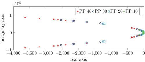
The frequency domain comparisons of the full and different dimensional reduced systems are shown in Figure 2 on the wide range 10¹–10⁴ [rad/s]. Figure 2(a) shows the frequency responses of full and reduced systems with good matching. The absolute error and the relative error of the frequency responses of full and reduced systems are exhibited in Figure 2(b,c), respectively. As we can see in Figure 2(c), the relative errors for all reduced systems are well below the truncation tolerance (10⁻⁵). We further compute the 40, 30, 20 and 10 dimensional ROMs using the same algorithm via balancing the system on the position–position level. In this case, the frequency responses of the reduced systems also resemble the graph in Figure 2(a). Figure 3 depicts the relative errors between the full and different dimensional ROMs. We observe that, as expected, the lower the dimension of the reduced models, the higher the relative error. But even a very low dimensional model, e.g. the model of dimension 10, preserves the important feature of the original model’s input/output behaviour, such that all of them are expected to work well as the basis of a high performance controller. Figure 4 shows that the ROM are all stable numerically as expected from the theory.

Figure 2. Comparison of original and different dimensional reduced systems (dimensions indicated in the legend) computed by Algorithm 2.

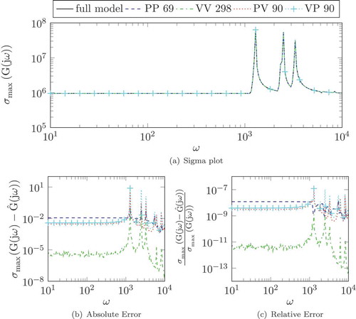
Figure 3. Relative error of full and different dimensional reduced systems (dimensions indicated in the legend) via balancing the system on the position level.

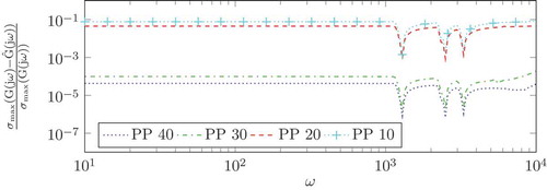
Figure 4. Eigenvalue structures of the different dimensional reduced models obtained by position–position balancing.

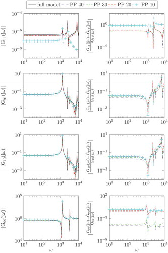
Figure 5 presents some particularly interesting SISO relations for full and different dimensional ROMs. We selected the exact same relations as in [1] for comparison with our earlier approaches. Since in the SISO case we know that the transfer function matrix is just a scalar rational function, here we have computed the absolute values of the transfer function in different frequencies. The relative errors between the original and ROMs of the respective SISO relation are also shown in the same figure. Comparing the results to the ones in [1], we see that using the new method, we can achieve a comparable error with models of almost half the dimension. Thus the new implementation is faster, requires less than half the memory during computations and, in contrast to the old method, guarantees stability of the ROM. Although we have observed stability in the old implementation as well, the new one is to be preferred due to all its advantages.

Figure 5. The rows respectively, show the 1st input (mechanical force) to 1st output (displacement), 9th input (electrical potential) to 1st output, 1st input to 9th output (charge) and 9th input to 9th output relations (left) and the respective relative errors (right) of full and reduced systems (dimensions indicated in the legend) for position–position balancing.

The acceleration we get from the exploitation of the block structure, i.e. the speedup of Algorithm 3 compared to Algorithm 1, are similar to the ones reported in [4,13]. Comparing the computation times of the new symmetry exploiting implementation with the one required to perform the general reduction approach reported in [1], we observe that the new version is roughly four times faster. The largest part of the time is spent computing the Gramian factors. A factor of about two is expected from the fact that here, we only need to compute one factor instead of two in the earlier approach. The real factor computation also only needs to solve one complex shifted linear system per pair of complex shifts instead of the two required before. This motivates a further factor of two, since in the vibrating system we investigate, most eigenvalues appear as complex pairs and, thus, so do the ADI shifts. In fact in our test, we observe a factor of 4.05 longer runtime for the previous implementation. Note that in both cases, we limited the number of ADI iterations to 100 in order to have a representative average per step timing and still fit both versions into the 48 GB RAM even with the suboptimal memory management experienced in MATLAB. The combined runtime for the computation of Gramian factors, projection matrices and reduced-order models was roughly 1 h and 15 min for the new symmetry exploiting case and 5 h and 6 min in the previous approach. We also observed that due to the improved shift selection, the convergence is often accelerated, especially in the index-1 case, see e.g. [20]. This can increase the speedup even further due to earlier termination of the Gramian factor computation.

If desired, an $\alpha$-shift strategy as proposed in [25] can be incorporated into both methods. This usually further accelerates convergence in the Gramian factor computation.

Additional details and numerical experiments can be found in [2, Chapter 2].

7. Conclusions

In this article, we have introduced an enhanced technique for structure preserving model reduction of a special class of second-order index-1 differential algebraic systems using balanced truncation. It is shown that the appropriate choice of the first-order representation of this type of systems enables us to solve one Lyapunov equation only, which reduces both computational cost and memory requirement by roughly one half. The Lyapunov equation is solved efficiently by using recent updates to the basic low-rank ADI iteration. We also have adapted the way to solve the linear system in each iteration step of the low-rank ADI method by exploiting the block structure. Compared to our earlier article [1], a different reformulation to first-order form was used. Similar to [1], we enable the optimal exploitation of the original matrices, which may dramatically decrease the computational cost. The performance of our proposed strategy has been demonstrated for one large FEM model of an ASS employing piezo actuators with almost 300,000 DoF, proving the applicability of our method in real world problems. In the numerical results, we have seen that even the 10 dimensional model nicely preserves the general behaviour of the transfer function of the original model in frequency domain. Therefore, it is expected to have a good performance in controller design. In [3], the authors showed that in general none of the existing BT techniques for second-order systems guarantees stability of the reduced systems. For the case of symmetric systems with collocated inputs and outputs, using our proposed method, stability can be guaranteed by Theorem 4.1, which is numerically depicted in Figure 4 and serves as the possibly most important advantage of the new method.

Acknowledgements

The authors express their thanks to Burkhard Kranz at the Fraunhofer Institute for machine tools and forming technology in Dresden (Germany) for providing the finite element model used in the numerical experiments.

M. Monir Uddin was also affiliated to the ‘International Max Planck Research School (IMPRS) for Advanced Methods in Process and System Engineering (Magdeburg)’.

The work of Peter Benner and Jens Saak has partially been supported by the collaborative research centre CRC/TR-96 of the Deutsche Forschungsgemeinschaft (DFG) within the subproject A06 ‘Model Order Reduction of Thermo-Elastic Assembly Group Models’.

Disclosure statement

No potential conflict of interest was reported by the authors.

Additional information

Funding

This work was supported by the Deutsche Forschungsgemeinschaft: [SFB/TR-96 TPA06].

References

- M.M. Uddin, J. Saak, B. Kranz, and P. Benner, Computation of a compact state space model for an adaptive spindle head configuration with piezo actuators using balanced truncation, Prod. Eng. 6 (2012), pp. 577–586. doi:10.1007/s11740-012-0410-x
- M.M. Uddin, Computational methods for model reduction of large-scale sparse structured descriptor systems, Ph.D. thesis, Otto-von-Guericke-Universität, Magdeburg, 2015. Available at http://nbn-resolving.de/urn:nbn:de:gbv:ma9:1-6535
- T. Reis and T. Stykel, Balanced truncation model reduction of second-order systems, Math. Comput. Model. Dyn. Syst. 14 (2008), pp. 391–406. doi:10.1080/13873950701844170
- P. Benner and J. Saak, Efficient balancing-based MOR for large-scale second-order systems, Math. Comput. Model. Dyn. Syst. 17 (2011), pp. 123–143. doi:10.1080/13873954.2010.540822
- Z. Bai and Y.F. Su, Dimension reduction of large-scale second-order dynamical systems via a second-order Arnoldi method, SIAM J. Sci. Comput. 26 (2005), pp. 1692–1709. doi:10.1137/040605552
- B. Salimbahrami and B. Lohmann, Order reduction of large scale second-order systems using Krylov subspace methods, Lin. Alg. Appl. 415 (2006), pp. 385–405. doi:10.1016/j.laa.2004.12.013
- P. Benner, J. Saak, and M.M. Uddin, Second order to second order balancing for index-1 vibrational systems, 7th International Conference on Electrical & Computer Engineering (ICECE) 2012, Pan Pacific Sonargaon, Dhaka, 2012, pp. 933–936.
- K. Glover, All optimal Hankel-norm approximations of linear multivariable systems and their L norms, Int. J. Control 39 (1984), pp. 1115–1193. doi:10.1080/00207178408933239
- M.S. Tombs and I. Postlethwaite, Truncated balanced realization of a stable nonminimal state-space system, Int. J. Control 46 (1987), pp. 1319–1330. doi:10.1080/00207178708933971
- P. Benner, J.-R. Li, and T. Penzl, Numerical solution of large-scale Lyapunov equations, Riccati equations, and linear-quadratic optimal control problems, Numer. Lin. Alg. Appl. 15 (2008), pp. 755–777. doi:10.1002/nla.v15:9
- T. Penzl, A cyclic low rank Smith method for large sparse Lyapunov equations, SIAM J. Sci. Comput. 21 (2000), pp. 1401–1418. doi:10.1137/S1064827598347666
- P. Benner, P. Kürschner, and J. Saak, Efficient handling of complex shift parameters in the low-rank Cholesky factor ADI method, Numer. Algorithms 62 (2013), pp. 225–251. doi:10.1007/s11075-012-9569-7
- P. Benner, P. Kürschner, and J. Saak, An improved numerical method for balanced truncation for symmetric second order systems, Math. Comput. Model. Dyn. Syst. 19 (2013), pp. 593–615. doi:10.1080/13873954.2013.794363
- W.-G. Drossel and V. Wittstock, Adaptive spindle support for improving machining operations, CIRP Ann. Manuf. Technol. 57 (2008), pp. 395–398. doi:10.1016/j.cirp.2008.03.051
- R. Neugebauer, W.-G. Drossel, A. Bucht, B. Kranz, and K. Pagel, Control design and experimental validation of an adaptive spindle support for enhanced cutting processes, CIRP Ann. Manuf. Technol. 59 (2010), pp. 373–376. doi:10.1016/j.cirp.2010.03.029
- R. Neugebauer, W.-G. Drossel, K. Pagel, and B. Kranz, Making of state space models of Piezo-mechanical systems with exact impedance mapping and strain output signals, Mechatronics and Material Technologies, June 28–30, Vol. 2, Swiss Federal Institute of Technology ETH, Zurich, 2010, pp. 73–80.
- D.G. Meyer and S. Srinivasan, Balancing and model reduction for second-order form linear systems, IEEE Trans. Autom. Control 41 (1996), pp. 1632–1644. doi:10.1109/9.544000
- Y. Chahlaoui, D. Lemonnier, A. Vandendorpe, and P.V. Dooren, Second-order balanced truncation, Lin. Alg. Appl. 415 (2006), pp. 373–384. doi:10.1016/j.laa.2004.03.032
- P. Benner and J. Saak, Numerical solution of large and sparse continuous time algebraic matrix Riccati and Lyapunov equations: a state of the art survey, GAMM Mitteilungen 36 (2013), pp. 32–52. doi:10.1002/gamm.v36.1
- P. Benner, P. Kürschner, and J. Saak, Self-generating and efficient shift parameters in ADI methods for large Lyapunov and Sylvester equations, Electron. Trans. Numer. Anal. 43 (2014), pp. 142–162.
- P. Benner and T. Stykel, Model order reduction for differential-algebraic equations: a survey, preprint MPIMD/15-19, Max Planck Institute Magdeburg (2015). Available at http://www.mpi-magdeburg.mpg.de/preprints/
- M. Marcus and H. Minc, A Survey of Matrix Theory and Matrix Inequalities, Allyn and Bacon, Boston, 1964.
- T.A. Davis, Direct Methods for Sparse Linear Systems, No. 2 in Fundamentals of Algorithms, SIAM, Philadelphia, 2006.
- Y. Saad, Iterative Methods for Sparse Linear Systems, SIAM, Philadelphia, 2003.
- F. Freitas, J. Rommes, and N. Martins, Gramian-based reduction method applied to large sparse power system descriptor models, IEEE Trans. Power Syst. 23 (2008), pp. 1258–1270. doi:10.1109/TPWRS.2008.926693
- B. Kranz, Zustandsraumbeschreibung von Piezo-mechanischen Systemen auf Grundlage einer Finite-Elemente-Diskretisierung, ANSYS Conference & 27th CADFEM Users’ Meeting, November 18–20, Congress Center Leipzig, Germany, 2009.
- M. Heinkenschloss, D.C. Sorensen, and K. Sun, Balanced truncation model reduction for a class of descriptor systems with application to the Oseen equations, SIAM J. Sci. Comput. 30 (2008), pp. 1038–1063. doi:10.1137/070681910