Modelling and simulation of self-regulating pneumatic valves

ABSTRACT

In conventional aircraft energy systems, self-regulating pneumatic valves (SRPVs) are used to control the pressure and mass flow of the bleed air. The dynamic behaviour of these valves is complex and dependent on several physical phenomena. In some cases, limit cycles can occur, deteriorating performance. This article presents a complex multi-physical model of SRPVs implemented in Modelica. First, the working principle is explained, and common challenges in control-system design-problems related to these valves are illustrated. Then, a Modelica-model is presented in detail, taking into account several physical domains. It is shown, how limit cycle oscillations occurring in aircraft energy systems can be reproduced with this model. The sensitivity of the model regarding both solver options and physical parameters is investigated.

KEYWORDS:

• Modelica
• thermofluid
• modeling
• friction
• electrohydraulic
• hydraulic

1. Introduction

In applications related to process control often relatively simple valve models are used. They are based on flow coefficients, and relate mass flow to pressure drop by the use of a quadratic relationship. This helps keeping the system model at a low order, benefitting understanding as well as control design. Most of the time, these simple models are accurate enough.

There are, however, applications where simple models are inadequate. This can be the case if high accuracy is needed, when choking occurs, or when internal valve phenomena are relevant. Neglecting these cases can lead to unwanted behaviour in the controlled system: internal valve dynamics often contain nonlinearities like stiction, backlash and deadband, which in turn can lead to oscillations [2].

Indeed, according to Bialowski [3], about 30% of controlled loops in the process industry are oscillating. In Desborough and Miller [4], 26,000 PID controllers in the process industry are surveyed: 16% are classified as excellent, 16% as acceptable, 22% as fair, 10% as poor, and 36% run in open-loop.

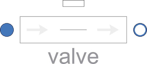
In aircraft, self-regulating pneumatic valves (SRPVs) are used to control the pressure and flow rate of the engine bleed air. An illustration of the working principle can be found in Figure 1, more detailed descriptions can be found in Section 2.

Figure 1. Illustration of a self-regulating pneumatic valve.

SRPVs operate under harsh conditions inside the engine nacelle. Since several SRPVs are operated in-line, their dynamic behaviour has to be tuned so as to avoid the occurrence of limit cycles. This can be done in situ, but the associated costs are substantial. Being able to predict the system behaviour better during the design phase would reduce those costs considerably, but for a sufficient level of prediction-accuracy a high-fidelity model is needed.

Related research has been done by several authors. In Beater [5], a simple model of an electro-hydraulic valve in Modelica and HyLib is presented. In Beater and Clauß [6], a pneumatic drive system is modelled in Modelica, combining pneumatic, mechanical and electronic domains. A free-piston-engine modelled in Modelica is described in Pohl and Gräf [7], containing detailed submodels of several physical domains. In Pujana-Arrese et al. [8], a Modelica-model of a pneumatic muscle is presented, combining fluid with mechanical modelling.

The goal of this article is to demonstrate how high-fidelity multi-physical models of self-regulating pneumatic valves can be developed in the object-oriented equation-based modelling-language Modelica, and how oscillations occuring in real-life industrial applications can be reproduced. It is structured as follows: In Section 2, the Modelica model for SRPVs is presented and the motivations for modelling choices are explained, subdivided into the different physical domains. Libraries, models and implementations used in this work are mentioned. In Section 3, it is demonstrated how valve oscillations occuring in aircraft energy systems can be reproduced with this model. In Section 4, a roadmap for the controller design of self-regulating pneumatic valves is laid out. In Section 5, the sensitivity of simulation results to several solver- and physical parameters is investigated. In Section 6, interesting interaction-effects between the different physical domains are shown and corresponding simulation results are presented. The article is concluded in Section 7.

2. Valve modelling

2.1. Functioning principle

The main functioning principle of a self-regulating pneumatic valve is based on automatic pressure balancing. A small pipe connects the main pipe downstream of the valve with the lower end of the valve actuator chamber. The hydraulic resistance of this pipe dominates the time constant of the valve dynamics, its diameter is therefore an important design parameter. Inside the chamber, a piston divides the chamber into two volumes.

The piston is connected to the butterfly valve disc by a mechanical link. In this way, if the downstream pressure increases, the pressure in the lower part of the chamber increases as well and moves the piston upwards. This closes the valve disc, leading to a lower valve mass flow. Depending on the flow configuration in the remainder of the circuit, this usually decreases the downstream pressure, closing the feedback loop.

Additionally, a second control loop is present. By the use of pressure-reducers, vents, and/or small electric regulating valves, air can flow from the upstream part of the pipe to the upper chamber, or from the upper chamber to the ambient. The implementation of the second loop can differ by a great deal, in this work two implementations are modelled:

1. pneumatic actuator: a pneumatic system using two pressure-reducers keeps the pressure in the upper chamber inside a predefined interval

2. electro-pneumatic actuator: a PID-controller directly imposes the air mass-flow from or into the upper chamber

For the sake of clarity, the top-level model of the self-regulating pneumatic valve has been split into two parts: one valve-part and one actuator-part. The partitioning is illustrated in Figure 1, where the valve part is depicted in dashed-grey lines.

2.2. Detailed valve model

The valve model calculates the mass flow through the valve depending on the up- and downstream fluid properties and the valve angle. The symbol and the connectors of the valve model are depicted in Figure 2. One (rectangular) mechanical multi-body connector is used to connect the valve disc with the valve actuator. Two (round) fluid-connectors are used to connect the valve to pipe models upstream and downstream.

Figure 2. Modelica symbol layer of the valve model.

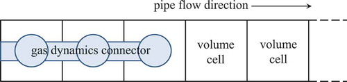
In aircraft bleed air systems, flow velocity is quite high. Physical effects of high-speed compressible flow cannot be neglected [9], so the capabilities of the Modelica Fluid library are not sufficient. Thus, as fluid interface, higher-order stencil-based connectors for gas-dynamics as presented in Sielemann [10] are used. These connectors include far more information than the connectors from the Modelica Fluid library: for a variable number of fluid cells, pressure, temperature and fluid velocity are included. This is illustrated in Figure 3. With this information, higher order discretization schemes of computational fluid dynamics can be used.

Figure 3. Illustration of the gas-dynamics connector principle, including information about multiple volume cells.

The numerical scheme to compute the desired variables was chosen based on several numerical experiments. We chose a Godunov-type scheme, Roe monotone flux [11], for its combination of robustness, accuracy and performance.

For the mass flow calculation choked flow effects can occur and have to be taken into account. Therefore the standard calculation using flow coefficients is discarded. Instead, a flow function approach is used, based on an enthalpy-balance and adiabatic state change. The corresponding equations are shown in Equation (1). Note that the flow calculation is symmetric in regard to flow direction. This is not completely accurate, but since the valve is used as a pressure-reducer, back-flow cases are only hypothetically relevant. The result of this function is multiplied by a factor that is dependent on the valve angle:

(1) $\begin{array}{rl}& rati{o}_{\mathrm{c}\mathrm{r}\mathrm{i}\mathrm{t}}=(\frac{2}{\kappa +1}{)}^{\frac{\kappa }{\kappa -1}}\\ & p_{\mathrm{m}\mathrm{a}\mathrm{x}}=\mathrm{m}\mathrm{a}\mathrm{x}(p_{\mathrm{u}\mathrm{p}\mathrm{s}\mathrm{t}\mathrm{r}\mathrm{e}\mathrm{a}\mathrm{m}},p_{\mathrm{d}\mathrm{o}\mathrm{w}\mathrm{n}\mathrm{s}\mathrm{t}\mathrm{r}\mathrm{e}\mathrm{a}\mathrm{m}})\\ & p_{\mathrm{m}\mathrm{i}\mathrm{n}}=\mathrm{m}\mathrm{i}\mathrm{n}(p_{\mathrm{u}\mathrm{p}\mathrm{s}\mathrm{t}\mathrm{r}\mathrm{e}\mathrm{a}\mathrm{m}},p_{\mathrm{d}\mathrm{o}\mathrm{w}\mathrm{n}\mathrm{s}\mathrm{t}\mathrm{r}\mathrm{e}\mathrm{a}\mathrm{m}})\\ & ratio=p_{\mathrm{m}\mathrm{i}\mathrm{n}}/p_{\mathrm{m}\mathrm{a}\mathrm{x}}\\ & \psi =\left(\begin{array}{cc}{(\frac{2}{\kappa +1})}^{\frac{1}{\kappa -1}}{(\frac{\kappa }{\kappa +1})}^{\frac{1}{2}}& \mathrm{i}\mathrm{f}ratio<rati{o}_{\mathrm{c}\mathrm{r}\mathrm{i}\mathrm{t}}\\ \sqrt{\frac{\kappa }{\kappa -1}rati{o}^{\frac{1}{\kappa }}(rati{o}^{\frac{1}{\kappa }}-ratio)}& \mathrm{i}\mathrm{f}1>ratio>rati{o}_{\mathrm{c}\mathrm{r}\mathrm{i}\mathrm{t}}\\ \hspace{0.17em}& \hspace{0.17em}\end{array}\right. \\ & m_{\mathrm{f}\mathrm{l}\mathrm{o}\mathrm{w}}=\psi area\sqrt{{\rho }_{\mathrm{u}\mathrm{p}\mathrm{s}\mathrm{t}\mathrm{r}\mathrm{e}\mathrm{a}\mathrm{m}}2p_{\mathrm{m}\mathrm{a}\mathrm{x}}}\end{array}.$(1)

Fluids moving through a butterfly valve at high velocities induce a fluiddynamic torque on the valve disc. This generates an interesting coupling between the fluid and mechanic domains of a valve model. For the calculation of the torque, two approaches are often used: one based on the pressure difference, one based on the fluid velocity. In Solliec and Danbon [12], the different approaches are compared. We use the classical approach based on pressure difference, as the pressure difference is more clearly defined than the fluid velocity in the context of lumped parameter models. Here, the torque T is calculated as

(2) $T(\alpha )=K(\alpha )\mathrm{\Delta }P{D}^3,$(2)

where K is the torque coefficient, $\mathrm{\Delta }P$ is the pressure difference, $\alpha$ is the valve angle and D is the valve diameter. A spline-based approach is used to describe the dependency between torque coefficient and valve angle. This data can be generated either from computational fluid dynamics (CFD)-calculations, measurements or vendor data. A Modelica multibody connector provides the valve angle and feeds back the induced fluiddynamic torque.

2.3. Actuator model

Two actuator models, as described in Section 2.1, are needed, for two different implementations of the second control loop. Accordingly, one partial model together with two extending models was created. The Modelica diagram of the purely pneumatic version can be seen in Figure 4.

Figure 4. Modelica component layer of the pneumatic valve actuator model.

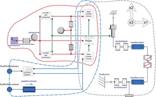
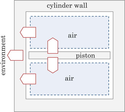
Three physical domains are significant for the modelling of the valve actuator: the fluid dynamics inside the chambers, the multi-body mechanics of the mechanism, and the thermal behaviour of the parts. They are connected through the piston and chamber components, where all domains have considerable influence. The domains are indicated in Figure 4 through colored lines: dashed-grey indicates the mechanical domain, dotted-red indicates the thermal domain, and dashed-dotted blue indicates the fluid domain.

2.3.1. Mechanical domain

The core of the mechanical domain is the piston-model, where a one-dimensional force balance over the piston is calculated (see Equation (3)). The occurring forces are commented in the following:

(3) $\begin{array}{rl}& F_{\mathrm{p}\mathrm{r}\mathrm{e}\mathrm{s}\mathrm{s}\mathrm{u}\mathrm{r}{\mathrm{e}}_{\mathrm{u}\mathrm{p}\mathrm{p}\mathrm{e}\mathrm{r}}}+F_{\mathrm{p}\mathrm{r}\mathrm{e}\mathrm{s}\mathrm{s}\mathrm{u}\mathrm{r}{\mathrm{e}}_{\mathrm{l}\mathrm{o}\mathrm{w}\mathrm{e}\mathrm{r}}}+F_{\mathrm{c}\mathrm{o}\mathrm{n}\mathrm{s}\mathrm{t}\mathrm{r}\mathrm{a}\mathrm{i}\mathrm{n}\mathrm{t}}\\ & +F_{\mathrm{f}\mathrm{r}\mathrm{i}\mathrm{c}\mathrm{t}\mathrm{i}\mathrm{o}\mathrm{n}}+F_{{\mathrm{d}}^{\prime }\mathrm{A}\mathrm{l}\mathrm{e}\mathrm{m}\mathrm{b}\mathrm{e}\mathrm{r}\mathrm{t}}+F_{\mathrm{j}\mathrm{o}\mathrm{i}\mathrm{n}\mathrm{t}}=0\end{array}.$(3)

• Pressure forces

The piston model and both chamber models are connected by translational mechanical connectors. In this way, the position and the forces generated by fluid pressure are exchanged.

• Constraining forces

Based on the construction, the movement allowance of the piston is limited. To represent this, stiff quadratic spring forces are implemented. These come into effect as soon as the end of the stroke is reached.

• Friction forces

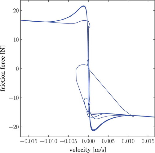
The friction forces between piston and cylinder are mainly responsible for unwanted stiction effects. Detailed modelling of friction phenomena is, therefore, necessary. Furthermore, a simple model based on two static and dynamic friction coefficients is numerically unfavourable when the piston position is used as a state. In this work, we used the Lund–Grenoble (Lu–Gre) friction model [13]. It is a detailed model of friction with an internal state that represents the deflection of the bristles (micro-bumps in the material surface). The implementation in Modelica was done according to Aberger and Otter [14], but instead of rotational coordinates, translational coordinates were used. An example of the trajectory of the friction force over piston velocity can be seen in Figure 5.

• d’Alembert force

Figure 5. A trajectory (friction force w.r.t. velocity) of the Lund–Grenoble friction model.

The d’Alembert force, or inertial force, of the piston is calculated by deriving the position w.r.t. time two times and multiplying it by its mass. Of course, this makes the system quite stiff from a numerical point of view, but then, there are solvers of production-quality available to handle stiff systems.

• Joint force

The joint force is the linking force between the translational piston dynamics and the planar dynamics of the mechanism. The prismatic joint model of the multibody library provides the interface.

For the dynamics of the mechanism, the Modelica Multibody library as presented in Otter et al. [15] is used. With this library, the mechanism can be represented exactly; also an extension to alternative designs can be done with little effort. Unfortunately, a nonlinear system of equations remains after causalization of the complete model.

2.3.2. Fluid domain

For the air in the valve actuator, high-speed fluid effects can be neglected. Consequently, the Modelica fluid library as presented in Casella et al. [16] is used wherever possible.

Both valve chambers correlate to variable volume models. The governing equations of a variable volume model are a generalization of the standard volume model equations, and take the form of Equation (4), with the density $\rho$, the volume V, and $\varphi \in (1,u,\mathbf{x})$ representing mass, energy and substance balance, respectively.

(4) $\frac{\mathrm{d}}{\mathrm{d}t}(\varphi \rho V)={\sum }^{f}low+{\sum }^{s}ource.$(4)

In the case of the energy-balance, mechanical work on the cylindrical chamber volume now creates an interesting interaction between the fluid and mechanical domain. The implementation in Modelica can be seen in Listing 1. Note: the actualStream-operator indicates the properties of the fluid crossing the port boundary. The noEvent-operator indicates that no state-events shall be generated when the fluid mass flow changes direction.

1. Listing 1. Extract of Modelica code for lower variable volume model

//translational mechanics interface

medium . p = - flange. f/area ;

pos = flange . s ;

volume = volume_0 + area * pos;

//mass balance

mass = volume * medium . d ;

der(volume * medium . d) = sum(fluidPort . m_flow) ;

//energy balance (Du = dQ + dW)

der(volume*medium . d * medium . u) = sum(fluidPort[i] . m_flow *noEvent(actualStream(fluidPort[i] . h_outflow)) for i in 1:ninf)- medium . p * der(volume) + heatPort . Q_flow ;

//substance balance

der(volume * medium . d * medium . Xi) = sum(fluidPort[i] . m_flow * noEvent (actualStream(fluidPort[i] . Xi_outflow)) for i in 1 : ninf) .

2.3.3. Thermal domain

The thermal effects in self-regulating pneumatic valve systems are largely dominated by the advection in the air. This is obviously already included in the fluid modelling. Nonetheless, conduction through the solid components still has to be modelled if high-fidelity results are necessary.

On the thermal side, the model is structured as follows. The environment is modelled as boundary condition of constant temperature. The actuator cylinder wall and piston are both modelled as thermal masses. A further discretization is discarded based on the high internal conductivity of the used materials. The energy dissipated by friction is added to the piston wall. Between the fluid volumes and the piston mass, as well as between the cylinder wall and the environment, constant thermal conductances are assumed. Between the fluid volumes and the cylinder wall, the thermal conductance is dependent on the wetted area, which is in turn dependent on the piston position.

As a consequence, a heat-conduction component was composed that connects heat conductivity with the piston position. The remainder was modelled using the Modelica thermal heat transfer library, the details of which are described by Tiller [17].

In Figure 6, the structure of the thermal model is illustrated.

Figure 6. Thermal structure of the valve actuator.

2.4. Statistics

Before simulation, the previously acausal model is causalized and index-reduction takes place wherever necessary (for more details see [18]). The resulting models of valve and actuator features 0 and 10 states respectively, and 21 and 161 time-varying variables. After tearing, a nonlinear system of size 3 remains for the actuator model, caused by the multibody mechanics.

3. Limit cycle oscillations

For reasons of confidentiality, no real-life, industrial valve setups or associated measurements can be presented here. Instead, a simpler composition is shown, where two valves are used to reduce the pressure in a pipe. The Modelica diagram of the composition can be seen in Figure 7. The pipe models are based on the gas dynamics library as presented by [10]. Each pipe-component represents a pipe of 20 m length and a diameter of 0.1 m, totalling at a length of 80 m and a volume of around 0.63 m³.

Figure 7. Modelica diagram of oscillation test case.

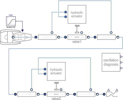
As boundary conditions, the input pressure (left side) is set to 3 bars, while the right boundary is modelled as a quadratic resistance, normalized to a fluid velocity of 10 m/s $\frac{m}{s}$ at a pressure of 1 bar. The valve actuators are run in pneumatic-mode and set to regulate the downstream pressure to 2 and 1 bars, respectively.

When the composite model is simulated, limit cycle oscillations occur. These are displayed in Figure 8. For both valves, the piston gets stuck at the outmost deflection, until the restoring forces are high enough to overcome the friction forces.

Figure 8. Results of oscillation test case.

To demonstrate the influence of friction and pneumatic forces on the oscillations, the friction force and the volume of the cylinders were multiplied with a scaling parameter. A two-dimensional sweep of the quasi-steady-state amplitudes and periods over both scaling-parameters is shown in Figure 9.

Figure 9. Amplitude and period of oscillations for scaled friction forces and cylinder volumes.

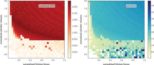
It can be seen that the oscillations are strongly dependent on both factors. Furthermore, the interaction between both factors can be visibly divided into three sections: for friction forces or cylinder volumes below a certain treshold, no oscillation takes place, no matter how large the other scaling factor is. As long as both factors are relatively small, some interactions can be seen.

4. Modelling and control system design

4.1. Introduction

The Modelica technology allows for an integrated development of both plant model and control system. In the case at hand, control of electro-pneumatic valves is a difficult task: As demonstrated in Section 3, or in works like [19], valve oscillations are mainly dominated by friction forces. This phenomenon is usually called stiction, a combination of the words ‘stick’ and ‘friction’. The balancing of stiction with the tools of control systems engineering is called ‘stiction compensation’.

In literature, two main strategies are described regarding stiction compensation. The first strategy (the knocker) uses pulses of predefined length and intensity on top of the regular control signal to overcome the stiction regime [20]. The other (dithering) superimposes the control signal with a high-frequency zero-mean signal to average-out the friction characteristic [21]. For self-regulating pneumatic valves both approaches are not suitable: the control signal has no direct influence on the valve stem, instead it imposes a mass flow on one of the valve chambers. In this way, the control signal is first-order filtered. Conventional stiction compensation strategies require a high-frequency interaction between actuator and valve stem, which is, therefore, not possible.

4.2. Control-driven modelling

In this work, we propose an alternative workflow, which is tied into the modelling aspect of the controlled system. The main idea is to use the detailed model to find the best combination of sensors and sensor-positions to robustly estimate the current friction force during the valve operation. Knowledge about the current friction force can in turn be used to compensate for stiction-effects.

The complete workflow is summarized in Figure 10 and executed as follows:

• Modelling of valve without friction

Figure 10. Control system development strategy.

From the complete actuator model, the friction force is multiplied by zero. Alternatively, the damping term $F_{v}v$ can remain, if necessary for stability.

• Modelling of external controller interface

Normally, autonomous models are used. To change this, the actuator model is extended with an external input, governing the mass flow into the upper cylinder. Additionally, relevant measurements are output.

• Build-up of simple system model

Using frictionless valve models with external interfaces, the complete system is modelled. Low-order pipe models are preferable, if analytic control design approaches like linear quadratic gaussian control are to be used later.

• Linearization of system model around set-point

The system model is simulated until a steady state is reached. Using the linear systems as described in Baur et al. [22], the system is linearized and the resulting state-space representation is exported.

• Development of a controller for linearized model

Using standard approaches like LQG or $H_{\mathrm{\infty }}$, a MIMO-controller for the resulting system is designed.

• Testing of controller on detailed model without friction

The controller is tested on a the system model in Modelica. If the performance is not satisfactory, another controller has to be designed.

• Development of friction estimator

During the sticking-phase of the valve operation, the piston does not move but the friction force does change over time. This force itself is not directly measurable, but it can be estimated. Based on prior knowledge about which variables can be measured, different estimators can be developed and compared inside the modelling context. Key for this estimation is the force balance over the piston as described in Equation (3), where all terms apart from the friction term can be measured, calculated or are small during normal operation. The friction is then estimated as the missing term that brings the sum of forces to zero.

• Development of friction compensator

As soon as a suitable estimator is available, information about the current friction force during operation can be used to design a friction compensator. Since the friction force can now be considered in an isolated way, a relatively high gain can be used to offset this force without compromising system level stability. Another approach could be implemented by augmenting the input of the integral action of the main controller with an offset based on the estimated friction, alleviating a common cause of limit cycle oscillations at the cost of a non-zero steady-state error. The detailed development of friction compensation schemes goes beyond the scope of this article.

• Integration of compensator into controller

On the system level, a friction compensator is integrated into the MIMO-controller for each valve inside the system.

• Testing of compensated controller on detailed model

The complete system including friction is tested, using the compensated MIMO-controller. If the performance is not satisfactory, another approach for friction compensation has to be used.

5. Model sensitivities

In this section, the sensitivity of simulation results is analysed. First, a suitable test setup is presented. Then, the effect of physical parameters and solver options on the results of this test model is presented.

5.1. Test model

During model testing, it became apparent that the valve dynamics can be classified into three categories, depending on the boundary conditions and parameterization of the valve.

1. In some cases, the overall dynamics were stable, which resulted in a steady-state system as soon as initialization effects died down.

2. In some cases, the system showed a chaotic behaviour.

3. In the other cases, the system dynamics exhibited stable limit cycles.

To find a quantifiable metric for model sensitivities, steady-state cases are not interesting, while chaotic cases make it difficult to quantify model differences. Therefore, we chose a setup including limit-cycles as test-case. Accordingly, the model from Section 3 was used. It was simulated for 25 s and the final frequency and amplitude of the output pressure of the first valve were used as a comparison-variable.

5.2. Solver options

Reasonable solver settings can be suggested by the following simple heuristic: the test model is simulated using a large solver tolerance and the values of oscillation amplitude and frequency are stored. The solver tolerance is then reduced and the simulation is repeated. This continues until the values of oscillation amplitude and frequency do not change anymore. The largest tolerance that results in this final values is defined as the required solver tolerance.

We tested the following solvers: lsodar, dassl,¹ runge-kutta4, radau2a, esdirk23a, dopri45, sdirk34hw, cerk23 and cvode. As the model is quite stiff due to the friction dynamics, only four of those were able to solve the system in an acceptable time span. Those four (dassl, sdirk34hw, lsodar, cvode) were analysed as described. The results can be seen in Figure 11.

Figure 11. Sensitivities of solver parameters.

Evidently, the required solver tolerance is smallest for cvode (1e–5) and largest for dassl (3e–3). The required solver tolerance is the tolerance where the predicted amplitude matches the asymptotic amplitude. However, using all four solvers at their respective required tolerance values, cvode is still the fastest.

One definition of model stiffness is the following: ‘A model is stiff if the simulation requires stiff solvers’. In that sense, the model is stiff, since all adequate solvers (dassl, sdirk34hw, lsodar, cvode) are as well.

5.3. Physical parameters

To use the model for simulations, a set of physical parameters has to be defined. Most of them have a geometrical meaning and can simply be looked up from the specifications. For accurate results, there are however three separate measurements to be done. In the following sections, the necessary measurements are introduced and the sensitivity of simulation results to those parameters is investigated. From those findings, suggestions regarding the necessary exactness of model parameters are made.

5.4. Friction

In the calculation of the piston-friction as appearing in Equation (3), the Lu–Gre friction model [13] is used. In this model, the friction characteristics are defined by 6 constants. These have to be looked up in literature, based on the material-pairing, or obtained from experiments if exact results are needed.

For each of those six parameters, we sweeped the parameter values one-by-one and simulated the test model. All other parameters where fixed. The resulting values for oscillation amplitude and frequency can be seen in Figure 12.

Figure 12. Sensitivities of friction parameters (reference values are marked).

Obviously, it is not easy to interpret this figure. The highly nonlinear friction model introduces chaotic behaviour into the system. This results in significant model differences even for negligible parameter deviations.

However, it is still possible to derive meaningful conclusions from this data: the first two parameters, $F_s$ and $F_c$, correspond to the static and sliding friction forces in simpler friction models. It can be seen that the oscillation amplitude increases with $F_s$ (the static friction) and decreases with $F_c$ (the sliding friction). This makes sense physically, as a large difference between both values increases the stick-slip effect, which is the main reason for valve oscillations.

The second two parameters, $v_s$ and $F_v$, exhibit a treshold behaviour, where the oscillations vanish for $v_s>0.0038\mathrm{m}/\mathrm{s}$ or $F_v<90\mathrm{N}\mathrm{s}/\mathrm{m}$. It is of course strongly recommended to repeat this analysis after measuring friction parameters, to see if the treshold values are near the measured values. If so, the validity of the model will be questionable. Apart from this treshold effect, the influence of $F_v$ seems to be small, while $v_s$ exhibits a medium influence on the resulting oscillations.

The last two parameters, ${\sigma }_0$ and ${\sigma }_1$, have a medium and low influence on the oscillations, respectively.

In summary, when using this model, accurate measurements should be applied for the derivation of the friction parameters. ${\sigma }_1$ seems to be the least important factor, while $F_v$ only plays an important role if the value is near a certain treshold.

5.5. Aerodynamic torque

The aerodynamic torque as described in Equation (2) is a function on the angle of the valve-disc. This function differs somewhat based on the geometry, but can often be estimated by CFD calculations.

In this analysis, we modelled the effects of dimension as well as shape deviations of this function.

To get a feel for the influence of the dimension on the oscillation dynamics, we multiplied the computed torque with a scaling parameter. The result of a parameter sweep can be seen in Figure 13.

Figure 13. Sensitivity of aerodynamic forces.

Of course, not only the absolute factor of the aerodynamic torque can influence the system dynamics, but also the shape of the valve angle-dependency. To analyse this, we extended the torque calculation with the term $(1+scaleaero\ast \mathrm{s}\mathrm{i}\mathrm{n}(Angle\ast 3\ast \pi /90))$, resulting in an angle-dependent deviation. The resulting functions can be seen in Figure 14 for values of the scaling parameter scaleaero of −0.2 and 0.2. The function for a vanishing value of the scaleaero is shown in black as a reference.

Figure 14. Deviations in the aerodynamic torque as a function of the valve angle.

The result of a parameter sweep can be seen in Figure 15.

Figure 15. Sensitivity of the parameter scaleaero on aerodynamic forces.

To summarize, both deviations in dimension and in the shape of the valve angle-dependency can have a large influence on the resulting dynamics if the measured values are far off the actual values. However, one has to keep in mind that systematic errors will be introduced much more easily, while the shape of the valve angle-dependency will stay roughly the same, if measured. Therefore, the absolute factor seems to be far more important relatively. For most applications, it might be enough to take the values from literature, and scale the resulting function by the use of a single experiment.

5.6. Mass flow characteristic

Butterfly valves feature an S-shaped dependency between mass flow and valve angle. Like the aerodynamic torque, this dependency is not consistent between different valve-models. Therefore, CFD-calculations or experiments have to be deployed.

In the same schema as before, the effects of both dimension and shape deviations on the system oscillations were analysed. The results are presented in Figure 16.

Figure 16. Sensitivity of mass flow characteristic.

For both dimensional and shape variations, a treshold-effect is apparent. Even for small deviations in the wrong directions, the oscillations disappear instantly. This large sensitivity points to a great accuracy which is needed during the measurement of this curves.

6. Dynamic interactions

The multi-domain nature of the presented model results in some interesting nonlinear transients. Two of them are presented in the following.

6.1. Aerodynamic torque

The waterhammer effect is commonly known in pipeline operations. When a closing valve is used to stop the flow of a heavy and fast fluid-mass, the residual momentum of the fluid generates a build-up of pressure upstream of the valve.

For self-regulating pneumatic valves, a similar effect can occur: let’s presuppose that the valve actuator closes the valve by a particular angle. The air mass upstream of the valve is then decelerated as a result, while generating a temporary pressure build-up. This pressure-buildup in turn increases the aerodynamic torque on the valve disc, closing the disc further and amplifying the effect.

In Figure 17, a test model is represented where a pressure-regulated pipe is subjected to a harmonic inlet pressure with increasing frequency. The model was simulated with and without consideration of aerodynamic torque. The result of the simulation can be seen in Figure 18. It is easily recognizable that the valve opening is smaller when taking aerodynamic torque in consideration, especially at the frequencies that occur between 10 and 15 s.

Figure 17. Aerodynamic torque test model.

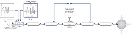
Figure 18. Transient effects of aerodynamic torque.

6.2. Oscillatory heating

Generally, the environment of the valve has an ambient temperature different from the fluid temperature in the pipe. In a typical application area, aircraft bleed air systems, the temperature difference can be around 500 K. Also, heat conduction between environment and the valve chambers takes place. In the static case, the temperature in the valve chamber will approach the ambient temperature after a time. However, in the case of valve movement, fluid mass is exchanged between the valve chambers and the pipe. In this way, the resulting temperature of the valve is dependent on the amount of valve movement.

In Figure 19, the same test model as presented in Figure 17 is subjected to a constant inlet pressure for 100 s, then subjected to an inlet pressure oscillating with a constant amplitude of 20 bars. The fluid inlet temperature is 500 K, and the environment temperature is 370 K. The inlet pressure oscillation results in significant valve movements, and therefore a significant increase in air temperature inside the cylinder volumes.

Figure 19. Transient effects of oscillatory heating.

7. Conclusion

Self-regulating pneumatic valves show a complex behaviour, resulting in limit-cycle oscillations, if the overall system is not tuned satisfactorily. We present a detailed Modelica model for this kind of valves. The model includes all relevant physical effects, representing the thermal, fluid, and mechanical domains. Simulation results exhibit the typical dynamical characteristics of self-regulating pneumatic valves. Subsequently, the model can be used to predict system performance in an early development phase.

Disclosure statement

No potential conflict of interest was reported by the authors.

Notes

1. Dassl is a native DAE-solver, but we used dassl as a regular ODE-solver, after preparing the equations as described in Section 2.4.

References

- A. Pollok and F. Casella, High-fidelity modelling of self-regulating pneumatic valves, Proceedings of the 11th International Modelica Conference, The International Federation of Automatic Control, Laxenburg, 2015.
- M.S. Choudhury, S.L. Shah, N.F. Thornhill, and D.S. Shook, Automatic detection and quantification of stiction in control valves, Control Eng. Pract 14 (2006), pp. 1395–1412. doi:10.1016/j.conengprac.2005.10.003
- W. Bialowski, Dreams vs. reality: a view from both sides of the gap, Pulp and Paper Canada. 94 (1993), pp. 19–27.
- L. Desborough and R. Miller, Increasing customer value of industrial control performance monitoring-Honeywell’s experience, AIChE symposium series, American Institute of Chemical Engineers, New York, 2002, pp. 169–189.
- P. Beater, Modeling and digital simulation of hydraulic systems in design and engineering education using Modelica and HyLib, Modelica workshop, Modelica Association, Linköping, 2000, pp. 23–24.
- P. Beater and C. Clauß, Multidomain systems: pneumatic, electronic and mechanical subsystems of a pneumatic drive modelled with modelica, Paper presented at the 3rd International Modelica Conference, Modelica Association, Linköping, 2003.
- S.E. Pohl and M. Gräf, Dynamic Simulation of a Free-piston Linear Alternator in Modelica, Proceedings of the 4th International Modelica Conference, Hamburg, March 7-8, Modelica Association, Linköping, 2005.
- A. Pujana-Arrese, J. Arenas, I. Retolaza, A. Martinez-Esnaola, and J. Landaluze, Modelling in Modelica of a pneumatic muscle: application to model an experimental set-up, 21st European Conference on Modelling and Simulation ECMS 2007, European Council for Modelling and Simulation, Pontypridd, 2007, pp. 4–6.
- M. Sielemann, Device-oriented modeling and simulation in aircraft energy systems design, Ph.D. diss., Hamburg University of Technology, 2012.
- M. Sielemann, High-speed compressible flow and gas dynamics, Proceedings of the 9th International Modelica Conference, Modelica Association, Linköping, 2012.
- P.L. Roe, Approximate riemann solvers, parameter vectors, and difference schemes, J. Comput. Phys 43 (1981), pp. 357–372. doi:10.1016/0021-9991(81)90128-5
- C. Solliec and F. Danbon, Aerodynamic torque acting on a butterfly valve. comparison and choice of a torque coefficient, J. Fluids. Eng 121 (1999), pp. 914–917. doi:10.1115/1.2823555
- C.C. De Wit, H. Olsson, K.J. Astrom, and P. Lischinsky, A new model for control of systems with friction, IEEE Trans on Auto Cont. 40 (1995), pp. 419–425.
- M. Aberger and M. Otter, Modeling friction in Modelica with the Lund-Grenoble friction model, Proceedings of the 2nd International Modelica Conference, Modelica Association, Linköping, 2002.
- M. Otter, H. Elmqvist, and S.E. Mattsson, The new modelica multibody library, Proceedings of the 3rd International Modelica Conference, Modelica Association, Linköping, 2003.
- F. Casella, M. Otter, K. Proelss, C. Richter, and H. Tummescheit, The Modelica Fluid and Media library for modeling of incompressible and compressible thermo-fluid pipe networks, Proceedings of the Modelica Conference, Modelica Association, Linköping, 2006, pp. 631–640.
- M. Tiller, Introduction to Physical Modeling with Modelica, Springer Science Business Media, Luxemburg, 2001.
- F.E. Cellier and E. Kofman, Continuous System Simulation, Springer Science & Business Media, Luxemburg, 2006.
- M.S. Choudhury, N.F. Thornhill, and S.L. Shah, Modelling valve stiction, Control. Eng. Pract 13 (2005), pp. 641–658. doi:10.1016/j.conengprac.2004.05.005
- T. Hägglund, A friction compensator for pneumatic control valves, J. Process. Control 12 (2002), pp. 897–904. doi:10.1016/S0959-1524(02)00015-X
- K.J. Åström, Control of Systems with Friction, Swedish. The Fourth International Conference on Motion and Vibration Control, ETH Zürich, Zürich, 1998.
- M. Baur, M. Otter, and B. Thiele, Modelica libraries for linear control systems, Proceedings of 7th International Modelica Conference, Como, Italy, September, Modelica Association, Linköping, 2009, pp. 20–22.