Automated safety analysis by minimal path set detection for multi-domain object-oriented models

ABSTRACT

A method called DMP for Detection of the Minimal Path set of any fault-tolerant technical system, the system being represented as a multi-domain object-oriented model, is described, exemplified and substantiated in this article. Thus, by use of DMP, a safety analysis of the system is automatically performed. DMP employs simulation of normal behaviour, degradation and failure of a system. In essence, it is a state space simulation. The state space, in this context, denotes the set of combinations of intact and failed components of a system to be examined for detection of its minimal path set. Without any reduction technique, the size of a system’s state space grows exponentially with the number of its components. In order to render the DMP method feasible, the object structure of the system model is represented as a graph. Evaluation of the graph reduces the size of the state space and hence the number of simulations required.

KEYWORDS:

• Modelling and simulation of failures
• state space simulation
• graph algorithms
• minimal path set
• safety analysis
• failure probability

1. Introduction

Safety and reliability are essential in commercial air transport, as well as other technical areas. Safety assessment is therefore an inherent part of the aircraft and on-board systems development process. In this complex systems development process, multi-domain object-oriented modelling languages such as Modelica [1] have nowadays become the state-of-the-art.

This article contributes to the field of model-based, automated safety and reliability analysis. It describes a method called DMP that integrates these analyses with multi-domain object-oriented modelling. DMP is in essence an automated detection of a fault-tolerant technical system’s minimal path set, based on a corresponding model of the system. State space simulation, that is, simulation of normal behaviour, degradation and failure of the system is employed that is composed of a number of components. To this end, modelling of failures is supplemented to component models from generic libraries, for example, the Modelica Standard Library [2], since these typically represent only normal, intact behaviour. After a system’s minimal path set is detected, probability of system failure (or operation) is calculated using component failure rates.

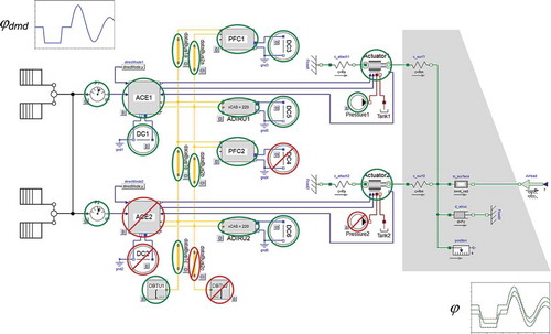
Figure 1 illustrates the concept of state space simulation by the example of an aircraft’s rudder control and actuation system. The image is actually the top level view of a corresponding Modelica model that is described in section 6.3 of [3]. Using a rudder position demand signal ${\phi }_{\mathrm{d}\mathrm{m}\mathrm{d}}$, the system model is simulated for combinations of intact and failed components. (The image shows just one of a multitude of combinations.) Whether the system operates or fails is identified by comparison of the simulated rudder position $\phi$ to the demand ${\phi }_{\mathrm{d}\mathrm{m}\mathrm{d}}$ (see Section 2.2). Section 3 explains in detail how method DMP uses graph algorithms to counter the problem of exponential growth of a system’s state space.

Figure 1. State space simulation of an aircraft’s rudder control and actuation system.

Other approaches to automated safety or reliability analysis based on multi-domain object-oriented modelling exist. One of them has been described by Bunus and Lunde [4] in 2008 that is dedicated particularly to model-based diagnosis, that is, detection and isolation of failures in a technical system. For these purposes, the approach uses algebraic equations and constraints (inequalities) but no differential equations. Hence, it enables simulation of steady-state but rules out simulation of transient effects. Another approach has been described by Papadopoulos et al. [5] in 2001 that conducts semi-automatic synthesis of fault-trees by evaluation of failure annotations included in the components of a system model.

The DMP method described in this article differs from the existing approaches, in so far that differential-algebraic equations (DAE) are used for modelling and simulation (not just annotating) of failures. This enables the conducting of all other studies that initially motivated the implementing of a model of a fault-tolerant system.

For instance, with regard to aircraft electric networks, simulation of normal, abnormal or degraded operation permits the conducting of an electric loads analysis that reveals the most demanding cases for the components (e.g. generators, contactors, wires) of the network. These cases dictate the dimensioning of components and, in turn, their weight. Hence, such an electric network model can be used also for consideration of the network components capabilities and a balancing of all power needs, thus minimizing the dimensioning of components and, eventually, overall system weight. Corresponding work is documented in [6] and [7].

In addition, the DMP method encourages that safety or reliability analyses be conducted frequently during the system development process, which keeps them up-to-date especially when a system’s design is changed. The aim is improvement of system development and safety assessment processes, according to the concept of model-based systems engineering (MBSE).

2. Modelling approach

This section refers to the approach selected for the modelling of fault-tolerant systems and the necessary additions.

2.1. Modelling of failures

Minimal path set detection by method DMP requires that failure of a system can be simulated in addition to its normal behaviour. Thus, the modelling has to be supplemented by equations that reflect failures of system components and, if applicable, by operating logics that determine how a system reacts to the occurrence of component failures.

Model parameter values are changed in order to represent a failure. In doing so, the model equations remain the same (structure-invariant approach). For example, an open circuit (O/C) failure of an electrical conductor is described by changing its resistance R from the nominal to a much larger value.

Figure 9 in Section 3.2.2 shows an electric heating circuit that is used for exemplification of the DMP method. Figure 2 shows a voltage source, voltage divider resistor and ground that are comprised in the circuit. A minimal path set analysis considers open circuit failures of these components that are modelled as follows.

Figure 2. An electric voltage source (a), a voltage divider resistor (b) and a ground (c).

Figure 3. Simulation of a flight control surface deflection angle $\phi$. System operates = sysOp for ${\phi }_1$. System failure = not sysOp for ${\phi }_2$, ${\phi }_3$.

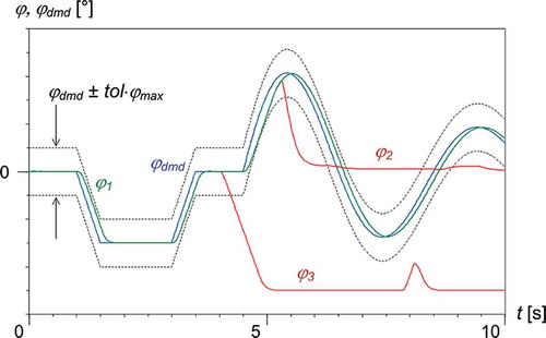
Figure 4. Exchange of power and signals across the edges in a coherent set of nodes.

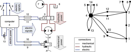
Figure 5. Coherent (a), (b), (c) and incoherent sets of nodes (d), (e) in a graph.

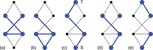
Figure 6. Components and connections in a multi-domain object-oriented model.

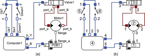
Figure 7. Adjacency list AL and graph for Figure 6(b) .

Figure 8. Flow chart of minimal path set detection algorithm DMP.

Figure 9. Redundant electric heating circuit.

The voltage source shown in Figure 2(a) is modelled as a series connection of an ideal voltage source $V_0$ with an internal resistance R. The voltage at the pins is $V=(V_0-R)i$, with $R=R_{\mathrm{n}\mathrm{o}\mathrm{m}}=1\mathrm{m}\mathrm{\Omega }$ if the source is intact and $R=R_{\mathrm{O}/\mathrm{C}}=1\mathrm{k}\mathrm{\Omega }$ (example values) if it has failed. The same concept of shifting the resistance R value to distinguish between the intact state and open circuit failure is used for the voltage divider resistor (Figure 2(b)) and ground element (c) models.

Large, realistic examples of aircraft on-board system models including further component failures, for example, mechanical disconnection or loss of hydraulic pressure, are provided in [3,8–10]. In conducting a state space simulation, method DMP activates component failures by directly accessing the relevant model parameters. Alternatively, a universal fault triggering network described by van der Linden [11] can be used for activation of failures.

Provided that the preconditions (see Section 3.1.2) are met, DMP can be used also if the structure of the model equations is changed to represent failures. Such a structure-variant, multi-mode approach is described by Elmqvist et al. [12].

A failure rate parameter ${\lambda }_i$ is stored in each component model that includes failure. Since the ${\lambda }_i$ values are used only for post-processing (see Equations (2) and (3)), they can be inserted also as custom annotations; a concept described by Zimmer et al. [13].

2.2. Indication of system status

Safety or reliability assessment requires the analyst to define criteria that decide if a system operates normally or if it fails. Such criteria have to be implemented in a system model, in order to compute a sysOp output signal that indicates the system status (operation or failure). In case of the flight control and actuation system shown in Figure 1, sysOp can be determined by comparing the actual (simulated) position $\phi$ of the controlled surface with the demand ${\phi }_{\mathrm{d}\mathrm{m}\mathrm{d}}$ (model input).

Suppose that the system model is simulated for the position demand ${\phi }_{\mathrm{d}\mathrm{m}\mathrm{d}}$ as shown in Figure 3. The capability of the system to move the surface accordingly depends on the status (intact or failed) of its components. A tolerance band is defined that is bounded by ${\phi }_{\mathrm{d}\mathrm{m}\mathrm{d}}$ $\pm$ tol ${\phi }_{\mathrm{m}\mathrm{a}\mathrm{x}}$, where tol is the tolerance, for example, 0.05, and ${\phi }_{\mathrm{m}\mathrm{a}\mathrm{x}}$ is the maximum surface deflection angle, for example, 25°. If the simulated deflection angle stays within the tolerance band, as is the case for ${\phi }_1$ in this example, then ‘system operates’ = sysOp is indicated. If the system cannot move the surface according to the demand, as occurs for ${\phi }_2$ and ${\phi }_3$, then ‘system failure’ = not sysOp is indicated.

The capability of the system to follow demands is examined by the minimal path set detection method DMP for multiple combinations of intact and failed components. In so doing, sysOp is evaluated for correlation with the respective component states.

3. A method for minimal path set detection

In this section, the DMP method is described that solves the problem of determining the failure probability of a system by detecting its minimal path set. DMP draws on a representation of the system model object structure as a graph and on simulation. Minimal path set analysis generally assumes that a system and its components are two-state, intact or failed, as explained in section 2.3 of [14].

The DMP method is a state space simulation. In this context, the state space denotes the set of all combinations of intact and failed components of a system. As is obvious, the size of the state space grows exponentially with the number of components of a system. In order to prevent unfeasibility of the DMP method due to this growth phenomenon also known as ‘combinatorial explosion’, algorithms founded on graph theory are devised for evaluation of the graph that corresponds to an object-oriented system model. Most combinations of intact and failed components, that is, a large part of a system’s state space, can be neglected as a result of evaluating the graph. Then, the system model is simulated only for the remaining part of the state space, which considerably reduces the computing effort.

3.1. Definitions and preparations

3.1.1. Definitions

Definitions are provided of the terms used in the following for the DMP method:

• Set. A defined collection of distinct objects, for example, the components of a system.

• Subset. A is a subset of B, $A\subseteq B$, if every object of A is also an object of B, for example, $\left\{1,2,3\right\}\subseteq \left\{1,2,3\right\}$. If A is a subset of but unequal to B, then A is a proper subset of B, $A\subset B$, for example, $\left\{1,2\right\}\subset \left\{1,2,3\right\}$.

• Superset. A is a superset of B, $A\supseteq B$, if every object of B is also an object of A, for example, $\left\{1,2,3\right\}\supseteq \left\{1,2,3\right\}$. If A is a superset of but unequal to B, then A is a proper superset of B, $A\supset B$, for example, $\left\{1,2,3\right\}\supset \left\{1,2\right\}$.

• Difference set. $A\mathrm{\setminus }B$ denotes the set of elements that are members of A but not of B, for example, $\left\{1,2,3\right\}\mathrm{\setminus }\left\{2\right\}=\left\{1,3\right\}$, or $\left\{1,2,3\right\}\mathrm{\setminus }\left\{4\right\}=\left\{1,2,3\right\}$.

• Component. A distinct element of a system. In this article, components are also called nodes.

• Combination. A set of intact components of a system.

• Path. A set of intact components that causes a system to operate.

• S–T path. A source-to-target path in a graph.

• Path set. A set of paths of a system.

• Minimal path. A path that cannot be reduced without causing system failure.

• Minimal path set. The set of all minimal paths of a system.

• Graph. A representation of a set of objects, for example, the components (nodes) of a system, and of the connections between them.

• Node. An object in a graph. Nodes are also called components in this article.

• Edge. A link that connects a pair of nodes in a graph.

• Articulation. A node in a graph (or path) that, if removed, causes disconnection of the graph (or path) into several subgraphs.

• Subgraph. A part of a graph whose set of nodes and set of edges are subsets of those of the graph, the set of edges being restricted to the subset of nodes.

• Density. The density d of a graph is generally, for example, in [15], defined by

  (1) $d\left(N,E\right)=2E/N\left(N-1\right),$(1)

where N and E denote the numbers of nodes and edges of the graph, respectively.

Probability computation. The probability of system operation or failure is computed from the system’s minimal path set in applying the reliabilities of its components. Let $C_i$ denote the intact state of component i. Then, the probability of occurrence P of a minimal path MP is, see [16],

(2) $\begin{array}{rl}& P\left(MP\right)=P\left(C_1\wedge C_2\wedge \dots \right)\mathrm{\forall }{C}_i\in MP\\ & P\left(MP\right)=\prod _{C_i\in MP}P\left(C_i\right)=\prod _{C_i\in MP}{R}_i\left(t\right),R_i\left(t\right)=e^{-{\lambda }_{i}t}\end{array},$(2)

with the component reliabilities $R_i$, failure rates ${\lambda }_i$ and exposure time t. Exponentially distributed lifetimes are assumed. Other lifetime models, for example, Weibull distribution, can be used as well. The probability of system operation $R_{\mathrm{s}\mathrm{y}\mathrm{s}}(t)$ is computed from the probabilities of the minimal paths by

(3) $\begin{array}{cc}{R}_{\mathrm{s}\mathrm{y}\mathrm{s}}(t)& =P\left(M{P}_1\vee \dots \vee M{P}_r\right)\\ & =\sum _{j=1}^{r}P\left(M{P}_j\right)-\sum _{j=1}^{r-1}\sum _{k=j+1}^{r}P\left(M{P}_j\wedge M{P}_k\right)+\dots \\ & +{\left(-1\right)}^{r+1}P\left(M{P}_1\wedge M{P}_2\wedge \dots \wedge M{P}_r\right),\end{array}$(3)

where r is the number of all minimal paths in the set. Equation (3) is called Poincaré formula. It is evaluated for illustration at the end of Section 3.2.2.

3.1.2. Properties of minimal paths and requirements for detection

This subsection explains the assumptions and requirements that apply to method DMP:

1. The system behaves monotonously. This refers to a system that operates if all its components are intact and fails if all components fail. If the system operates while not all components are intact, it continues operating if any further component becomes intact. Conversely, if the system has failed, it remains failed if any further component fails. This definition of monotony is common in safety analysis. For instance, it can be found in section 14.2 of [16].

2. Every real world component is represented by one model object and by one node in a corresponding graph. No component is represented by two or more model objects or nodes.

DMP relies on a representation of the object structure of a system model as a graph. Nodes of the graph represent components, and edges the connections between components. The establishing of a graph is described in Section 3.1.3. The properties of minimal paths, and in particular their situation in the graph, are explained in the following, which then proceeds to further requirements for method DMP.

Depending on the system model and, if applicable, the marking of sources (S) and targets (T) in the corresponding graph, some S–T paths are minimal paths. This is true, for instance, for the electric network models shown in [8,9], where also related detection methods are described. In general, however, what is known is only that a minimal path consists of one or more connected nodes.

This is explained by Figure 4 that depicts a part of a flight control surface actuation system model and its accompanying graph. The edges of the graph correspond to the interfaces that exchange power, material or signals among the components (nodes) of a system. This exchange among neighboured nodes enables a system to operate. No other nodes are situated between any of those nodes that exchange power, material or signals and hence belong to a minimal path. Thus, only a coherent set of nodes can be a minimal path. The following defines a coherent set of nodes:

Definition 1. A set of nodes in a graph is coherent if any two nodes of the set are connected through a series of edges and through only those nodes that belong to the set.

Figure 5 shows coherent and incoherent sets of nodes (marked blue) for illustration. An S–T path, such as (c), is hence a special case of a coherent set of nodes.

Coherence (interconnection) of intact nodes in the system graph is a precondition for a minimal path. Removing a node from a minimal path interrupts the exchange of power, material or signals among the nodes of the minimal path. If no other minimal paths exist, the system fails. If the system operates with an incoherent set of intact nodes, some nodes can be removed from the set, that is, fail, without interrupting the exchange of power etc. Such a set of nodes is therefore a path but not a minimal path. Thus, the third assumption for method DMP is:

• (3) Only a coherent set of intact nodes in a system graph can be a minimal path.

Because not every coherent set of intact nodes is a minimal path, the system model is simulated to determine which ones are actually minimal paths.

3.1.3. Graph representation of multi-domain object-oriented models

A graph is defined by its adjacency list (array AL). In AL, each row corresponds to a node of the graph. The neighbours of a node are stored in the respective row of AL, as will be illustrated. If more than one connection exists between two components of a model, this is reflected by a single edge in the graph. (That is, in each row of AL, any node is stored not more than once.) It is only relevant that any two nodes of the graph are connected, but it is not important whether the two nodes are connected by one or more than one edge. Additionally, the interface types are not evaluated by method DMP, so they are not reflected in the graph.

For illustration, the adjacency list is indicated for a part of the system model depicted in Figure 4. Figure 6(a) shows the component (node) and interface names, and the indices in (b). The numbering of nodes – encircled in (b) – corresponds to Figure 4. The connections via mechanical flanges, hydraulic ports, electric pins etc. are declared in the model by the connect () statements below. They are expressed in terms of the component and interface names (left column), and in terms of component and interface indices (right column).

1. connect(POB1.flange_a, Motor1.flange);(1.1, 2.3)

2. connect(Motor1.port_a, Valve1.port_A);(2.1, 3.1)

3. connect(Motor1.port_b, Valve1.port_B);(2.2, 3.2)

4. connect(POB1.p, Computer1.p_B);(1.2, 4.5)

5. connect(Valve1.p, Computer1.p_V);(3.3, 4.4)

6. connect(Computer1.Sw1, Up1.p);(4.2, 5.1)

7. connect(Up1.p, Down1.p);(5.1, 6.1)

8. connect(Computer1.Up1, Up1.n);(4.1, 5.2)

9. connect(Computer1.Down1, Down1.n);(4.3, 6.2)

The algorithm that actually prepares an adjacency list AL is described in detail in subsection 3.1.3 of [3]. First, it stores the list of connect () statements in a stack named S_conn (index format). Then, it starts an i-loop over all nodes. For each node, the algorithm parses the rows of S_conn, that is, the connect () statements, to check if this node (node i) occurs in it. If yes, the algorithm checks if AL already indicates that node i and the other node of the corresponding connect () statement are connected. If not, then these nodes are stored in the respective two rows of AL. The connect () statement is deleted from stack S_conn, since it does not need to be evaluated again in subsequent loop iterations.

A special case occurs if more than one node is directly or indirectly connected to one and the same interface of a node, as happens for the sixth and seventh connections of the example: Computer1.Sw1 (4.2) is connected to Up1.p (5.1), and in turn Up1.p (5.1) is connected to Down1.p (6.1). Actually, there is a direct connection between (4.2) and (6.1). It only appears to be indirect, across (5.1), because each connect () statement links exactly two nodes. To reflect that a direct connection exists between (4.2) and (6.1), the algorithm introduces an auxiliary node (14). Auxiliary nodes do not represent any real or model object; rather, they are introduced to ensure that coherent sets of nodes are correctly detected by method DMP. An auxiliary node is stored as an additional row in the adjacency list AL.

Figure 7 specifies the adjacency list for Figure 6(b) in terms of the node indices and shows the corresponding graph.

3.2. Detection of minimal paths

Method DMP is capable of detecting the minimal path set if conditions (1), (2) and (3) defined in Section 3.1.2 are fulfilled. The detection starts with all system components (nodes) intact. Nodes are then successively removed from the system graph, which corresponds to component failures. The model is simulated to identify if the system still operates or fails.

Articulations can occur in the graph that, if removed, cause disconnection of the graph into several subgraphs. Since only a coherent set of intact nodes can be a minimal path, splitting up the graph at articulations reduces the state space and thus the number of simulations. The lower the density of a system graph is, the more articulations occur within it and thus fewer simulations are required. For completeness, method DMP allows that articulations can also belong to a minimal path.

3.2.1. Detection algorithm

Figure 8 shows a flow chart of the detection algorithm. It consists of a preparation phase (steps DMP.1–4) and the actual, iterative detection process (steps DMP.5–17). Steps DMP.3, 8 and 11–16 refer to lower level algorithms that are described in detail, including code, in [3]. The meaning of the symbols used is as follows:

nr number of all components that can fail of a system

n_Loopiteration counter of detection process

rnnode(s) to be removed from a path of array PS_prev

PS, PS_prevarrays of path sets in the actual and previous iteration, respectively, of the detection process

isMinPS, isMinPS_prevBoolean arrays that store if a path in array PS or PS_prev is minimal

np, np_prevnumber of paths stored in PS and PS_prev, respectively

SFarray for storing combinations that cause system failure

nsfnumber of combinations stored in array SF

In the preparation phase, the necessary data are retrieved from the system model (step DMP.1). Then, the model is simulated to check if the system operates for the set of initially intact components (nodes). To this end, the model output sysOp is evaluated. A monotonous system will operate, and the procedure is continued only in this case (step DMP.2). If the system fails, no minimal path can be detected, and the process is aborted. Next, a graph (adjacency list) of the system model is established (step DMP.3, see Section 3.1.3). Then, several arrays are initialized (step DMP.4) for the detection process.

At the start of an iteration, the paths detected so far, their number, as well as the information whether they are minimal are assigned to PS_prev, np_prev and isMinPS_prev. Arrays PS, isMinPS and the counter np are reset (step DMP.5). Then, n_Loop is increased by one. Next, combinations are generated from the paths in PS_prev. If the ith path, denoted by PS_prev[i,:], is minimal (checked in step DMP.7), then it is not further reduced, because any subset of a minimal path causes system failure. If the ith path is not minimal, then all subsets are generated that remove one intact node rn from the path (step DMP.8): PS_prev[i,:]\{rn} for all rn $\in$ PS_prev[i,:] and rn $\in$ {1, nr}. If node rn is an articulation of path PS_prev[i,:], the corresponding subgraphs of PS_prev[i,:] are generated. Articulations and subgraphs are determined by an algorithm based on depth-first search described by Tarjan in [17]. Along with each subgraph, the non-articulations of PS_prev[i,:] that also belong to the respective subgraph are stored. This information is used later, in step DMP.13, to generate combinations that remove two or more non-articulations from a path, dependent on the simulation result (step DMP.11). Due to system monotony, any subset of a path is generated only if it is not a subset of any combination stored in SF that causes system failure. Thus, if no subset is generated from path PS_prev[i,:] in step DMP.8, then the system fails for every subset of this path; it is minimal and is marked by isMinPS_prev[i]: = true. The generation of subsets of paths ends after every path in PS_prev has been processed, that is, i > np_prev (step DMP.10).

Next (step DMP.11), the model is simulated for every generated combination in order to determine if the system is operating. From the simulation result (sysOp or not sysOp), it is first determined which paths in PS_prev are minimal. If a path is minimal, it is stored in PS and marked as minimal in isMinPS. Then, dependent on whether they cause system operation or failure, the combinations are stored either in PS or in SF, and the respective counter (np or nsf) is increased (step DMP.12).

For those paths in PS that were established due to an articulation and that are no superset of any other path, combinations are generated that remove two or more non-articulations from the original path in PS_prev (step DMP.13). This is necessary since articulations can also belong to a minimal path. The system model is then simulated for the generated combinations. Dependent on the simulation result, a combination is stored either in PS or SF (steps DMP.14 and 15).

Next, array PS is tidied up by deleting those paths that are a superset of any other path (step DMP.16). A path can be minimal only if it is not a superset of any other path. If every of the np paths in PS is marked as minimal (step DMP.17), the detection is complete and the process ends. Otherwise, the process continues with a new iteration at step DMP.5.

3.2.2. A minimal path set detection example

The detection algorithm DMP is illustrated by means of the redundant electric heating circuit shown in Figure 9. This small, academic example permits a complete illustration of the detection algorithm, addressing all its core characteristics. For an aircraft system model of the size and complexity shown in Figure 1, the corresponding graph is quite large and hence the course of the detection algorithm is far too extensive for illustration.

The electric circuit shown in Figure 9 consists of two heating elements 1, 4 that are resistive voltage dividers (refer also to Figure 2). Each heating element is connected to a voltage source 2, 6 and to a ground element 3, 5. The circuit works (sysOp) i.e. heat is produced, if current flows through at least one of the two heating elements. This occurs if all components of at least one of the two following sets of components are intact: $\left\{1,2,3\right\}$ or $\left\{4,5,6\right\}$. Obviously, each of these two sets is a minimal path according to the definition in Section 3.1.1. In addition, the heating elements 1, 4 are interconnected, and a supplemental ground 7 is connected to voltage source 6. This arrangement allows for another way of operating the circuit: Current can flow from voltage source 6 (grounded by means of 7) through the heating resistors 4 and 1 to ground 3; thus $\left\{1,3,4,6,7\right\}$ is another minimal path of the circuit.

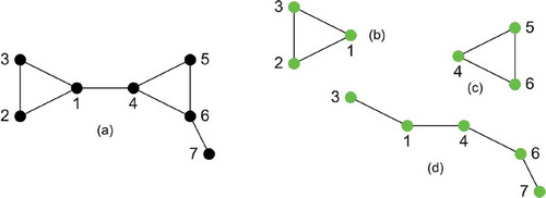
The graph corresponding to this circuit is shown in Figure 10(a). Its minimal path set (consisting of three minimal paths) PS $=\left\{\left\{1,2,3\right\},\left\{4,5,6\right\},\left\{1,3,4,6,7\right\}\right\}$ is indicated by the nodes marked green in Figure 10(b–d).

Figure 10. Graph (a) of electric heating circuit shown in Figure 9 and its three minimal paths (b), (c), (d) .

The detection algorithm DMP proceeds as follows. In the tables below, column ’row’ indicates the progress of the algorithm in terms of ‘n_Loop-number of comb’, for example, '0–1ʹ denotes combination 1 of iteration 0 (n_Loop = 0). Entries 'x’ and '–’ in the tables connote 'yes’ and 'no’ (or ’not applicable’), respectively.

The meaning of the symbols used is as follows, as yet not defined:

isArtindicates if rn is an articulation of the respective path

combgenerated combination of intact nodes

simCarray of generated combinations, input for simulations of the system model

sysOparray of simulation result (system operates or not) for every combination in simC

nonArt non-articulation nodes of a path in PS_prev that also belong to a generated subgraph

In the preparation phase it is checked if the system operates when all its components are intact (step DMP.2 in Figure 8). Thus, the simulation input simC is as indicated in Table 1. At this initial stage, no path has yet been detected and PS_prev is empty.

Table 1. Combinations tested (by simulation of system model) at initial stage of detection process.

					comb stored in simC
Row	PSprev	rn	isArt	comb	No	Yes	sysOp	nonArt
0–1	–	–	–	{1, 2, 3, 4, 5, 6, 7}	–	x	x	–

The system operates, so the set of initially intact nodes is stored as a single, non-minimal path (np = 1) in PS (step DMP.4). SF is empty (nsf = 0), as Table 2 indicates.

The process continues with iteration one (n_Loop = 1). The path data are assigned to PS_prev, isMinPS_prev and np_prev. PS, isMinPS and np are reset (step DMP.5). Combinations are then generated from path PS_prev[1,:] as follows (step DMP.8): Node 1 is an articulation. The path splits into two subgraphs $\left\{2,3\right\}$ and $\left\{4,5,6,7\right\}$ due to the removal of node 1. The non-articulations of the original path PS_prev[1,:] that also belong to the respective subgraphs are $\left\{2,3\right\}$ and $\left\{5,7\right\}$. Node 2 is not an articulation, thus a combination is generated by removing node 2 from PS_prev[1,:], and likewise for nodes 3, 5 and 7. Altogether, 10 combinations are generated for simulation of the system model. They are listed in Table 3 and are shown in Figure 11 using the same row indices 1–1, 1–2, etc.

Table 2. Path set after initial stage of detection process.

PS	isMinPS	SF
{1, 2, 3, 4, 5, 6, 7}	–	–

Table 3. Combinations tested during first iteration of detection process.

					comb stored in simC
Row	PSprev	rn	isArt	comb	No	Yes	sysOp	nonArt
1–1	{1, 2, 3, 4, 5, 6, 7}	{1}	x	{2, 3}	–	x	–	{2, 3}
1–2		{1}	x	{4, 5, 6, 7}	–	x	x	{5, 7}
1–3		{2}	–	{1, 3, 4, 5, 6, 7}	–	x	x	-
1–4		{3}	–	{1, 2, 4, 5, 6, 7}	–	x	x	-
1–5		{4}	x	{1, 2, 3}	–	x	x	{2, 3}
1–6		{4}	x	{5, 6, 7}	–	x	–	{5, 7}
1–7		{5}	–	{1, 2, 3, 4, 6, 7}	–	x	x	-
1–8		{6}	x	{1, 2, 3, 4, 5}	–	x	x	{2, 3, 5}
1–9		{6}	x	{7}	–	x	–	{7}
1–10		{7}	–	{1, 2, 3, 4, 5, 6}	–	x	x	-

Figure 11. Combinations tested during first iteration of detection process.

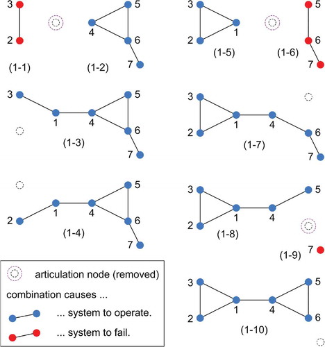
The simulation result of step DMP.11 is listed in column sysOp of the table and also visualized in Figure 11: Combinations of intact nodes that cause the system to operate are marked blue, those causing system failure are marked red. The simulation result indicates that path PS_prev[1,:] is not minimal, because the system operates for subsets of it, namely for those in rows 1–2, 1–3, 1–4, 1–5, 1–7, 1–8 and 1–10. These combinations are stored as paths in PS, np = 7. The other combinations in rows 1–1 and 1–6 are stored in SF, nsf = 2 (step DMP.12). The one in row 1–9, $\left\{7\right\}$, is not stored in SF as it is a subset of $\left\{5,6,7\right\}$.

At this stage, two of the seven paths in PS are not supersets of any other path, namely rows 1–2 and 1–5 in Table 3 (marked bold). Other paths can exist that include some of the articulations of the original path PS_prev[1,:]. To assure that such paths are detected, further combinations that are no superset of any path in PS – in this case $\left\{4,5,6,7\right\}$ and $\left\{1,2,3\right\}$ – must be generated (step DMP.13). Such combinations remove as many non-articulations from the original path as non-superset paths were deduced from it, namely two (rows 1–2 and 1–5) in the case of PS_prev[1,:]. To avoid generating supersets, one node of every set of non-articulations, $\left\{5,7\right\}$ and $\left\{2,3\right\}$, is removed from the original path, respectively. Thus, the combinations PS_prev[1,:] $\mathrm{\setminus }\left\{2,5\right\}$, PS_prev[1,:] $\mathrm{\setminus }\left\{2,7\right\}$, PS_prev[1,:] $\mathrm{\setminus }\left\{3,5\right\}$ and PS_prev[1,:] $\mathrm{\setminus }\left\{3,7\right\}$ are generated. These are listed in rows 1–11 through 1–14 of Table 4 and are shown in Figure 12. The paths denoted by rows 1–2 and 1–5 of Table 3 are shown again in the lower left part of the figure; due to this, it can be seen that neither generated combination, 1–11 through 1–14, is a superset of any of these paths.

Table 4. Combinations tested during first iteration that remove two non-articulations from PS_prev[1,:].

				comb stored in simC
Row	PSprev	rn	comb	No	Yes	sysOp
1–11		{2, 5}	{1, 3, 4, 6, 7}	–	x	x
1–12	{1, 2, 3, 4, 5, 6, 7}	{2, 7}	{1, 3, 4, 5, 6}	–	x	x
1–13		{3, 5}	{1, 2, 4, 6, 7}	–	x	–
1–14		{3, 7}	{1, 2, 4, 5, 6}	–	x	x

Figure 12. Combinations tested during first iteration that remove two non-articulations from PS_prev[1,:].

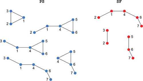
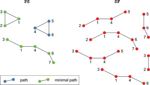
As before, the result of the simulation (step DMP.14) is indicated in column sysOp of Table 4 and shown in Figure 12. Consequently, three more paths are stored in PS, np $=7+3=10$, and one more combination in SF, nsf $=2+1=3$ (step DMP.15). The total number of simulations so far is n_sim $=1+10+4=15$. Supersets of paths are removed from PS, which leads to np $=5$ paths remaining after completion of step DMP.16. Table 5 and Figure 13 summarize the content of arrays PS and SF at this stage – end of the first iteration – of the detection process.

Table 5. Path set PS and combinations that cause system failure SF, as existent after first iteration of detection process.

PS	isMinPS	SF
{1, 2, 3}	–	{1, 2, 4, 6, 7}
{1, 2, 4, 5, 6}	–	{2, 3}
{1, 3, 4, 5, 6}	–	{5, 6, 7}
{1, 3, 4, 6, 7}	–
{4, 5, 6, 7}	–

Figure 13. Path set PS and combinations that cause system failure SF, as existent after first iteration of detection process.

Since none of the paths in PS is marked as minimal (step DMP.17), the process continues with a second iteration (n_Loop = 2). The path data are assigned to PS_prev, isMinPS_prev and np_prev. PS, isMinPS and np are reset (step DMP.5). Then, combinations are generated (step DMP.8) from each of the np_prev = 5 paths in PS_prev as listed in Table 6. Three combinations are generated from PS_prev[1,:] $=\left\{1,2,3\right\}$, but only one is stored in simC for simulation. The other two are not stored in simC because they are a subset of a combination in SF, as indicated in rows 2–1 and 2–3. If a combination causes system failure, every subset of it causes system failure as well due to system monotony.

Table 6. Combinations tested during second iteration of detection process.

					comb stored in simC
Row	PSprev	rn	isArt	comb	No	Yes	sysOp	nonArt
2–1		{1}	–	{2, 3}	$\subseteq \left\{2,3\right\}$	–	–	–
2–2	{1, 2, 3}	{2}	–	{1, 3}	–	x	–	–
2–3		{3}	–	{1, 2}	$\subseteq \left\{1,2,4,6,7\right\}$	–	–	–
2–4		{1}	x	{2}	$\subseteq \left\{1,2,4,6,7\right\}$	–	–	–
2–5		{1}	x	{4, 5, 6}	–	x	x	{5,6}
2–6		{2}	–	{1, 4, 5, 6}	–	x	x	–
2–7	{1, 2, 4, 5, 6}	{4}	x	{1, 2}	$\subseteq \left\{1,2,4,6,7\right\}$	–	–	–
2–8		{4}	x	{5, 6}	$\subseteq \left\{5,6,7\right\}$	–	–	–
2–9		{5}	–	{1, 2, 4, 6}	$\subseteq \left\{1,2,4,6,7\right\}$	–	–	–
2–10		{6}	–	{1, 2, 4, 5}	–	x	–	–
2–11		{1}	x	{3}	$\subseteq \left\{2,3\right\}$	–	–	–
2–12		{1}	x	{4, 5, 6}	Exists in simC	–	x	–
2–13		{3}	–	{1, 4, 5, 6}	Exists in simC	–	x	–
2–14	{1, 3, 4, 5, 6}	{4}	x	{1, 3}	exists in simC	–	–	–
2–15		{4}	x	{5, 6}	$\subseteq \left\{5,6,7\right\}$	–	–	–
2–16		{5}	–	{1, 3, 4, 6}	–	x	–	–
2–17		{6}	–	{1, 3, 4, 5}	–	x	–	–
2–18		{1}	x	{3}	$\subseteq \left\{2,3\right\}$	–	–	–
2–19		{1}	x	{4, 6, 7}	$\subseteq \left\{1,2,4,6,7\right\}$	–	–	–
2–20		{3}	–	{1, 4, 6, 7}	$\subseteq \left\{1,2,4,6,7\right\}$	–	–	–
2–21	{1, 3, 4, 6, 7}	{4}	x	{1, 3}	Exists in simC	–	–	–
2–22		{4}	x	{6, 7}	$\subseteq \left\{5,6,7\right\}$	–	–	–
2–23		{6}	x	{1, 3, 4}	–	x	–	{3}
2–24		{6}	x	{7}	$\subseteq \left\{5,6,7\right\}$	–	–	–
2–25		{7}	–	{1, 3, 4, 6}	Exists in simC	–	–	–
2–26		{4}	–	{5, 6, 7}	$\subseteq \left\{5,6,7\right\}$	–	–	–
2–27		{5}	–	{4, 6, 7}	$\subseteq \left\{1,2,4,6,7\right\}$	–	–	–
2–28	{4, 5, 6, 7}	{6}	x	{4, 5}	–	x	–	{4,5}
2–29		{6}	x	{7}	$\subseteq \left\{5,6,7\right\}$	–	–	–
2–30		{7}	–	{4, 5, 6}	Exists in simC	–	x	–

Any combination is stored only once in simC, as indicated in row 2–12, for instance. Eight combinations are stored altogether for simulation in step DMP.11.

The simulation result (column sysOp) indicates that PS_prev[1,:] $=\left\{1,2,3\right\}$ and PS_prev[4,:] $=\left\{1,3,4,6,7\right\}$ are minimal, because the system fails for every respective subset. These paths are stored in PS and marked as minimal in isMinPS (step DMP.12). In addition, two non-minimal paths, $\left\{4,5,6\right\}$ in row 2–5 and $\left\{1,4,5,6\right\}$ in row 2–6, are stored in PS; the latter will be removed in step DMP.16.

It is not necessary in this iteration to generate combinations that remove two or more non-articulations from any path in PS_prev. The reason is: At most one subgraph that causes system operation is deduced from any path in PS_prev. In the case of PS_prev[2,:] $=\left\{1,2,4,5,6\right\}$, subgraphs $\left\{2\right\}$, $\left\{4,5,6\right\}$ and $\left\{1,2\right\}$, $\left\{5,6\right\}$ are generated due to articulations 1 and 4, respectively. The system operates only for $\left\{4,5,6\right\}$. In order to generate every combination from PS_prev[2,:] that is no superset of $\left\{4,5,6\right\}$, it is sufficient to remove one non-articulation from PS_prev[2,:]. These combinations are generated already in step DMP.8, as Table 6 shows (rows 2–9 and 2–10).

Thus, np = 4 paths are stored in PS of which two are marked as minimal. nsf $=3+3=6$ combinations are stored in SF. The total number of simulations so far is n_sim $=15+8=23$. np = 3 paths remain in PS after removal of supersets in step DMP.16. The content of arrays PS and SF at this stage – end of the second iteration – of the process is summarized in Table 7 and Figure 14.

Table 7. Path set PS and combinations that cause system failure SF, as existent after second iteration of detection process.

PS	isMinPS	SF
{1, 2, 3}	x	{1, 2, 4, 5}
{1, 3, 4, 6, 7}	x	{1, 2, 4, 6, 7}
{4, 5, 6}	–	{1, 3, 4, 5}
		{1, 3, 4, 6}
		{2, 3}
		{5, 6, 7}

Figure 14. Path set PS and combinations that cause system failure SF, as existent after second iteration of detection process.

Since not all paths are marked as minimal, the process enters a third iteration, n_Loop = 3. Again, the path data are assigned to PS_prev, isMinPS_prev and np_prev. PS, isMinPS and np are reset. Then, combinations are generated only for the non-minimal path PS_prev[3,:] $=\left\{4,5,6\right\}$ in step DMP.8. As Table 8 shows, every generated combination is a subset of any combination in SF. This means that PS_prev[3,:] is also minimal, and no further simulations are necessary. Thus, the process is complete. The minimal path set of the example system (Figure 10) is correctly detected, as Table 9 indicates.

Table 8. Third iteration of detection process (no combinations tested).​​

					comb stored in simC
Row	PSprev	rn	isArt	comb	No	Yes	sysOp	nonArt
3–1		{4}	–	{5, 6}	$\subseteq \left\{5,6,7\right\}$	–	–	–
3–2	{4, 5, 6}	{5}	–	{4, 6}	$\subseteq \left\{1,3,4,6\right\}$	–	–	–
3–3		{6}	–	{4, 5}	$\subseteq \left\{1,2,4,5\right\}$	–	–	–

Table 9. Minimal path set detected after third iteration of the process.

PS	isMinPS
{1, 2, 3}	x
{1, 3, 4, 6, 7}	x
{4, 5, 6}	x

Next, the probability of system operation (or failure) is computed. For illustration, Equation (3) is evaluated for the detected minimal path set. With the component reliabilities $R_i=R_i(t)$, the probabilities of the minimal paths are

$P\left(P{S}_1\right)=R_1{R}_2{R}_3,P\left(P{S}_2\right)=R_1{R}_3{R}_4{R}_6{R}_7,P\left(P{S}_3\right)=R_4{R}_5{R}_6.$

For the second-order intersections, the probabilities are

$\begin{array}{cc}P\left(P{S}_1\wedge P{S}_2\right)& =R_1{R}_2{R}_3{R}_4{R}_6{R}_7,P\left(P{S}_1\wedge P{S}_3\right)=R_1{R}_2{R}_3{R}_4{R}_5{R}_6,\\ P\left(P{S}_2\wedge P{S}_3\right)& =R_1{R}_3{R}_4{R}_5{R}_6{R}_7.\end{array}$

The probability of the single third-order intersection is

$P\left(P{S}_1\wedge P{S}_2\wedge P{S}_3\right)=R_1{R}_2{R}_3{R}_4{R}_5{R}_6{R}_7.$

Employing these products, Equation (3) reads

$\begin{array}{cc}{R}_{sys}(t)& =R_1{R}_2{R}_3+R_1{R}_3{R}_4{R}_6{R}_7+R_4{R}_5{R}_6\\ & -\left(R_1{R}_2{R}_3{R}_4{R}_6{R}_7+R_1{R}_2{R}_3{R}_4{R}_5{R}_6+R_1{R}_3{R}_4{R}_5{R}_6{R}_7\right)\\ & +R_1{R}_2{R}_3{R}_4{R}_5{R}_6{R}_7.\end{array}$

If it is assumed that ${\lambda }_i={10}^{-}{ }^2/$h and $t=1$h, thus $R=R_i=0.990$, then the probability of system operation is $R_{sys}(1$h$)=2R^3+R^5-3R^6+R^7=0.99922$ or likewise, the probability of system failure is $F_{\mathrm{s}\mathrm{y}\mathrm{s}}(1$h$)=1-R_{\mathrm{s}\mathrm{y}\mathrm{s}}(1$h$)=7.8\cdot {10}^{-4}$.

3.2.3. Proof and boundary effort of detection method

The minimal path set detection method DMP gives a complete result when applied to any multi-domain object-oriented system model that fulfils the conditions (1), (2) and (3) stated in Section 3.1.2. In addition, the method is finite which means that it terminates when applied to any such model. The completeness and finiteness are proven in the following. The upper and lower bounds of the required computing effort are also derived.

Completeness. Consider a detection method that merely exploits the monotony of the analysed system. It starts with a set of all nodes as the initial path. Every combination is generated that removes a single node from the path. It is tested for each (by simulation of the model) if the system operates. Those combinations that cause system operation constitute a set of paths. In the set of paths, only those are kept that are no superset of any other, because only a non-superset path can be minimal. Thus, a complete path set of the system exists at the end of an iteration of the detection method.

A next iteration is entered. All combinations are generated that remove a single node from every path in the set of the previous iteration. In so doing, subsets of combinations that cause system failure are omitted. Due to monotony, if a combination causes system failure, the system remains failed if any node is removed from that combination. Again, testing the generated combinations leads to a complete set of paths, a next iteration is entered with all non-superset paths of the set, and so on. At some point it is found that the system fails on removal of any node from a path. Such a path is minimal by definition. The method continues reducing the other paths until all in the set of paths are minimal. Since every path was reduced by a single node from one iteration to the next, it is obvious that the method gives the complete minimal path set.

In addition to exploiting system monotony, method DMP benefits from the fact that only a coherent set of intact nodes can be a minimal path. Evaluation of the system graph hence reduces the number of simulations required for minimal path set detection.

A path is split into subgraphs at the articulations of the path. In this way, subgraphs are generated for every path that exists in the path set of the previous iteration of DMP. If two or more subgraphs of a path cause system operation, all combinations are generated that remove as many non-articulations from that path, as subgraphs were deduced from it that cause system operation. (Two or more nodes are removed, because all combinations that reduce a path by one of its non-articulations have been generated and tested in a preceding step.) In so doing, for the generated combinations to be no superset of any of the subgraphs of that path, each non-articulation removed from the path belongs to exactly one of its subgraphs. Thus, if any such combination causes system operation, it exists in the path set at the end of an iteration of DMP. It follows that the path set at the end of any iteration is complete, and hence method DMP is complete.

Finiteness. DMP commences with a set of all nodes of a monotonous system as the initial path. It tests if the system still operates for subsets of a (the initial or other) path. Every subset removes one or more nodes from a path. Nodes are never added to a path from one iteration to the next. DMP repeats gradually removing nodes until the system fails for all subsets of a path, that is, if that path is minimal. For those paths not yet identified as minimal, subsets of them are generated until they be reduced no further without causing system failure, that is, until every path is minimal. Then, the process ends. If every single node of a system constitutes a minimal path, the process ends after all nodes are failed. Due to monotony, a system fails if all its nodes fail. Thus, method DMP clearly terminates.

Effort. For illustration of the highest computing effort, consider a complete system graph that includes no articulations. Removal of any node gives a subsequent smaller complete graph. In addition, consider that every single node of the nr nodes of the system graph constitutes a minimal path. Then, the number of simulations in each iteration $n_{\mathrm{L}\mathrm{o}\mathrm{o}\mathrm{p}}$ of DMP is the binomial $C(nr,n_{\mathrm{L}\mathrm{o}\mathrm{o}\mathrm{p}})$. DMP iterates until all nodes are failed, that is, $n_{\mathrm{L}\mathrm{o}\mathrm{o}\mathrm{p}}=nr$. The total number of simulations is thus ${\sum }_{n_{\mathrm{L}\mathrm{o}\mathrm{o}\mathrm{p}}=0}^{nr}C(nr,n_{\mathrm{L}\mathrm{o}\mathrm{o}\mathrm{p}})=2^{nr}$, the same as a ‘brute force’ approach needs.

The lowest effort occurs if a system operates only with all its nodes intact (single minimal path that comprises all nodes of the system). Irrespective of the density of the system graph, DMP runs until iteration $n_{\mathrm{L}\mathrm{o}\mathrm{o}\mathrm{p}}=1$ is completed. The total number of simulations is hence ${\sum }_{n_{\mathrm{L}\mathrm{o}\mathrm{o}\mathrm{p}}=0}^{1}C(nr,n_{\mathrm{L}\mathrm{o}\mathrm{o}\mathrm{p}})=1+nr$.

The number of simulations required by DMP is thus bound by the upper limit $2^{nr}$ and lower limit $1+nr$. Between these bounds, the actual effort depends on the density of the system graph, the number of minimal paths and number of nodes thereof. The more effort is saved, the lower the density of a system graph is.

For illustration, Table 10 lists the number of simulations $n_{\mathrm{s}\mathrm{i}\mathrm{m}}$ for three detection cases. The number of edges and density (Equation (1)) of the respective graphs are denoted by E and d. The number of nodes is $N=nr=7$ for all cases. $n_{\mathrm{s}\mathrm{i}\mathrm{m}}$ is stated for method DMP, as well as a method that exploits the system ‘monotony only’ (no evaluation of the graph), as described. Case 2 corresponds to the example in Section 3.2.2. Case 1 relates to the same graph, but the system has one less minimal path. Case 3 assumes the same minimal path set as case 2, but the graph has a higher density (see Figure 15). The comparison shows that the fewer minimal paths exist and the lower the density of the graph, the smaller effort required by DMP. With an increasing number of minimal paths and graph density, the effort of DMP approaches that of the ‘monotony only’ method. A ‘brute force’ method neither evaluates the monotony of a system nor its graph; it thus requires $2^{nr}=128$ simulations for each case.

Table 10. Comparison of effort of minimal path set detection for three cases.

					$n_{\mathrm{s}\mathrm{i}\mathrm{m}}$
Case	System graph	E	d	PS	Monotony only	DMP
1	Figure 10(a)	8	0.381	{1, 2, 3}, {4, 5, 6, 7}	35	15
	Figure 10(a)	8	0.381	{1, 2, 3}, {4, 5, 6}, {1, 3, 4, 6, 7}	40	23
	Figure 15	10	0.476	{1, 2, 3}, {4, 5, 6}, {1, 3, 4, 6, 7}	40	34

Figure 15. An example system graph, higher density than that of Figure 10(a).

4. Conclusions

This article contributes a method called DMP for detection of the minimal path set of any fault-tolerant system that is represented as a multi-domain object-oriented model. It includes a description, exemplification and substantiation of the method.

DMP belongs to the class of state space simulations. Evaluation of the system graph reduces the number of simulations required, thus ensuring feasibility of DMP. It has been successfully tested on large, realistic models of safety relevant aircraft systems, such as the rudder control and actuation shown in Figure 1. For this matter, more detail can be obtained from section 6 of [3].

DMP can be employed throughout the system development process to keep the safety analysis up-to-date with design iterations. This is meaningful particularly if multi-domain object-oriented modelling is used already in systems engineering. DMP enhances the scope of application of a model while permitting all other simulation studies that originally motivated implementation of the model to be conducted. Thus, DMP supports the concept of model-based systems engineering (MBSE).

It must be borne in mind that all model-based safety analysis methods capture only those phenomena that are covered in the modelling. A model is always an abstraction of a real system and might hence be incomplete. Then again, using DMP ensures that all relevant failure conditions, at least in so far as modelled, are captured.

Acknowledgements

This research has received funding from the European Union’s 7th Framework Programme (FP7/2007-2013) for the CleanSky Joint Technology Initiative under grant agreement CSJU-GAN-SGO-2008-001. In addition, the author wishes to thank Dirk Zimmer for his help.

Disclosure statement

No potential conflict of interest was reported by the author.​​

Additional information

Funding

This research has received funding from the European Union’s 7th Framework Programme (FP7/2007-2013) for the CleanSky Joint Technology Initiative under grant agreement CSJU-GAN-SGO-2008-001.​​

References

- The Modelica Association, Modelica - A Unified Object-Oriented Language for Physical Systems Modeling - Tutorial, Version 1.4, December 2000. Available at https://www.modelica.org/documents/ModelicaTutorial14.pdf.
- The Modelica Association, Modelica standard library. Available at https://www.modelica.org/libraries.
- C. Schallert, Integrated Safety and Reliability Analysis Methods for Aircraft System Development using Multi-Domain Object-Oriented Models, Verlag Dr. Hut, München, Germany, 2015. ISBN: 978-3-8439-2408-5
- P. Bunus and K. Lunde, Supporting model-based diagnostics with equation-based object-oriented languages, Proceedings of the 2nd International Workshop on Equation-Based Object-Oriented Languages and Tools (EOOLT), Paphos, Cyprus, 2008, pp. 121–130.
- Y. Papadopoulos, J. McDermid, R. Sasse, and G. Heiner, Analysis and synthesis of the behaviour of complex programmable electronic systems in conditions of failure, Reliability Eng. Syst. Saf. 71 (2001), pp. 229–247. doi:10.1016/S0951-8320(00)00076-4
- C. Schallert, An integrated tool for aircraft electric power systems pre-design, Proceedings of the 2nd International Workshop on Aircraft System Technologies (AST), Hamburg, Germany, March 2009, pp. 39–48.
- D. Schlabe and D. Zimmer, Model-based energy management functions for aircraft electrical systems, SAE 2012 Power Systems Conference, paper no. 2012-01-2175, Phoenix, Arizona, October 2012.
- C. Schallert, Incorporation of reliability analysis methods with modelica, Proceedings of the 6th International Modelica Conference, Bielefeld, Germany, pp. 103–112, 2008.
- C. Schallert, Inclusion of reliability and safety analysis methods in modelica, Proceedings of the 8th International Modelica Conference, Dresden, Germany, 2011, pp. 616–627. doi: 10.3384/ECP11063616
- C. Schallert, A safety analysis via minimal path sets detection for object-oriented models, in Safety and Reliability: Methodology and Applications, T. Nowakowski, M. Mlynczak, A. Jodejko-Pietruczuk, S. Werbinska-Wojciechowska, eds., Taylor & Francis Group, London, UK, 2014. ISBN: 978-1-315-73697-6
- F. Van Der Linden, General fault triggering architecture to trigger model faults in Modelica using a standardized blockset, Proceedings of the 10th International Modelica Conference, Lund, Sweden, 2014, pp. 427–436. doi: 10.3384/ECP14096427
- H. Elmqvist, S.E. Mattsson, and M. Otter, Modelica extensions for multi-mode DAE-Systems, Proceedings of the 10th International Modelica Conference, Lund, Sweden, 2014, pp. 183–193. doi: 10.3384/ECP14096183
- D. Zimmer, M. Otter, H. Elmqvist, and G. Kurzbach, Custom annotations: Handling meta-information in modelica, Proceedings of the 10th International Modelica Conference, Lund, Sweden, 2014, pp. 173–182. doi: 10.3384/ECP14096173
- A. Birolini, Reliability Engineering †Theory and Practice (Fifth Edition), Springer-Verlag, Berlin, 2007. ISBN: 978-3-540-49388-4
- R. Diestel, Graph Theory (Graduate Texts in Mathematics), Springer-Verlag, Berlin, 2010. ISBN: 978-3-642-14278-9
- A. Meyna and B. Pauli, Taschenbuch der Zuverlässigkeits- und Sicherheitstechnik, Carl Hanser Verlag, München Wien, 2003. In German. ISBN: 3-446-21594-8
- R. Tarjan, Depth-First Search and Linear Graph Algorithms, SIAM J. Comput. 1 (2) (1972), pp. 146–160. doi:10.1137/0201010