Using spatial games to model dynamic evolutionary systems

ABSTRACT

Modelling the dynamics of evolutionary competing species on a physical grid is a challenging modelling problem. This paper presents a novel modelling approach for synthesizing evolutionary dynamics of competing species using a spatial game perspective. This modelling approach describes the movement of players (‘species’ in our context) across a lattice. The model is based on a payoff function which controls the move likelihood and direction of the players (‘predators’ and ‘preys’). Using simulated results, the paper provides a comparison between the spatial game model and an existing predator-prey dynamic model. Finally, a case study is performed to illustrate the application of this formalism and validate the model.

KEYWORDS:

• Spatial game
• dynamic evolutionary systems
• modelling
• predator and prey

1. Introduction

Spatial games are a combination of traditional game models and cellular automata, representing strategies, players, payoff function, structure of population, and updating rules. This methodology has been adopted to analyse various structures of populations [1–3]. This paper introduces for the first time spatial games as a modelling approach towards a system of evolutionary dynamics representing predator and prey.

The dynamic relationship between prey and its predator has long been one of the popular topics in both biology and mathematical biology because of its importance and universal existence. A large body of research has been devoted to modelling the biological mechanisms of dispersal, and the underlying prey and predator interaction.

Traditional modelling approaches use mathematical formulations mostly using differential equations and include various diffusion models. Introducing diffusion into a prey-predator system usually results in both species eventually reaching homogeneous distributions in the domain. Thus, in a reaction-diffusion system, diffusion models act as a stabilizer [4]. Under certain circumstances, diffusion can disrupt the process, causing non-uniform distribution in a prey-predator system. This destabilization is identified as diffusion-driven instability [5]. Traditional models have also considered influences such as odour [6–12] and mobility effect [13].

Compared to a traditional dynamic model, a spatial game model is more expressive and informative. It can capture the different habits and characteristics of the competing species and can be extended to other systems. It can also capture different mobility preferences of the species. For instance, the game-based perspective can be used to model the self-diffusion, cross-diffusion, chemo-taxis effect or even longer distance movement, previously discussed [14].

In this paper, the new approach is introduced and validated by comparing it with the more traditional cross-diffusion dynamic model and also validated with an actual field experiment.

The paper is organized as follows: Section 2 presents the new approach game-based model with payoff functions, probability move functions and interaction functions. Section 3 recalls the cross-diffusion model and Section 4 demonstrates the numerical simulation of both modelling approaches. Section 5 presents a comparison between the two modelling approaches and an actual field experiment. Section 6 discusses the results considering validation of the models and presents future work.

2. Game-based model

In this section, the modelling approach of the spatial game is introduced. Unique to this game-based approach is the ability to model the inclination of the ‘players’ to move to adjacent cells based on an incentive function. Thus, this model includes payoff functions, probabilistic functions and interaction functions all acting on a square grid. The payoff functions describe quantitatively the benefits that each species in each cell location (i, j) gains from moving into any of its neighbouring cells.

The probability functions calculate the likelihood of each member of cell location (i, j) to migrate to the neighbouring cells (based on the payoff functions), and the interaction functions describe the dynamic between prey and predator that coexist in each cell.

2.1. Payoff function

Using the spatial game approach it is assumed that prey and predator move in a reactionary way, meaning that the prey may be able to recognize the predator, and respond by moving away to avoid being caught. On the other hand, if predators recognize the prey, this may affect the rate and directions of their movement which may help them find prey. The payoff function of prey and predator at cell (i, j) is shown in Equation (1).

(1) $\begin{array}{c}Pu(i,j)=(\frac{k_1}{u+c_1}+e_1)(\frac{k_2}{v+c_2}+f)\\ Pv(i,j)=(k_3(u+c_3)+g)(\frac{k_4}{v+c_4}+h)\\ \hspace{0.17em}\end{array}$(1)

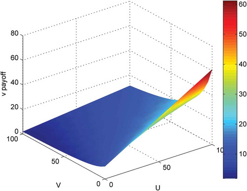
Where Pu denotes the payoff of prey, Pv indicates the payoff of predator. Parameters c₁, c₂, c₃, k₁, k₂, k₃, k₄, e₁, f, g, and h scale the payoff affections. As can be seen the prey’s function is inversely proportional to the number of prey (u) and predator (v) in cell (i, j). The predator’s payoff, on the other hand, is in proportion to the number of prey and inversely proportional to the number of other predators in cell (i, j). This implies that the prey prefers to move away from its own species (reduce competition for food) and understandably also from predators. The predators are attracted to the prey but prefer to move away from other predators. This function is not unique as there can be other functions that express the same type of preferences; however it seems to model the desired behaviour and is quite flexible using the tunable constants.

The behaviour of the payoff functions is demonstrated in Figure 1 and Figure 2, using a small example corresponding to different numbers of prey and predators in cell (i, j). The parameters used here are: k₁ = 250; k₂ = 100; k₃ = 1; k₄ = 10; e₁ = 0.01; f = 0.01; g = 0.01; h = 0.01; c₁ = 20; c₂ = 20; c₃ = 20; c₄ = 20; u = 0:5:100; v = 0:5:100; Figure 1 denotes that prey will get higher payoff if there were less prey and less predator within its cell. Figure 2 indicates that predator will have higher payoff with more prey and less predator.

Figure 1. Behaviour of payoff function of prey.

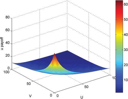
Figure 2. Behaviour of payoff function of predator.

2.2. Movement probability function

The payoff function discussed above defines the payoff of each cell in a neighbourhood. Based on those payoff values, the tendency of the population in each cell to move to the neighbouring cells can be calculated (as a probability). This probability depends on the fraction of the total payoffs of the neighbours, compared to the cell’s payoff as shown in Equations (2)–(6). Note that the movement of the prey is based on the prey payoffs and similarly the predators’ movement depends on their payoff of each cell in a neighbourhood.

2.2.1. The probability to stay at the same place

(2) $P_1=\frac{P_{u,v}(i,j)}{\sum _{\begin{array}{c}x=i-1,i+1\\ y=i-1,j+1\end{array}}{P}_{u,v}(x,y)}$(2)

2.2.2. The probability to move one cell up

(3) $P_2=\frac{P_{u,v}(i-1,j)}{\sum _{\begin{array}{c}x=i-1,i+1\\ y=i-1,j+1\end{array}}{P}_{u,v}(x,y)}$(3)

2.2.3. The probability to move one cell down

(4) $P_3=\frac{P_{u,v}(i+1,j)}{\sum _{\begin{array}{c}x=i-1,i+1\\ y=i-1,j+1\end{array}}{P}_{u,v}(x,y)}$(4)

2.2.4. The probability to move to the left cell

(5) $P_4=\frac{P_{u,v}(i,j-1)}{\sum _{\begin{array}{c}x=i-1,i+1\\ y=i-1,j+1\end{array}}{P}_{u,v}(x,y)}$(5)

2.2.5. The probability to move to the right cell

(6) $P_5=\frac{P_{u,v}(i,j+1)}{\sum _{\begin{array}{c}x=i-1,i+1\\ y=i-1,j+1\end{array}}{P}_{u,v}(x,y)}$(6)

By modifying or scaling these probabilities one can model a ‘laziness’ effect in which the players in each cell are reluctant to move.

Based on the probabilities calculated, the number of entities (predators and preys) that move to the neighbouring cells is calculated. This analysis is performed for each cell in the lattice to determine the population distribution, as shown in the example below.

2.3. Example of game execution

This example uses a 3*3 lattice to demonstrate the mechanism of the spatial game and the schedule of movements for prey or predator. Table 1 shows the current population of prey and predator on our grid. First, the payoffs of the prey and predator are calculated in each cell, using Equation (1), as depicted in Table 2 and Table 3.

Table 1. Initial distribution of prey and predator presented as (u,v).

(10, 20)	(9,2)	(8,2)
(7, 4)	(30, 2)	(5, 2)
(4, 2)	(3, 3)	(2, 1)

Table 2. Payoff distribution of prey.

1.86	3.42	3.52
3.33	2.12	3.88
4.01	3.98	4.51

Table 3. Payoff distribution of predator.

122.50	188.55	183.00
165.33	305.00	166.36
160.82	149.74	155.57

Iteration I:

After the payoff is calculated, the probabilities to move are determined based on the movement probability functions. For example, the following equations present the move probability for prey in cell (2, 2).

• The probability to stay at the same place:

$P_1=\frac{Pu(i,j)}{\sum _{\begin{array}{c}x=i-1,i+1\\ y=i-1,j+1\end{array}}Pu(x,y)}=\frac{2.12}{3.42+2.12+3.98+3.33+3.88}=\frac{2.12}{16.73}=0.126$

This implies that 12.6% of the prey population in cell (2, 2) will not move.

• The probability to move one cell up:

$P_2=\frac{Pu(i-1,j)}{\sum _{\begin{array}{c}x=i-1,i+1\\ y=i-1,j+1\end{array}}Pu(x,y)}=\frac{3.42}{3.42+2.12+3.98+3.33+3.88}=\frac{3.42}{16.73}=0.2044$

• The probability to move one cell below:

$P_3=\frac{Pu(i+1,j)}{\sum _{\begin{array}{c}x=i-1,i+1\\ y=i-1,j+1\end{array}}Pu(x,y)}=\frac{3.98}{3.42+2.12+3.98+3.33+3.88}=\frac{3.98}{16.73}=0.238$

• The probability to move to the left cell:

$P_4=\frac{Pu(i,j-1)}{\sum _{\begin{array}{c}x=i-1,i+1\\ y=i-1,j+1\end{array}}Pu(x,y)}=\frac{3.33}{3.42+2.12+3.98+3.33+3.88}=\frac{3.33}{16.73}=0.199$

• The probability to move to the right cell:

$P_5=\frac{Pu(i,j+1)}{\sum _{\begin{array}{c}x=i-1,i+1\\ y=i-1,j+1\end{array}}Pu(x,y)}=\frac{3.88}{3.42+2.12+3.98+3.33+3.88}=\frac{3.88}{16.73}=0.232$

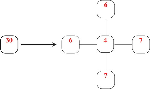
According to the calculations above, the movement of prey from cell (2, 2) to the neighbouring cells could be obtained using the function N*P_i (i = 1, 2, 3, 4, 5). The number of prey is rounded to the nearest integer. For instance, the number would stay at the same place is: N*P₁ = 30*0.126 = 3.8 ≈ 4. This movement of prey from cell (2, 2) is shown in Figure 3.

Figure 3. Move distribution of prey in cell (2, 2).

The same calculations are performed for each cell as well as for the predator population.

When all the cells and species complete their movements, the next iteration of the game is shown in Table 4. During the game movements process the total number of both species is kept the same, so at this point the total number of prey is 78, and the total number for predators is 38.

Table 4. The distribution of prey and predator (u, v) after exercising movement.

(5, 6)	(15, 9)	(7, 2)
(13, 9)	(8, 5)	(12, 2)
(5, 2)	(10, 2)	(3, 1)

2.4. Interaction function

After moving and occupying neighbouring cells, prey and predator have an interaction phase. In this case the same dynamics presented earlier [14] is utilized, using the basic model with a logistic growth function for prey and the Beddington and DeAngelis response function for the resources transfer [14–18], as shown in Equation (7).

(7) $\begin{array}{c}\frac{\mathrm{\partial }u}{\mathrm{\partial }t}=ru(1-\frac{u}{K})-\frac{auv}{b+u+cv}\\ \frac{\mathrm{\partial }v}{\mathrm{\partial }t}=\frac{eauv}{b+u+cv}-dv\end{array}$(7)

where:

u(t), v(t): the prey and predator densities at time t, respectively

r: the intrinsic growth of prey

K: the carrying capacity of prey

e: the conversion rate of prey to predator

d: the death rate of predator

a: the maximum consumption rate

b: the saturation constant

c: scales the impact of the predator interference.

Note that Equations 7 and 9 are commonly used in the literature; however, any other similar interaction function can be used in this case. This function is non-spatial and can be used to describe the interaction of predators and prey inside each cell.

Once predator and prey in each cell interact, some prey is consumed by the predators, some new prey is born and some predators die out. This step creates a new distribution of predators and prey in each cell, shown in Table 5. As shown in the table, the prey population has increased to 92 while the predator population has decreased to 33. This is the basis for the next iteration in which a new payoff is calculated, with a new probability to move and a new distribution of the species.

Table 5. The distribution of prey and predator (u, v) after interaction.

(9, 3)	(11, 4)	(9, 3)
(11, 4)	(12, 5)	(11, 4)
(9, 3)	(11, 4)	(9, 3)

3. Cross-diffusion model

This section describes the more traditional spatial cross diffusion model that is used for comparison with the game-based spatial model. This well-known model describes a phenomenon that allows predators to be aware of prey, which may affect their movement, thus helping predators to catch prey. This phenomenon – prey escape from predator and predator chase for prey, well known as cross-diffusion, has recently received substantial attention, as described in [19–22].

3.1 General cross-diffusion model

The general form of a cross-diffusion model for prey-predator interactions is

(8) $\begin{array}{c}\frac{\mathrm{\partial }u}{\mathrm{\partial }t}=f(u)-f_1(u,v)+d_{11}{\mathrm{\nabla }}^{2}u+d_{12}{\mathrm{\nabla }}^{2}v\\ \frac{\mathrm{\partial }v}{\mathrm{\partial }t}=f_2(u,v)-f(v)+d_{21}{\mathrm{\nabla }}^{2}u+d_{22}{\mathrm{\nabla }}^{2}v\end{array}$(8)

where:

f(u): birth rate function of prey

f(v): death rate function of predator

f₁(u,v): interaction function effect on the decrease of prey

f₂(u,v): interaction function effect on the increase of predator

d₁₁ and d₂₂: self-diffusion coefficients of prey and predator, respectively

d₁₂ and d₂₁: cross diffusion coefficients of predator and prey, respectively.

The value of d₁₂ and d₂₁ may be positive, negative, or zero: A positive value represents that the prey or predator move to the area that has lower concentration of another species. A negative value directs that prey or predator tends to the area that has higher concentration of another species.

3.2. Cross-diffusion model with Beddington–DeAngelis function response

Here, the basic model Equation (7) presented earlier with Beddington–DeAngelis function response and the logistic growth function for prey is extended to include the cross-diffusion effect. The corresponding model is shown below:

(9) $\begin{array}{c}\frac{\mathrm{\partial }u}{\mathrm{\partial }t}=ru(1-\frac{u}{K})-\frac{auv}{b+u+cv}+d_{11}{\mathrm{\nabla }}^{2}u+d_{12}{\mathrm{\nabla }}^{2}v\\ \frac{\mathrm{\partial }v}{\mathrm{\partial }t}=\frac{eauv}{b+u+cv}-dv+d_{21}{\mathrm{\nabla }}^{2}u+d_{22}{\mathrm{\nabla }}^{2}v\end{array}$(9)

4. Model comparison

To compare the dynamic behaviour of the different approaches, a simulation under critical conditions is conducted and the models are compared.

In order to further compare the effect of the different approaches on the stability of the system, a simulation on a 100*100 grid is conducted. Figures 4–5 demonstrate the dynamics of the prey and predator as a function of the number of iterations (left hand side) and as a function of both populations (right hand side) under different stability conditions. Subfigure (a) shows the simulation when the initial distribution of prey and predator is at a stable state of 11.54 and 4.67 respectively. Subfigure (b) shows the simulation when the initial distribution for prey and predator is not at a stable state (u = 4.67 and v = 10). Subfigure (c) shows the simulation when the initial distribution for prey and predator is outside of the stable region (u = 100 and v = 34.) Figure 4 demonstrates the system performance for the game-based model and Figure 5, described the behaviour of the cross-diffusion model.

Figure 4. System performance for the game-based model.

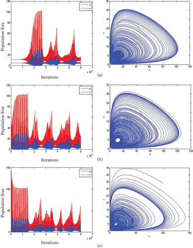
Figure 5. System performance for the cross-diffusion model.

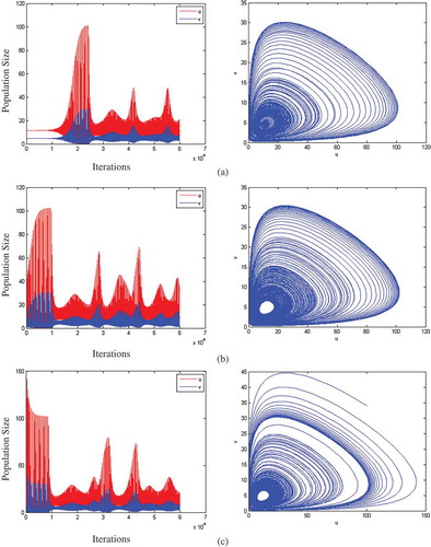
The simulation results in Figure 4 and Figure 5 show that both the game-based model and the cross-diffusion model are stable, but fluctuating. Also, the figures show that the game-based model and cross-diffusion model act similarly in different scenarios. In subfigure (a) in both modelling approaches, the prey and predator stay in the stable state and then both populations grow reaching peak point and then start to oscillate. In subfigure (b), the prey and predator populations increased to a stable state and then fluctuated in both models. In subfigure (c), prey and predator decrease to stable state and then start to fluctuate in both models.

Another comparison between the two approaches, traditional and game based is depicted in Figures 6(a–b). Here, the spatial distribution of predator and prey after 1000 iterations is compared. Unfortunately, we do not have a large scale experimental data that can be used for such a comparison.

Figure 6. (a) Distribution of the prey population on the left and predator (right) after 1000 iterations using the game model.(b) Distribution of the prey population on the left and predator (right) after 1000 iterations using the cross diffusion model.

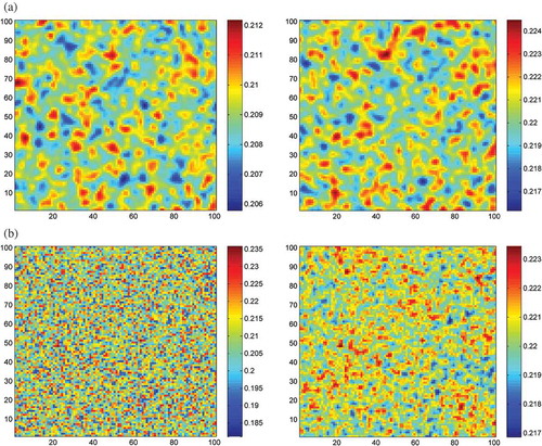
The simulation result demonstrates that the game-based model performs closely to the cross-diffusion model, indicating that the game-based model is a valid approach, although with more expressive power.

5. Model validation

This section presents an actual case with the two spotted spider mite and its predator Phytoseiulus persimilis illustrating the applicability of the game-based approach. This section describes the model’s validation using the experimental data and compares the simulated results with the actual observed data using both modelling approaches.

5.1. Background

As a species of plant-feeding mites, the two-spotted spider mite, also known as Tetranychus urticae (T. urticae), commonly considered to be a pest. Previous reports have stated that ‘T. urticae infests over 300 species of plants, including ornamental plants such as arborvitae, azalea, and viburnum, fruit crops such as blackberries, blueberries and strawberries, vegetable crops such as tomatoes, squash, eggplant, and cucumber’ [23].

Predators are beneficial in regulating spider mite population, and there are several predators that can control the spider mite populations by feeding on the adults and the eggs. Phytoseiulus persimilis (P. persimilis) is the most popular predator for this pest. This beneficial mite is commercially available and commonly released against T. urticae [24].

5.2. Experimental design

The experimental unit consisted of 24 bean plants arranged in an 8*3 array with Phytoseiulus persimilis and Tetranychus urticae as predator and prey respectively. Plants within the array were packed closely together to allow mites to move freely from plant to plant. This experiment lasted 24 days, and the total number of the two-spotted spider mites and the predator were counted every 6 days (6, 12, 18, and 24 days after the introduction of predators) during the experiment. The experiment ended after 24 days because many plants showed substantial damage and were no longer suitable hosts for the prey [25]. Table 6 lists the initial distribution of prey and predator, and Table 7 lists the total number of observed prey (Tetranychus urticae) and predator during the 24 days period.

Table 6. Initial distribution of prey and predator presented as (u,v).

(32, 6)	(0, 0)	(0, 0)
(0, 0)	(0, 0)	(0, 0)
(0, 0)	(0, 0)	(0, 0)
(0, 0)	(0, 0)	(0, 0)
(0, 0)	(0, 0)	(0, 0)
(0, 0)	(0, 0)	(0, 0)
(0, 0)	(0, 0)	(0, 0)
(32, 0)	(0, 0)	(0, 0)

Table 7. Total number of observed prey and predators every six days.

Time/Days	Number of prey	Number of predator
0	64	6
6	458	6
12	490	13
18	2238	67
24	1954	239

This data is taken from an actual study performed by the Entomology Department at Kansas State University.

5.3. Comparison of total number of prey and predator

The total number of the two-spotted spider mites and its predator were counted every six days and compared with the simulated game model and the calculated cross-diffusion model. Basic parameters for the simulation were: α = 20, b = 105, c = 45, d = 0.3, e = 0.25, r = 0.38, K = 400. While payoff parameters for the game-based model were: k₁ = k₂ = k₃ = k₄ = 100, e₁ = f = g = h = 0.01, c₁ = 0.09, c₂ = c₃ = c₄ = 100. Diffusion parameters for the cross-diffusion model were: d₁₁ = 0.01, d₁₂ = 0.005, d₂₁ = 0.001, d₂₂ = 0.03.

These parameters were chosen to create the best fit between the game-based model and the experimental data.

Figure 7 presents the comparison of the two species according to the game-based model and the observed data, and Figure 8 presents the comparison between the cross-diffusion model and the observed data. The dotted curve represents observed data, while the solid curve denotes the number of prey and predator calculated based on the simulated models. Statistical results (Root Mean Square Error) are shown in Table 8 and Table 9.

Table 8. RMSE of the simulated total number of prey and its observations.

Time/Days	Observations of prey	Model with game	Cross-diffusion
0	64	64	64
6	458	284	258
12	490	1165	781
18	2238	1982	1737
24	1954	1965	2398
RMSE		371.24	378.68

Table 9. RMSE of the simulated total number of predators and its observations.

Time/Days	Observations of predator	Model with game	Cross-diffusion
0	6	6	6
6	6	7	6
12	13	20	13
18	67	73	80
24	239	254	263
RMSE		8.82	13.42

Figure 7. Comparison of game-based model with observed data.

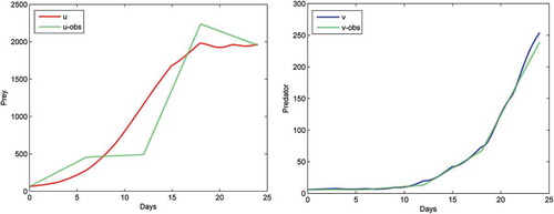
Figure 8. Comparison of cross-diffusion model with observed data.

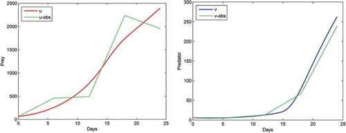
The root mean square error (RMSE) is a frequently statistical method that is used to measure the differences between predicted values by a model and the values actually witnessed. A smaller RMSE means that the model has a better fit with the data.

The detailed distribution of the predator and prey in the experiment as well as in the two models are provided in the Appendix as suggested by the reviewers.

Comparison results show that the game-based model fits the observations more closely than the cross-diffusion model since it has a smaller RMSE for both prey and predator. Thus, we conclude that the game-based model has a good fit and can generate good predictions of the prey-predator populations.

6. Conclusion and discussion

This paper presents and analyses a new modelling approach for spatial and dynamic evolutionary systems, specifically for two species prey-predator dynamics system. This new approach represents the spatial dynamics of both species as a game model which uses payoff functions that the players (the two species) can receive based on the populations in the surrounding cells. The values of the payoff for each player helps generate the probability that the players will migrate to or away from the neighbouring cells. This interaction when carried out over many iterations represents the spatial dynamics of the two species. The game-based model is simulated and compared in this paper to a more traditional cross-diffusion dynamic model that was discussed earlier. In addition to the simulation, the game-based model is validated by using actual experimental data in which the two species were observed every six days over a period of 24 days.

In the numerical simulation section, one conclusion obtained from the results was that the game-based model performed similarly to the cross-diffusion model regarding population changing, which indicates that the game-based model is a valid approach for modelling spatial-evolutionary dynamic system.

In the model validation section, the paper presents a comparison of the population of prey and predator, taking two spotted spider mites and its predator – Phytoseiulus persimilis as an example. Results show that both the game-based model and the cross-diffusion model are a good fit for the actual experimental data and the game-based model fits the observations more closely than the cross-diffusion model regarding the total number of prey and predator. Overall, we can conclude that the game-based model is a good fit and can generate good predictions of the prey-predator system.

The game-based modelling approach can be extended to other systems, such as competing commercial firms, logistic distribution systems and similar dynamic systems. The game-based approach uses a payoff function and a movement probability function that can be adjusted based on habits, characteristics and mobility schemes of different competing entities. Thus, this modelling approach can be applied to many other areas of science.

Overall, this modelling approach is more flexible and comprehensive. It can be easily extended to other systems, especially to biological and ecological dynamic systems, for instance to a virus-vector-host plant system. The game-based approach can capture complex interactions that go beyond the traditional system dynamics representation. These interactions can be modelled using the payoff functions, movement functions and other complex rules that control the interaction among the players. On the other hand, in traditional dynamic models the movement represented using a diffusion scheme is usually limited to simple movements of the players.

Future expansion of this research can include more sophisticated models, such as agent-based models [26–29] and a better tune-up of the model by using more spatial experimental data and by combining the model with the optimal control theory [30–32]. This will provide decision makers with better policies for controlling the populations of evolutionary dynamic systems.

Acknowledgements

The authors would like to thank Dr. David Margolies, and Dr. James Nechols from the Department of Entomology at Kansas State University for providing the experimental data.

Disclosure statement

No potential conflict of interest was reported by the authors.

Appendix A.

The population distribution of actual data is shown in Tables A1–A5

Table A1. Initial distribution of prey and predator presented as (u,v).

(32, 6)	(0, 0)	(0, 0)
(0, 0)	(0, 0)	(0, 0)
(0, 0)	(0, 0)	(0, 0)
(0, 0)	(0, 0)	(0, 0)
(0, 0)	(0, 0)	(0, 0)
(0, 0)	(0, 0)	(0, 0)
(0, 0)	(0, 0)	(0, 0)
(32, 0)	(0, 0)	(0, 0)

Table A2. Distribution of prey and predator presented as (u,v) on day 6.

(60, 5)	(24, 1)	(0, 0)
(14, 0)	(12, 0)	(0, 0)
(0, 0)	(0, 0)	(0, 0)
(0, 0)	(0, 0)	(0, 0)
(0, 0)	(0, 0)	(0, 0)
(0, 0)	(0, 0)	(0, 0)
(0, 0)	(0, 0)	(0, 0)
(210, 0)	(130, 0)	(2, 0)

Table A3. Distribution of prey and predator presented as (u,v) on day 12.

(52, 6)	(20, 2)	(6, 0)
(32, 0)	(8, 1)	(34, 4)
(0, 0)	(0, 0)	(0, 0)
(0, 0)	(0, 0)	(0, 0)
(0, 0)	(0, 0)	(0, 0)
(48, 0)	(22, 0)	(0, 0)
(136, 0)	(32, 0)	(0, 0)
(56, 0)	(44, 0)	(0, 0)

Table A4. Distribution of prey and predator presented as (u,v) on day 18.

(48, 2)	(12, 8)	(28, 4)
(64, 5)	(24, 9)	(76, 8)
(80, 3)	(84, 9)	(32, 6)
(76, 3)	(70, 2)	(12, 0)
(260, 6)	(76, 0)	(60, 0)
(220, 0)	(0, 0)	(368, 0)
(0, 0)	(156, 2)	(356, 0)
(0, 0)	(0, 0)	(136, 0)

Table A5. Distribution of prey and predator presented as (u,v) on day 24.

(110, 10)	(80, 24)	(98, 16)
(132, 42)	(92, 22)	(112, 26)
(124, 25)	(148, 12)	(138, 18)
(64, 8)	(88, 4)	(112, 0)
(84, 3)	(70, 3)	(116, 10)
(42, 6)	(36, 3)	(30, 1)
(24, 0)	(20, 1)	(32, 0)
(48, 2)	(72, 2)	(84, 1)

Appendix B.

The population distribution of simulated results from game-based model is shown in Tables B1–B5

Table B1. Initial distribution of prey and predator presented as (u,v).

(32, 6)	(0, 0)	(0, 0)
(0, 0)	(0, 0)	(0, 0)
(0, 0)	(0, 0)	(0, 0)
(0, 0)	(0, 0)	(0, 0)
(0, 0)	(0, 0)	(0, 0)
(0, 0)	(0, 0)	(0, 0)
(0, 0)	(0, 0)	(0, 0)
(32, 0)	(0, 0)	(0, 0)

Table B2. Distribution of prey and predator presented as (u,v) on day 6.

(7, 2)	(0, 2)	(15, 0)
(0, 2)	(30, 1)	(0, 0)
(15, 0)	(0, 0)	(0, 0)
(0, 0)	(0, 0)	(0, 0)
(0, 0)	(0, 0)	(0, 0)
(51, 0)	(0, 0)	(0, 0)
(0, 0)	(102, 0)	(0, 0)
(13, 0)	(0, 0)	(51, 0)

Table B3. Distribution of prey and predator presented as (u,v) on day 12.

(8, 1)	(1, 2)	(14, 1)
(1, 2)	(50, 2)	(0, 5)
(20, 1)	(0, 3)	(91, 1)
(1, 1)	(64, 1)	(0, 0)
(1, 0)	(241, 0)	(0, 0)
(72, 0)	(0, 0)	(371, 0)
(2, 0)	(154, 0)	(0, 0)
(19, 0)	(2, 0)	(53, 0)

Table B4. Distribution of prey and predator presented as (u,v) on day 18.

(13, 1)	(5, 2)	(14, 2)
(4, 3)	(62, 4)	(1, 8)
(23, 2)	(1, 12)	(178, 6)
(7, 2)	(78, 4)	(3, 13)
(102, 5)	(2, 1)	(536, 7)
(16, 1)	(217, 0)	(5, 0)
(58, 0)	(21, 0)	(67, 0)
(275, 0)	(239, 0)	(132, 0)

Table B5. Distribution of prey and predator presented as (u,v) on day 24.

(21, 3)	(11, 4)	(24, 3)
(10, 4)	(95, 7)	(6, 13)
(39, 4)	(5, 23)	(125, 9)
(28, 6)	(37, 9)	(22, 13)
(14, 22)	(309, 16)	(15, 37)
(139, 10)	(13, 38)	(264, 9)
(67, 12)	(210, 7)	(67, 1)
(149, 4)	(125, 0)	(170,0)

Appendix C.

The population distribution of simulated results from cross-diffusion model is shown in Tables C1–C5

Table C1. Initial distribution of prey and predator presented as (u,v).

(32, 6)	(0, 0)	(0, 0)
(0, 0)	(0, 0)	(0, 0)
(0, 0)	(0, 0)	(0, 0)
(0, 0)	(0, 0)	(0, 0)
(0, 0)	(0, 0)	(0, 0)
(0, 0)	(0, 0)	(0, 0)
(0, 0)	(0, 0)	(0, 0)
(32, 0)	(0, 0)	(0, 0)

Table C2. Distribution of prey and predator presented as (u,v) on day 6.

(64, 6)	(7, 0)	(1, 0)
(6, 0)	(0, 0)	(0, 0)
(0, 0)	(0, 0)	(0, 0)
(0, 0)	(0, 0)	(0, 0)
(0, 0)	(0, 0)	(0, 0)
(0, 0)	(0, 0)	(0, 0)
(12, 0)	(1, 0)	(0, 0)
(154, 0)	(12, 0)	(1, 0)

Table C3. Distribution of prey and predator presented as (u,v) on day 12.

(103, 10)	(37, 2)	(9, 0)
(43, 1)	(9, 0)	(1, 0)
(4, 0)	(1, 0)	(0, 0)
(0, 0)	(0, 0)	(0, 0)
(0, 0)	(0, 0)	(0, 0)
(9, 0)	(1, 0)	(0, 0)
(106, 0)	(18, 0)	(2, 0)
(314, 0)	(106, 0)	(18, 0)

Table C4. Distribution of prey and predator presented as (u,v) on day 18.

(135, 16)	(86, 9)	(47, 3)
(126, 4)	(51, 3)	(19, 1)
(39, 0)	(10, 0)	(2, 0)
(4, 0)	(1, 0)	(0, 0)
(8, 0)	(2, 0)	(0, 0)
(86, 0)	(23, 0)	(5, 0)
(270, 4)	(135, 3)	(42, 0)
(275, 22)	(239, 12)	(132, 3)

Table C5. Distribution of prey and predator presented as (u,v) on day 24.

(153, 22)	(128, 17)	(99, 12)
(155, 13)	(106, 12)	(69, 7)
(121, 5)	(56, 4)	(26, 1)
(42, 0)	(14, 0)	(4, 0)
(67, 1)	(23, 1)	(7, 0)
(167, 10)	(91, 8)	(45, 3)
(198, 23)	(165, 23)	(116, 14)
(196, 34)	(188, 30)	(162, 23)

References

- S.N. Zhao, C.H. Wu, and D. Ben-Arieh, Modeling infection spread and behavioral change using spatial games, Health Syst. 4 (1) (2015), pp. 41–53. doi:10.1057/hs.2014.22
- S. Lozano, A. Arenas, and A. Sánchez, Mesoscopic structure conditions the emergence of cooperation on social networks, PLoS ONE 3 (4) (2008), pp. e1892. doi:10.1371/journal.pone.0001892
- F.C. Santos, J.M. Pacheco, and T. Lenaerts, Evolutionary dynamcis of social dilemmas in structured heterogeneous populations, Proc Natl Acad Sci USA 103 (9) (2006), pp. 3490. doi:10.1073/pnas.0508201103
- A. Chakraborty, M. Singh, D. Lucy, and P. Ridland, A numerical study of the formation of spatial patterns in twospotted spider mites, Math. Comput. Model. 49 (2009), pp. 1905–1919. doi:10.1016/j.mcm.2008.08.013
- J.D. Murray, Mathematical Biology, 3rd ed., Springer-Verlag, Berlin, 2002.
- N. Sapoukhina, Y. Tyutyunov, and R. Arditi, The role of prey-taxis in biological control, Amer. Nat. 162 (2003), pp. 59–76. doi:10.1086/375297
- M.W. Sabelis and J.J. Van derWeel, Anemotactic responses of the predatory mite, Phytoseiulus persimilis Athias Henriot, and their role in prey finding, Exp. Appl. Acarol. 17 (1993), pp. 521–529. doi:10.1007/BF00058895
- L.S. Osborne, L.E. Ehler, and J.R. Nechols, Biological control of the twospotted spider mite in greenhouses, Bulletin (Technical), University of Florida, Cent. Fla. Res. Cent. 85 (1985), pp. 1–8.
- C.E. Van Den Boom, T.A. Van Beek, and M. Dicke, Attraction of Phytoseiulus persimilis (Acari: Phytoseiidae) towards volatiles from various Tetranychus urticae-infested plant species, Bull. Entomol. Res. 92 (2002), pp. 539–546. doi:10.1079/BER2002193
- T. Maeda and J. Takabayashi, Production of herbivore-induced plant volatiles and their attractiveness to Phytoseiulus persimilis with changes of Tetranychus urticae density on a plant, Appl. Entomol, Zool. 36 (2001), pp. 47–52. doi:10.1303/aez.2001.47
- J.G. De Boer and M. Dicke, Information use by the predatory mite Phytoseiulus persimilis (Acari: Phytoseiidae), a specialised natural enemy of herbivorous spider mite, Appl. Entomol. Zool. 40 (2005), pp. 1–12. doi:10.1303/aez.2005.1
- M. Van Wijk, P.J. De Bruijn, and M.W. Sabelis, Predatory mite attraction to herbivore-induced plant odors is not a consequence of attraction to individual herbivore-induced plant volatiles, Chem. Ecol. 34 (2008), pp. 791–803. doi:10.1007/s10886-008-9492-5
- N.F. Britton, Spatial structures and periodic travelling waves in an integro-differential reaction-diffusion population model, SIAM J. Appl. Math. 50 (1990), pp. 1663–1688. doi:10.1137/0150099
- Y. Kuang, D. Ben-Arieh, S.N. Zhao, C.H. Wu, D. Margolies, and J. Nechols, Mathematical model for two-spotted spider mites syste: verification and validation, Open J. Model. Simul. 5 (2017), pp. 13–31. doi:10.4236/ojmsi.2017.51002
- M. Haque, A detailed study of the Beddington–DeAngelis predator–prey model, Math. Biosci. 234 (2011), pp. 1–16. doi:10.1016/j.mbs.2011.07.003
- H.Y. Li and Y. Takeuchi, Dynamics of the density dependent predator–prey system with Beddington–DeAngelis functional response, J. Math. Anal. Appl. 374 (2011), pp. 644–654. doi:10.1016/j.jmaa.2010.08.029
- J.R. Beddington, Mutual interference between parasites or predators and its effect on searching efficiency, J, Animal Ecol. 44 (1975), pp. 331–340. doi:10.2307/3866
- D.L. DeAngelis, R.A. Goldstein, and R.V. O’Neill, A model for trophic interaction, Ecology. 56 (1975), pp. 881–892.
- J. Chattopadhyay and S. Chatterjee, Cross diffusional effect in a Lotka-Volterra competitive system, Nonl. Phen. Compl. Sys. 4 (2001), pp. 364–369.
- B. Dubey, B. Das, and J. Hussain, A predator-prey interaction model with self and cross-diffusion, Ecol. Modell. 141 (2001), pp. 67–76. doi:10.1016/S0304-3800(01)00255-1
- C.R. Tian, Z.G. Lin, and M. Pedersen, Instability induced by cross-diffusion in reaction-diffusion systems, Nonlinear Anal. 11 (2010), pp. 1036–1045. doi:10.1016/j.nonrwa.2009.01.043
- L. Xue, Pattern formation in a predator-prey model with spatial effect, Physica A 391 (2012), pp. 5987–5996. doi:10.1016/j.physa.2012.06.029
- T.R. Fasulo and H.A. Denmark, Twospotted Spider Mite, Featured Creatures, University of Florida Institute of Food and Agricultural Sciences, Gainesville, 2009.
- S. Wainwright-Evans, Spider mites: Stop the Spots, Interiorscape. September October (2005), pp.57-58.
- P. Nachappa, D. Margolies, J. Nechols, and J. Campbell, Variation in predator foraging behaviour changes predator–prey spatio-temporal dynamics, Funct. Ecol. 25 (2011), pp. 1309–1317. doi:10.1111/j.1365-2435.2011.01892.x
- R. Axelrod, The Complexity of Cooperation: Agent-Based Models of Competition and Collaboration, 1st ed., Princeton University Press, New Jersey, 1997.
- C.H. Wu, D. Ben-Arieh, and Z.Z. Shi, An autonomous multi-agent simulation model for acute inflammatory response, Int. J. Artif. Life Res. 2 (2) (2011), pp. 105–121. doi:10.4018/jalr.2011040106
- Z.Z. Shi, J. Wu, and D. Ben-Arieh, Agent-based model: a surging tool to simulate infectious diseases in the immune system, Open J. Model. Simul. 2 (1) (2014), pp. 12–22. doi:10.4236/ojmsi.2014.21004
- Z.Z. Shi, S.K. Chapes, D. Ben-Arieh, and C.H. Wu, An agent-based model of a hepatic in-flammatory response to Salmonella: a computational study under a large set of experimental da-ta, PLoS ONE 11 (2016), pp. e0161131. doi:10.1371/journal.pone.0161131
- W.H. Fleming, Deterministic and Stochastic Optimal Control, Springer, New York, 1975.
- S.N. Zhao, Y. Kuang, C.H. Wu, and D. Ben-Arieh, Zoonotic visceral leishmaniasis transmission: modeling, backward bifurcation, and optimal control, J. Math. Biol. 73 (2016), pp. 1525–1560. doi:10.1007/s00285-016-0999-z
- L.M. Ribas, V.L. Zaher, and H.J. Shimozako, Estimating the optimal control of zoonotic visceral leishmaniasis by the use of a mathematical model, Sci. World J. 13 (2013), pp. 810380.