Bond graph modelling of a 4-parameter photovoltaic array

ABSTRACT

A new model for simulating photovoltaic (PV) systems is presented. Bond Graph modelling is used as a basis technique. The proposed model allows prediction of generated energy under nonstandard conditions of temperature and irradiance. The proposed model is based on a 4-parameters model of the equivalent circuit of one diode. The proposed model has the property of being able to simulate the behaviour of a given PV module based only on information provided in the manufacturer datasheet. The proposed model also allows studying the effect of partial shading. As an advantage over other existing models of PV systems, the proposed model presents an extensive interconnection capacity. This feature allows simultaneous simulation with other subsystems to study the overall operation. For purposes of experimental validation of the proposed model, the construction of a $V-I$ tracer based on MOSFET that acts as a variable load is performed. The hardware control and reading of the curves are made using a data acquisition board.

KEYWORDS:

• Bond graph
• photovoltaic
• PARTIAL shading
• V – I curve
• simulator

1. Introduction

In recent decades, the study of alternative ways to generate electricity has been emphasized. There are several reasons for this, but the most notable is the concerning the climate change as a result of the excessive burning of fossil fuels. In the set of the so-called clean energies, PV generation is among the most developed. As an example of the importance of this form of energy, in Germany, about 40 TWh were generated in the year 2017 [1].

The development of PV technology has been helped by the existence of various modelling and simulation platforms. As an emerging area, photovoltaic technology has the disadvantage concerning the high monetary cost of installation. For this reason, the support received by models and simulators is vital, as these allow anticipating technical aspects of operation before purchasing a given PV plant, for only a small fraction of the cost.

There exist several ways to model a photovoltaic system. Modelling of a photovoltaic cell can be done at a detailed level in semiconductor physics, including phenomena such as density of charge carriers, carrier mobility and recombination in the charge space [2]. Such a modelling is difficult to perform by using analytical approaches, and numeric processing must be conducted to carry out simulations. It implies the requirement of high computing power. Such modelling is, however, useful and necessary for researchers who are developing new photovoltaic cells. For engineers interested in the applications of photovoltaic cells, however, such detailed modelling is not required. There exist empirical models based on measurements that are capable of estimating energy generation and anticipating efficiency [3, 4]. This form of modelling has the drawback of requiring the previous operation of the physic array. A compendium of various types of empirical modelling can be found in [5]. In many cases, a model that can reproduce entirely or partially the $V-I$ curve of the solar array under given conditions is sufficient. This curve is used to predict the power that the array can provide. Different approaches are used for this. Some methods predict some points of the $V-I$ curve, such as the Sandia performance model, which defines five points, including the maximum power point [6]. Other modelling methods can predict the entire curve. In this type, the one diode and two diodes equivalents are widely used as modelling methods. Depending on the chosen equivalent, groups of three or more parameters are required [7]. The method to calculate these groups of parameters varies among authors. Indeed analytical methods, iterative methods, and artificial intelligence algorithms have been used. A more detailed review of these equivalents can be found in [7] and [8]. Among the analytical methods for the calculation of the parameters, the one presented in [9] allows calculating five parameters from information contained in the datasheet of the module under analysis. Such an approach is attractive, as no previous testing or measurements are required. This paper uses the equivalent of one diode with a series resistor, which involves four parameters [7]. The calculation of the parameters is done analytically based on an approach presented in [10]. Explicit expressions which avoid the iterative techniques required by other methods are used. This method allows the proposed model to have sufficient accuracy and computation speed. Besides, the calculation of the four parameters is also derived from information contained in the datasheet.

Electric power generation is a process that involves conversion between different energy domains. The electrical energy is usually not obtained as such, but it is necessary to perform a transformation in places where the primary form of energy can be thermal, mechanical, chemical, nuclear, radiant, etc. Once generated, power is transmitted to areas of consumption where the reverse process takes place, that is, it should be converted to the form of final energy of interest, which may be thermal, mechanical, radiant, chemical, etc. This aspect of conversion between different energy domains is one of the most attractive characteristics of the Bond Graph modelling [11]. Indeed, within a Bond Graph, a system composed of subsystems belonging to different engineering areas can be represented in the same context [12]. Thus, power generation modelling is suitable to be made by Bond Graphs. In particular, Bond Graph modelling is very suitable for the PV generation systems studied in this paper. In addition to its multi-domain nature, another attractive feature of Bond Graphs is causality. By analysing causality, it is possible to mathematically determine whether a system element responds directly as a result of action taken in another system element [13].

Another advantage of using this methodology is the existence of software capable of performing simulations of systems modelled as Bond Graphs.

A problem of PV systems is the shadow projection on some sections of the modules. This issue is known as partial shading. Three major consequences occur as a result of the partial shading: First, the total power output of the plant decreases significantly [14]. Second, forced reverse bias in shaded sections causes excessive current flows which in turn originate hot spots that can damage the module [15]. Third, the traditional techniques for maximum power point tracking (MPPT) may fail, by following to false local peaks [16]. The study of the effect of shading is still subject to discussion and research. Proper installation of bypass diodes, distribution arrangements to minimize losses from partial shading, as well as to develop better MPPT techniques are issues that require further observation and study. This paper presents a model of PV systems capable of representing the effect of partial shading on an arbitrary number of sections of a given array. The proposed model can be an aid in the study of the effects of partial shading and the development of new MPPT techniques that take into account this problem.

The modelling of PV systems can be divided into two areas, according to the application. First, a PV model can be used as a tool to predict the power output in a given period and location. Second, it can be used as a simulator of the behaviour of an actual PV system for the development and improvement of related subsystems. In the latter case, the model can be used to study power electronics converters, effects of grid interconnection, MPPT strategies, effects of interconnection with other energy sources such as wind generators, etc. For these purposes, the model must be able to interconnect with all the other subsystems. Several developed models are focused on estimate energy production, or to conduct a study on economic aspects [5]. However, few models can incorporate other submodels through interconnection [17]. Moreover, by forcing the solution of a predefined set of equations, some proposed alternatives lose the characteristic of modularity [18].

The mathematical part of the model presented in this paper is analytical and explicit, which makes it light in simulation. The model is Bond Graph based and therefore allows to preserve topological properties. As a result, the interconnection with other subsystems is performed naturally. The model can be constructed with information contained in the data sheets. Also, a photovoltaic system can consist of a large section with consistent behaviour, or with many sections with different behaviours due to mismatch and partial shading. All existing methods can deal with the first case. However, Bond Graph allows dealing with the second instance also in a natural way.

The remainder of the paper is organized as follows: In Section 2, the Bond Graph model of photovoltaic arrays is presented. In Section 3, some experiments are summarized in order to give practical validity to the proposed model. First, a comparison between the 4-parameter model and a 5-parameter model is performed. Then a comparison between the curves predicted by the model and those measured experimentally in a real module is made. Also, the interconnection capacity of the proposed model is shown by using the proposed model as a source for a DC motor and a MPPT controller. Finally, in Section 4 some final comments and conclusions of the paper are written. The notation can be consulted in the appendix.

2. Bond graph model of a PV system

2.1. Basics of bond graph modelling

The Bond Graphs introduced by Henry Paynter [19] constitute a useful modelling technique. The fundamental element is the bond, which functions as a link between two elements that exchange energy. Through this essential element, power is transferred between the two items that are interconnected by it. This transfer is done by sharing two variables associated with each bond whose mathematical product is power. The variables that intervene are called generalized effort and flow. These variables can be part of several physical domains. Table 1 summarizes the meaning of the generalized variables in some physical areas.

Table 1. Generalized variables.

Domain	Effort	Flow
Translational	Force	Velocity
Rotational	Torque	Angular speed
Electric	Voltage	Current
Hydraulic	Pressure	Flow rate

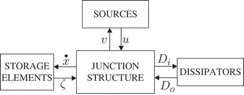
The underlying idea of modelling a Bond Graph is to consider that a physical system consists of external components or subsystems and the necessary information regarding how they interconnect and exchange energy with each other. Figure 1 shows the block diagram of a Bond Graph.

Figure 1. Fields that form a causal bond graph model.

Figure 1 shows the fields and the key vectors in a Bond Graph. $\stackrel{\bullet }{x(t)}$ is the vector of state variables. $\zeta (t)$ is the vector of co-energy variables. $u(t)$ is the vector of inputs to the system and $v(t)$ is its complement. $D_i(t)$ and $D_o(t)$ are the vectors of generalized variables directed to and from the dissipative field, respectively. Mathematically,

$\left[\begin{array}{c}\stackrel{\bullet }{x}\\ D_i\end{array}\right]=\left[\begin{array}{ccc}{S}_{11}& S_{12}& S_{13}\\ S_{21}& S_{22}& S_{23}\end{array}\right]\left[\begin{array}{c}\zeta \\ D_o\\ u\end{array}\right]$

$S$ is called the junction structure matrix.

The source block consists of the external components that supply power. The storage block consists of the components capable of storing energy. The dissipator block consists of elements that dissipate energy. The central block, called the junction structure corresponds to the information on how the components are interconnected. 0-junctions, 1-junctions, transformers, and gyrators are part of it and together determine the topology of the modelled system. This junction structure is energy conservative and if a zero input is applied, and if all the storage elements accept integral causality, then the key vectors satisfy,

(1) $0=\stackrel{{\bullet }^T}{x}\zeta +D_i{D}_o$(1)

Where$\stackrel{{\bullet }^T}{x}\zeta$ and $D_i{D}_o$ are the stored and dissipated energy, respectively. Equation (1) is equivalent to

(2) $0={\zeta }^T{S}_{11}^T\zeta +D_o^T{S}_{12}^T\zeta +{\zeta }^T{S}_{21}^T{D}_o+D_o^T{S}_{22}^T{D}_o$(2)

Since the first and last terms of Equation (2) are zero when $S_{11}$ and $S_{22}$ are skew-symmetric matrices, then, from Equation (2), an energy-conservative system satisfies the properties,

$S_{11}$ and $S_{22}$ are skew-symmetric matrices, and

$S_{12}=-S_{21}^T$

If a bond binds an element of the junction structure to one of any other of the blocks, it is called an external bond. It is referred to as an internal bond in another case.

The 0/1 junctions allow coupling two or more elements that are subject to a unique effort/flow. In these junctions, the flow/effort obeys Kirchhoff’s law of currents/voltages, in such a way that at junctions with $n$ incident bonds

$f_1+f_2+...+f_n=0$ in 0-junctions, and

$e_1+e_2+...+e_n=0$ in 1-junctions stands.

The energy sources can have flow or effort as their primary variable. This variable is independent, while the other variable depends on the nature of the system to which the source is interconnected.

The storage elements maintain constitutive relationships that relate effort to flow through non-linear functions for the general case. Although in many models it is useful to establish only linear relationships.

Energy-dissipating elements also show a non-linear function in the general case that relates effort to flow. Similarly to storage elements, dissipators often use a linear constitutive relationship. For example, consider Shockley’s equation for diodes, mentioned later in this paper and Ohm’s Law. Both expressions relate voltage to the current through a mathematical expression. However, the former does it non-linearly, while the other does it linearly.

Causality is a concept that plays a significant role in Bond Graphs. It establishes in each element which variable is considered as independent and which is the dependent one. By visual inspection of the causal paths, it is possible to verify various properties of the system, before any mathematical treatment. By analysing causality, the formulation of equations becomes a methodical and straightforward procedure. The most commonly used method to establish causality in a Bond Graph is the sequential causality assignment procedure (SCAP).

Bond Graph modelling is a mature technique that is widely documented. The uninitiated reader is encouraged to consult references such as [11] to go deeper into the theoretical basis.

2.2. Bond graph model of a photovoltaic array

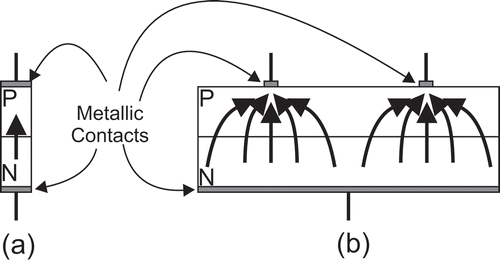
The construction of a PV cell consists in the union of a P-type semiconductor material with an N-type, similarly as occurs in a diode [7]. However, unlike the latter, where it can be considered that the electron current describes a simple trajectory, in the photovoltaic cell, there is a large contact surface between the two regions, resulting in the existence of many current paths, as shown in Figure 2.

Figure 2. Distributed current trajectories in a PV cell.

It can be seen in Figure 2 that the upper metallic contacts should be ample to allow proper flow of current, but must also be small to obstruct the least possible amount of incident light into the union.

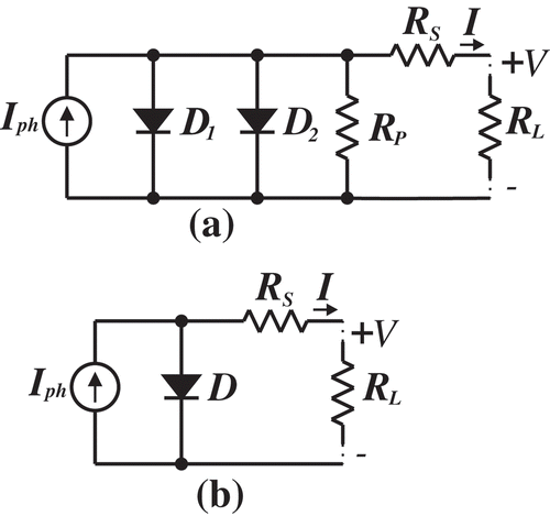
By analysing Figure 2, an appropriate way to model a photovoltaic cell consists of its representation through uniformly distributed diodes [20]. However, a representation of this kind is difficult to assess computationally and should be chosen only when extreme accuracy is required. A simpler representation preserving a good degree of precision consists of two diodes arranged as shown in Figure 3(a).

Figure 3. (a) Two-diode equivalent. (b) One-diode equivalent with a series resistor.

In the model of Figure 3(a), the current source $I_{ph}$ denotes the current generated by the influence of incident light and is commonly called photocurrent. The parallel resistance $R_p$ represents recombination losses, and the series resistance $R_s$ represents losses by contact and metallization. Diode $D_1$ denotes the effect of charge diffusion, and diode $D_2$ symbolizes the effect of the charge recombination in the space-charge PN layer [21]. The load resistance $R_L$ allows to visualize the interconnection of the array, but it is not part of the model.

To mathematically model the circuit of Figure 3(a), it is necessary to calculate seven parameters. Different methods for estimating these parameters are found in the literature. In this paper, however, the equivalent of Figure 3(b), in which the diode $D_2$ has been removed, is used. This diode represents the phenomenon of charge recombination, which has a negligible effect under conditions of high irradiance. The resistor $R_p$ has also been removed. The presence of this resistor has a negligible effect at high irradiance, even in low irradiance, it influences with less than 5% in the difference in the maximum power. Besides, the equivalent of Figure 3(b) requires only four parameters.

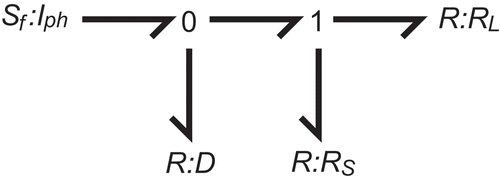
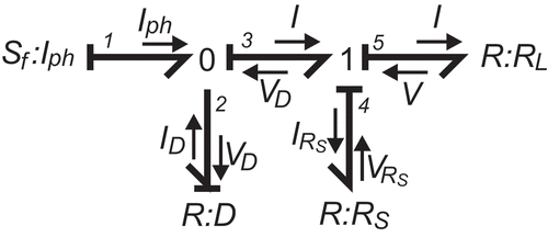
The circuit of Figure 3(b) is the basis of the model proposed in this paper. It is well known that an electric circuit can be converted directly to a Bond Graph [11]. If the circuit of Figure 3(b) is converted to its Bond Graph equivalent, then the model of Figure 4 is obtained.

Figure 4. Bond graph of the one diode equivalent circuit.

In Figure 4, the photocurrent source is assigned a value which depends on the incident irradiance and temperature. The diode is modelled by a resistor whose constitutive relation is the well-known Shockley equation [22]:

(3) $I_D=I_0\left(exp\left(\frac{q}{nk{T}_C}{V}_D\right)-1\right)$(3)

Where $I_0$ is the reverse saturation current of the diode, $q$ is the electron charge, with a value $q=1.602\times {10}^{-19}C$, $n$ is the diode ideality factor, $k$ is the Boltzmann constant with a value $k=1.381\times {10}^{-23}J/K$, and $T_C$ is the temperature of the device expressed in Kelvins. As this relation is non-linear, this element must preserve conductance causality to avoid numerical issues. The value of the resistance $R_s$ is one of the four parameters to be calculated as shown below. Once calculated, its value remains fixed. This element behaves as a normal resistance and can accept any causality. The $R_L$ element acts as a load to the array. At this port, any other Bond Graph model can be interconnected.

The Bond Graph of Figure 4 is the fundamental block of the proposed model. Within a more complex model, several instances of such a fundamental block can be incorporated. Each instance can have separate irradiance and temperature inputs, allowing the model to reproduce the shading phenomena of sections of an array wherein the irradiance is not uniform. It is also possible to model the effect of temperature variations in different sections of the array. The main difficulty in the proposed model consists of calculating certain parameters that are fundamental in the formulation of the descriptive equations. The formulation of the mathematical model of Figure 4 is a central theme, and it is presented in the following subsection.

2.3. Calculation of the four parameters of the model

In Figure 5, the Graph of Figure 4 has been redrawn. The causality has been assigned, and the Bonds have been labelled.

Figure 5. Bond graph model of a PV system with assigned causality.

In the Bond Graph of Figure 5, the 0-junction has the following constitutive relation:

(4) $I=I_{ph}-I_D$(4)

where $I_D$ is the diode current, represented as a function of the diode voltage $V_D$, by Equation (3), which is rewritten as:

(5) $I_D=I_0\left(exp\left(\mathrm{\Lambda }{V}_D\right)-1\right)$(5)

with

(6) $\mathrm{\Lambda }=\frac{q}{nk{T}_C}$(6)

Is worth noting that the parameter $n$ is no longer visible, but it is contained within the expression for $\mathrm{\Lambda }$.

In Figure 5, the constitutive relation in the 1-junction is:

$V_D=V_{R_S}+V$

as $R_S$ has a linear behaviour, then $V_{R_S}=R_{S}I$ and

(7) $V_D=R_{S}I+V$(7)

By substituting Equation (7), into Equation (5), then Equation (4) can be written as:

(8) $I=I_{ph}-I_0\left(exp\left(\mathrm{\Lambda }\left(R_{s}I+V\right)\right)-1\right)$(8)

Equation (8) determines a non-linear implicit 4-parameter model [5]. The set of four parameters $\left\{I_{ph},I_0,R_s,n\right\}$ allows the characterization of the $V-I$ curve of a given PV cell.

The following information is required as input to the computation of the four parameters: short-circuit current $I_{SC}$, open circuit voltage $V_{OC}$, maximum power voltage $V_{MP}$ and maximum power current $I_{MP}$. The data set $\left\{I_{SC},V_{OC},V_{MP},I_{MP}\right\}$ will be named $D_{in}$ along the paper. If $D_{in}$ is available, Equation (8), which corresponds to the $V-I$ curve can be known in three points. First, considering the point of short-circuit current, where $I=I_{SC}$ and $V=0$, then Equation (8) can be written as:

(9) $0=-I_{SC}+I_{ph}-I_0\left(exp\left(\mathrm{\Lambda }{R}_s{I}_{SC}\right)-1\right)$(9)

Now, considering the point of open circuit voltage, it follows that $I=0$ and $V=V_{OC}$ and Equation (8) can be written as:

(10) $0=I_{ph}-I_0\left(exp\left(\mathrm{\Lambda }{V}_{OC}\right)-1\right)$(10)

The third point of the curve may be known under conditions of maximum power, where $I=I_{MP}$ and $V=V_{MP}$. Then, Equation (8) is written as:

(11) $0=-I_{MP}+I_{ph}-I_0\left(exp\left(\mathrm{\Lambda }\left(R_s{I}_{MP}+V_{MP}\right)\right)-1\right)$(11)

Equations (9)–(11) are in terms of the four parameters $I_{ph}$, $I_0$, $R_s$ and $n$. To form a system of four equations with four unknowns, it becomes necessary to build the fourth equation. It is constructed from the voltage-power curve in which at the maximum power point, the derivative is zero, according to:

(12) $\frac{dP}{dV}=V\frac{dI}{dV}+I\frac{dV}{dV}=0$(12)

Calculating the derivative $\frac{dI}{dV}$ of the current, given by Equation (8), substituting into Equation (12) and considering the current and voltage values at the maximum power point, by algebraic manipulation the fourth equation is obtained:

(13) $0=I_{ph}+I_0-I_{0}exp\left(\mathrm{\Lambda }\left(V_{MP}+I_{MP}{R}_s\right)\right){\mathrm{\Theta }}_1$(13)

with ${\mathrm{\Theta }}_1=1+\frac{\mathrm{\Lambda }{V}_{MP}}{1+I_0\mathrm{\Lambda }{R}_{s}exp\left(\mathrm{\Lambda }\left(V_{MP}+I_{MP}{R}_s\right)\right)}$

Equations (9), (10), (11) and (13) form a system of four equations with four unknowns, which can be solved by computer numerical methods, or explicitly, by using some simplifications, as is shown below and done in [10].

From Equation (9), considering that the voltage drop at the series resistor $R_{s}I$ is tiny, it can be neglected, and it leads to:

(14) $0\approx -I_{SC}+I_{ph}$(14)

In Equation (10), the $-1$ term can be neglected without significantly affecting the relationship because the value of $V_{OC}$ in the exponential term is greater than one by several orders of magnitude. By removing that term, it is:

(15) $0\approx I_{ph}-I_{0}exp\left(\mathrm{\Lambda }{V}_{OC}\right)$(15)

In Equation (11), it is possible to do the same simplification, as, at the value of maximum power, the exponent is large. The simplification can be written as:

(16) $0\approx -I_{MP}+I_{ph}-I_{0}exp\left(\mathrm{\Lambda }\left(R_s{I}_{MP}+V_{MP}\right)\right)$(16)

Equations (14)–(16) are part of a new simplified system. Before considering the fourth equation of this new system some results can be anticipated. According to Equation (14) the photocurrent can be expressed as:

(17) $I_{ph}\approx I_{SC}$(17)

Substituting Equation (17) into Equation (15) and solving for $I_0$, it leads to:

(18) $I_0\approx \frac{I_{SC}}{exp\left(\mathrm{\Lambda }{V}_{OC}\right)}$(18)

In addition, using a similar reasoning as made in the simplification which led to Equations (15) and (16), Equation (8) can be written as:

(19) $I\approx I_{ph}-I_{0}exp\left(\mathrm{\Lambda }\left(R_{s}I+V\right)\right)$(19)

Substituting Equations (17) and (18) into Equation (19) it leads to:

(20) $I\approx I_{SC}\left(1-exp\left(\mathrm{\Lambda }\left(R_{s}I+V-V_{OC}\right)\right)\right)$(20)

Then the conditions to calculate the fourth equation are met, using the maximum power point in the $V-P$ curve. For this, the derivative of the current (20) is calculated with respect to the voltage, according to:

(21) $\frac{dI}{dV}\approx \frac{-I_{SC}\mathrm{\Lambda }exp\left(V+I{R}_s-V_{OC}\right)}{1+I_{SC}\mathrm{\Lambda }{R}_{s}exp\left(V+I{R}_s-V_{OC}\right)}$(21)

Substituting Equations (20) and (21) into Equation (12) and considering the values of current and voltage at the maximum power point $I_{MP}$ and $V_{MP}$ it leads to:

(22) $0\approx 1-exp\left(\mathrm{\Lambda }\left(V_{MP}+I_{MP}{R}_s-V_{OC}\right)\right){\mathrm{\Theta }}_2$(22)

with ${\mathrm{\Theta }}_2=1+\frac{\mathrm{\Lambda }{V}_{MP}}{1+I_{SC}\mathrm{\Lambda }{R}_{s}exp\left(\mathrm{\Lambda }\left(V_{MP}+I_{MP}{R}_s-V_{OC}\right)\right)}$.

Substituting Equations (17) and (18) into Equation (16) the following is obtained:

(23) $0\approx -I_{MP}+I_{SC}\left(1-exp\left(\mathrm{\Lambda }\left(V_{MP}+I_{MP}{R}_s-V_{OC}\right)\right)\right)$(23)

Solving for $R_s$ in Equation (23) it leads to:

(24) $R_s\approx \frac{1}{I_{MP}}\left(\frac{ln\left(\frac{I_{SC}-I_{MP}}{I_{SC}}\right)}{\mathrm{\Lambda }}-V_{MP}+V_{OC}\right)$(24)

Substituting Equation (24) into Equation (22) and solving for $\mathrm{\Lambda }$, it leads to:

(25) $\mathrm{\Lambda }\approx \frac{\frac{I_{MP}}{I_{SC}-I_{MP}}+ln\left(1-\frac{I_{MP}}{I_{SC}}\right)}{2V_{MP}-V_{OC}}$(25)

Equation (25) is fundamental, as its solution allows calculation of the necessary parameters. If Equation (6) is solved for $n$ the last parameter can be calculated, according to:

(26) $n=\frac{q}{\mathrm{\Lambda }k{T}_C}$(26)

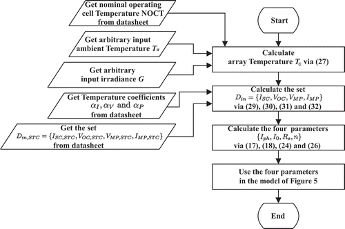
Summarizing, given the data set $D_{in}$, using Equations (17), (18), (24) and (26) the four parameter set $\left\{I_{ph},I_0,R_s,n\right\}$ can be obtained.

The system formed by Equations (9), (10), (11) and (13) has the disadvantage of being implicit and requires a specialized solver that can present numerical issues. In counterpart, the system formed by Equations (17), (18), (24) and (26) is explicit, and a solution can always be expected. The four parameters calculated by the two methods present a negligible difference. Table 2 shows the results obtained by both methods for a Canadian Solar CS6P-255P solar panel with a temperature of ${25}^{\circ }C$ and two different irradiances. The maximum relative error of the generated power is also shown.

Table 2. Calculated values for the four parameters.

	$G=1000W/m^2$		$G=100W/m^2$
	Implicit	Explicit	Implicit	Explicit
$I_{ph}$	$9.0$	$9.0$	$0.9$	$0.9$
$I_0$	$2.8743\times {10}^{-8}$	$2.8744\times {10}^{-8}$	$2.8738\times {10}^{-9}$	$2.8744\times {10}^{-9}$
$R_s$	$0.2283$	$0.2283$	$2.283$	$2.2829$
$n$	$74.4129$	$74.4130$	$74.4122$	$74.4130$
Error	$1.415\times {10}^{-6}$		$1.085\times {10}^{-6}$

2.4. Temperature model

An accepted way of modelling the temperature in solar panels is based on the nominal operating cell temperature (NOCT) [23]. Furthermore, the manufacturer also provides this information. According to this criterion, the array temperature $T_C$ can be calculated as a function of the nominal operating cell temperature of the cell $NOCT$, the ambient temperature $T_a$ and the irradiance $G$ as [24]:

(27) $T_C=T_a+\frac{NOCT-20}{800}G$(27)

In this way, the model described below can either accept the ambient temperature $T_a$ or the temperature of operation $T_C$ directly, in which case, Equation (27) must convert it.

2.5. Scaling parameters to current operating conditions

We will name $D_{in,STC}$ the $D_{in}$ set when it operates under standard test conditions (STC). Under these circumstances, the array temperature is ${25}^{o}C$, the irradiance is $1000W/m^2$, and an air mass of $1.5$ is considered. Manufacturers only provide the set $D_{in,STC}$. In addition to the set $D_{in,STC}$, the proposed model requires more information that also is supplied in the datasheet. These data are the open circuit voltage temperature coefficient ${\alpha }_V$, the short circuit current temperature coefficient ${\alpha }_I$ and the maximum power temperature coefficient ${\alpha }_P$.

To know the set $D_{in}$ at arbitrary irradiance $G$ and array temperature $T_C$, it is necessary to scale the set $D_{in,STC}$ to the required conditions.

First, the photocurrent $I_{ph}$ can be calculated as a linear function of the irradiance, with an included temperature adjustment according to [23]:

(28) $I_{ph}=I_{ph,STC}\frac{G}{G_{STC}}\left(1+{\alpha }_I\left(T_C-T_{C,STC}\right)\right)$(28)

where $G_{STC}$ and $T_{C,STC}$ are irradiance and temperature under standard test conditions. According to Equation (17), the short circuit current in the new operating conditions can be approximated by:

(29) $I_{SC}=I_{SC,STC}\frac{G}{G_{STC}}\left(1+{\alpha }_I\left(T_C-T_{C,STC}\right)\right)$(29)

The open circuit voltage $V_{OC}$ is scaled directly by the coefficient of variation of voltage ${\alpha }_V$ by:

(30) $V_{OC}=V_{OC,STC}\left(1+{\alpha }_V\left(T_C-T_{C,STC}\right)\right)$(30)

Manufacturers typically do not provide a coefficient of variation of the maximum power voltage. However, a technique for tracking the maximum power point assumes that the percentage of change of the open circuit voltage versus the maximum power voltage is almost constant [25]. This assumption can be considered to use the same coefficient ${\alpha }_V$ when calculating the maximum power voltage $V_{MP}$ according to:

(31) $V_{MP}=V_{MP,STC}\left(1+{\alpha }_V\left(T_C-T_{C,STC}\right)\right)$(31)

For the calculation of the maximum power current, the already calculated maximum power voltage can be used. First, the power temperature coefficient ${\alpha }_P$ is used to calculate the maximum power by:

(32) $P_{MP}=P_{MP,STC}\frac{G}{G_{STC}}\left(1+{\alpha }_P\left(T_C-T_{C,STC}\right)\right)$(32)

Equation (32) is a function of the array temperature $T_C$, as well as of the irradiance $G$. In addition to the correction for temperature given by ${\alpha }_P$, the $G/G_{STC}$ scaling is required because it is assumed that the relationship between maximum power and irradiance is linear [26]. Then the maximum power current can be calculated by:

(33) $I_{MP}=\frac{P_{MP}}{V_{MP}}$(33)

In this way, the set $D_{in}$ is obtained based on the new conditions of irradiance and temperature and can be used to calculate the four parameters. To summarize, in Figure 6 the flow diagram to get the parameters is shown.

Figure 6. Flow diagram to get the four parameters.

2.6. Implementation of the proposed model

In the Bond Graph of Figure 4, the $I_{ph}$ flow source must be provided with the irradiance $G$ and the array temperature $T_c$, so that $I_{ph}$ can be calculated by Equation (28). The constitutive relation of the resistive element corresponding to the diode is the Shockley Equation (3). Due to the nature of such constitutive relation, this element must remain in conductance causality. This resistive element also requires as input the temperature value $T_c$. The value of the series resistance is calculated by Equation (24).

The set $D_{in,STC}$ of conditions provided in the datasheet corresponds to a complete panel consisting of $n_s$ cells in series. Therefore, the $D_{in}$ set calculated from $D_{in,STC}$ also corresponds to an entire panel. However, commercial panels are constructed by several sections of $n_{se}$ cells in series protected by a bypass diode. It is necessary to scale part of the $D_{in}$ set to calculate the ${D_{in}}^{\prime }$ set corresponding to each subsection. Specifically, Equations (30), (31) and (32) must be multiplied by the scaling factor $n_{se}/n_s$.

In particular, a scaling of $1/n_s$ allows obtaining the model of a single cell. This model can be used as a fundamental block to build complex photovoltaic arrays, but this is not recommended as numerical problems could be introduced. It is advisable to keep the number of equations in the minimum possible that each simulation requires.

The proposed model can be implemented in software capable of handling Bond Graphs. For test purposes in this paper, the 20sim programme has been chosen [27]. By the nature of the model, however, it can be implemented in other simulation platforms. For example, it can be realized naturally in Modelica [28], since this simulation and modelling environment maintains two important characteristics in common with Bond Graphs that are essential in the model: The ability to integrate multi-domain systems and the preservation of topological properties of the modelled system. The model can also be implemented in other platforms like Matlab/Simulink, although this particular case is more complicated because the model is not intended to be managed by the most abstract blocks characteristic of that platform.

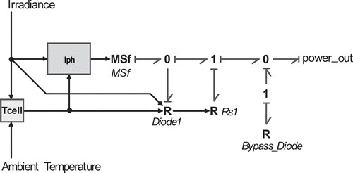
In Figure 7 the 20-sim implementation of the PV array is shown.

Figure 7. 20-sim submodel of a PV source.

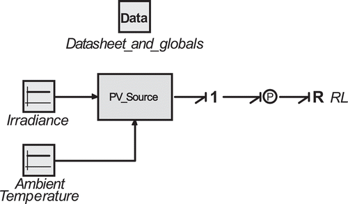
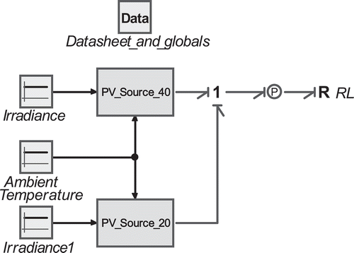
The Bond Graph of Figure 7 is implemented as a submodel consisting of two signal inputs, corresponding to the irradiance and ambient temperature. It also includes a power output where the interconnection with the load is done. In the Tcell block, the irradiance $G$ and ambient temperature $T_a$ are taken as inputs and by Equation (27) the array temperature $T_C$ is calculated. The Iph block takes as inputs the irradiance and the array temperature. In this block, the photocurrent value is computed by Equation (28). This value is used to modulate the flow source. In the resistive element corresponding to the diode, the irradiance and array temperature variables are taken as inputs. This element has the constitutive relation (3). For purposes of modularity, the Bond Graph of Figure 7 is embedded in the PV_Source submodel that can be used according to the configuration shown in Figure 8.

Figure 8. 20-sim use of the PV source.

In the Data block of Figure 8, the set $D_{in,STC}$, the temperature coefficients ${\alpha }_V$, ${\alpha }_I$, ${\alpha }_P$, the NOCT value and the number $n_s$ of cells in series in the module must be entered. Each PV_Source block represents an array with its properties. Separate instances of the PV_Source block can be connected through 0-junctions and 1-junctions to combine different arrays with different features.

After presenting the model, to verify its validity, some tests are needed. These tests are performed in the next section.

3. Model validation

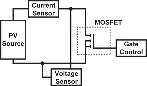
For validation of the proposed model, it is necessary to compare the curves obtained through simulations against curves obtained by measurements in a real PV array. For purposes of obtaining the $V-I$ and $V-P$ curves of a real array, the idea of employing a MOSFET as a variable load element will be exploited. This concept has already been reported before [29]. The idea is to regulate the flow of current in the device by controlling the gate voltage. Figure 9 shows a schematic of the used circuit.

Figure 9. MOSFET-based $V-I$ tracer.

The IRFP260 MOSFET is used. This device allows dissipating the power delivered by a single 250 W PV module. The 20A Hall effect sensor ACS712 is used as a current measuring device. To measure the voltage a high impedance dividing branch coupled by operational amplifier is employed. The output of the current and voltage sensors is converted into digital data by the Humusoft AD622 data acquisition board [30]. This data acquisition board can interact with MATLAB-Simulink [31] through the real time toolbox.

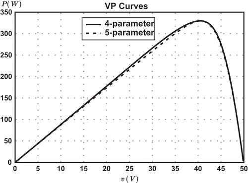
The proposed model allows simulating different configurations of arrays of PV modules. As a first test, a comparison between the set of parameters calculated by the 4-parameter explicit method (4PE) used in this paper, the 4-parameter implicit method (4PI) and the 5-parameter method (5P) proposed in [9] is performed. Table 3 shows the comparative.

Table 3. Comparison between the parameters calculated by 4-parameter methods and 5-parameter method.

Module	Method	$a\left(V\right)$	$I_{ph}\left(A\right)$	$I_0\left(A\right)$	$R_s\left(\mathrm{\Omega }\right)$
Solartec	4PE	1.86	8.74	1.859$\times {10}^{-8}$	0.19
S60MC-250	4PI	1.8679	8.74	1.858$\times {10}^{-8}$	0.19
	5P	1.628	8.745	9.672$\times {10}^{-10}$	0.2488
Canadian Solar	4PE	1.91	9	2.87$\times {10}^{-8}$	0.228
CS6P-255P	4PI	1.92	9	2.874$\times {10}^{-8}$	0.2283
	5P	1.62	9	8.36$\times {10}^{-10}$	0.2963
Kyocera	4PE	3.06	8.79	7.869$\times {10}^{-7}$	0.164
KD33GX-LFE	4PI	3.074	8.79	7.87$\times {10}^{-7}$	0.165
	5P	2.223	8.8	1.53$\times {10}^{-9}$	0.3625

The value of $a$ is considered according to [9] as

$a=\frac{nk{T}_C}{q}$

The parameters shown in Table 2 have been obtained under standard test conditions. The Figure 10 shows the comparative of the $V-P$ curves for a Kyocera KD33GX-LFE module under standard test conditions.

Figure 10. $V-P$ curve comparative between 5-parameter and 4-parameter models.

It can be seen in the curves in Figure 10 that there is virtually no difference between the 4P and 5P approaches, observing only a slight separation at intermediate not crucial points. Furthermore, as can be concluded from the results in Table 3, the difference between the curves calculated with the two 4P approaches cannot be visually appreciated, since the coincidence is too close.

For validation purposes with a real system, a Solartec S60MC-250 module is tested. This module has 60 cells connected in series. The arrangement consists of 3 sections of 20 cells each. A bypass diode protects each section. In that way, shadows can be projected over any section to study the response in these conditions. The tracer shown in 9 reads the $V-I$ and $V-P$ curves. The AD622 data acquisition card is also used to measure the temperature of the module, with LM35 sensors placed as required. Due to the lack of control in the conditions of temperature and air velocity in the tests below, the temperature model described by Equation (27) is not used, but instead, the temperature measured by the sensor is provided directly to the model as the variable $T_C$. The irradiance is measured with the TES-1333 m. Readings are performed under the following conditions: with the module covered at rest, it is suddenly exposed to sunlight. 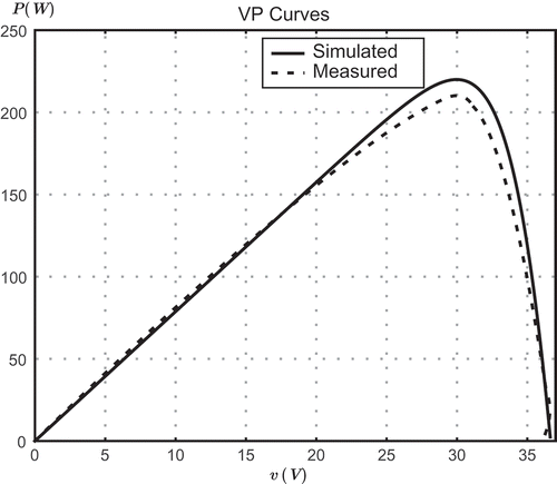Then measurements of $V-I$ and $V-P$ curves are carried out simultaneously with the measurement of irradiance. Then the module temperature measurement is performed. This procedure prevents the panel from overheating, allowing monitoring of higher power output. A first test consists of exposing the entire module to uniform irradiance conditions. In the test, an irradiance in the plane of the array of $890$ $W/m^2$ and a module temperature of ${30}^{o}C$ are measured. In Figure 11, a comparative of the measured curve against the simulated curve is shown.

Figure 11. $V-P$ Curves.

The curves in Figure 11 show an acceptable correspondence with an estimated error of 3.01%. The measured curve shows a maximum power point below the predicted by simulation. This difference may be due to several factors, including irregularities in the construction of the module or inaccuracy in measuring irradiance. Moreover, the measured curve shows an irregularity near to the point of $V_{OC}$. This anomaly is due to the MOSFET-based method of reading the curve.

In a second test, the effect of shading on a section of the module can be observed. In this test, a whole cell is placed under the shade, as shown in Figure 12.

Figure 12. Photovoltaic module with partial shading.

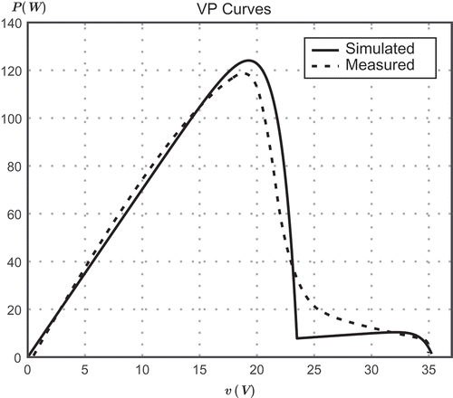
The shaded cells form part of an individual section protected by a bypass diode, while other two sections are formed with the cells exposed to light. The simulation is performed by the instantiation of two sections, one of 20 cells subjected to the measured average irradiance of $145W/m^2$ and another of 40 cells subjected to an irradiance of $810W/m^2$. Figure 13 shows this configuration.

Figure 13. Two instances of the PV_Source model to simulate two different sections of a module.

Figure 14 presents a comparison between measured and simulated $V-P$ curves.

Figure 14. Shading effect on one section of the module.

An acceptable correspondence between the estimated and measured values can be appreciated with an estimated average error of 3.33%. The irregularities in the construction of the module, the measuring method as well as the tolerances in the precision of the measuring instruments may be responsible for the observed error.

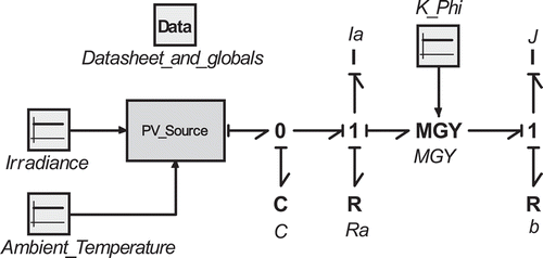
The model presented in this paper has an advantage over other models. As it is based on Bond Graphs, it allows interfacing with models of converters or direct loads of different nature. This interconnection is not possible in other models, which focus on making an annual power production estimated and economic factors associated with the possible installation of a photovoltaic plant. The interconnection capacity of the proposed model can facilitate the study of techniques for monitoring and track the maximum power point, as well as improvements in converters. There are numerous possibilities of subsystems that can be interconnected with the proposed photovoltaic source model. To illustrate this feature, consider the system modelled in Figure 15, in which the Kyocera KD33GX-LFE module is connected to a direct current machine.

Figure 15. Model involving a KD33GX-LFE PV module and a D-C machine.

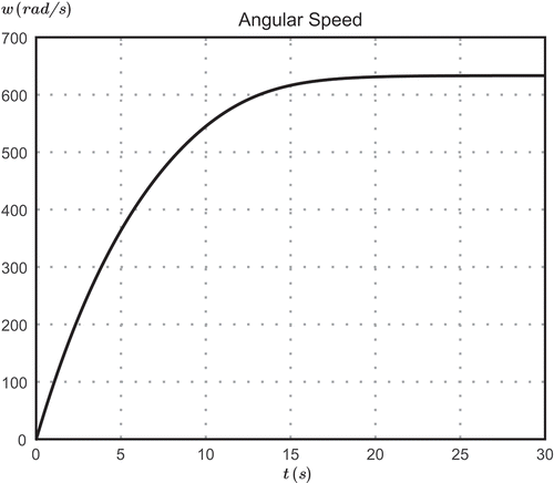
The model in Figure 15 is just a simple example of the interconnection capacity of the proposed model. Only for illustrative purposes, Figure 16 shows the angular velocity response of the DC motor.

Figure 16. Angular speed response of the D-C motor.

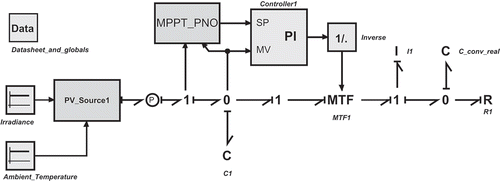
A final test showing the interconnectivity capability of the proposed model consists of the simulation of an MPPT controller connected to a buck converter, according to the model of Figure 17.

Figure 17. Proposed model interconnected with an MPPT controller.

In the model of Figure 17, the control scheme consists of disturbing the reference voltage according to the known perturb and observe method [32]. This control strategy is somewhat independent of Bond Graph modelling, and 20sim allows its proper construction. The model of the buck converter is based on the average model with transformer presented in [33].

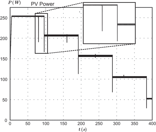
The simulation scenario is formed according to the following: The load resistance R starts with a value of 0.2 ohms and every 80 s it suddenly increases its value by 0.625 ohms. The irradiance begins with a value of 1000 and every 96 s decreases its value by 200. Figure 18 shows the power curve at the output of the photovoltaic array. The control algorithm is of the climbing the hill type. Right tracking to sudden changes in both the load and the source (irradiance) is made. Therefore, an adequate behaviour of the proposed model can be observed.

Figure 18. Power in the PV module under the control of the MPPT.

Concerning the computational cost required by the photovoltaic source model presented in this paper, all simulations were performed using Runge–Kutta methods. It is known that in these methods the main computational effort is required in evaluating the functions that form the state equations [34]. Additionally, at each integration step, the proposed model should perform the calculation of the parameters described by the equations shown in Figure 6. However, these equations are algebraic, and therefore do not add too much computational cost. Particularly, the model in Figure 15 contains three state variables, therefore the Runge–Kutta fourth-order method involves $12$ function evaluations at each integration step. The plot of Figure 16 is obtained from a simulation made in a time span from 0 to 30 s. An integration step of 0.01 s has been chosen. Therefore 3000 points are obtained. This simulation runs in 0.16 s on a computer with Pentium dual-core 2.5 GHz processor.

4. Conclusions

The experimental behaviour of the proposed model has been satisfactory, as it allowed to approximate with sufficient precision the actual $V-P$ curves of photovoltaic modules. Also, the proposed model required only information contained in the manufacturer’s data sheet, which makes it a very affordable option for a preliminary estimate of operation before any expenditure. In contrast, other models present in the literature can show excellent accuracy, but with the disadvantage of requiring large amounts of experimental data obtained by additional tests.

The used 4-parameter approach provided simplicity in the numerical solution of the non-linear implicit equations, allowing short simulation times. The 4th order Runge–Kutta method was sufficient to carry out the simulations presented in the paper. Comparatively, other models require the solution of more complicated implicit systems, which involves the disadvantage of forced use of more robust numerical methods and the inherent higher computational cost. Besides, not a significative difference between the 5-parameter and 4-parameter models was observed.

Being based on Bond Graph modelling, the proposed model presents an extensive interconnection capacity, which makes it a suitable tool for the study of the problems associated with the equipment connected to a photovoltaic array. The DC machine example shown in the paper was chosen for its simplicity, and a more elaborate example concerning an MPPT controller has been presented. Meanwhile, most of the existing models focus on predicting power generation, or in the study of economic aspects, showing no interconnection capacity with other associated physical systems. The presented model can also be adequately implemented in Modelica, due to the similarities that such modelling language shares with the Bond Graphs.

Another feature that was successful was the ability of the model to reproduce the phenomenon of partial shading. This feature is not standard on most existing models which consider only the incidence of uniform irradiance. The results show that the proposed model facilitates the study of the problems associated with partial shadings, such as the tracking of global maximum power point. It was possible to observe the simulation of the proposed model as a source for a converter with MPPT control. In this way, testing the converter can be made at simulation level, allowing the study of control algorithms before their physical implementation. Another line of future research is the simulation of hybrid generation systems comprising PV modules along with other forms of generation, both traditional and alternative. The model also allows studying problems related to power quality in PV arrays interconnected with the power grid.

Appendix.

Notation

Table

$a$	Five-parameter model modified ideality factor
$D_{in}$	Input data set
$D_{in,STC}$	Input data set under STC
$G$	Irradiance
$G_{STC}$	Irradiance under STC
$I$	PV current
$I_0$	Reverse saturation current
$I_D$	Diode current
$I_{MP}$	Maximum power current
$I_{MP,STC}$	Maximum power current under STC
$I_{ph}$	Photocurrent
$I_{SC}$	Short circuit current
$I_{SC,STC}$	Short circuit current under STC
$k$	Boltzmann constant
$n$	Ideality factor
$n_s$	Number of series cells in an array
$n_{se}$	Number of series cells in a section
$NOCT$	Nominal operating cell temperature
$P_{MP}$	Maximum power
$P_{MP,STC}$	Maximum power under STC
$q$	Electron charge
$R_p$	Parallel resistance
$R_s$	Series resistance
$T_a$	Ambient temperature
$T_C$	PV temperature
$T_{C,STC}$	PV temperature under STC
$V$	PV voltage
$V_D$	Diode voltage
$V_{MP}$	Maximum power voltage
$V_{MP,STC}$	Maximum power voltage under STC
$V_{OC}$	Open circuit voltage
$V_{OC,STC}$	Open circuit voltage under STC
${\alpha }_I$	Temperature coefficient of short circuit current
${\alpha }_P$	Temperature coefficient of power
${\alpha }_V$	Temperature coefficient of open circuit voltage
$\mathrm{\Lambda }$	4-parameter model exponential factor

References

- H. Wirth, Recent Facts about Photovoltaics in Germany, Institute for Solar Energy Systems Fraunhofer ISE, 2018.
- P.P. Altermatt, Models for numerical device simulations of crystalline silicon solar cells—a review, J. Comput. Electron. 10 (1 Sep 2011), p. 314. doi:10.1007/s10825-011-0367-6
- S.K. Firth, K.J. Lomas, and S.J. Rees, A simple model of PV system performance and its use in fault detection, Solar Energy 84 (30 Apr 2010), pp. 624–635. doi:10.1016/j.solener.2009.08.004
- D.L. Evans, Simplified method for predicting photovoltaic array output, Solar energy 27 (6) (1981), pp. 555–560. doi:10.1016/0038-092X(81)90051-7
- G.T. Klise and J.S. Stein, Models Used to Assess the Performance of Photovoltaic Systems, Freiburg: Sandia National Laboratories; 2009.
- D.L. King, W.E. Boyson, and J.A. Kratochvill, Photovoltaic Array Performance Model, U.S.A: Sandia National Laboratories; 2004.
- V.J. Chin, Z. Salam, and K. Ishaque, Cell modelling and model parameters estimation techniques for photovoltaic simulator application: a review, Appl. Energy. 15 (154) (Sep 2015), pp. 500–519. doi:10.1016/j.apenergy.2015.05.035
- K. Ishaque, Z. Salam, H. Taheri, and A. Shamsudin, A critical evaluation of EA computational methods for photovoltaic cell parameter extraction based on two diode model, Solar Energy 85 (30 Sep 2011), pp. 1768–1779. doi:10.1016/j.solener.2011.04.015
- W. De Soto, S.A. Klein, and W.A. Beckman, Improvement and validation of a model for photovoltaic array performance, Solar Energy 80 (1) (2006), pp. 78–88. doi:10.1016/j.solener.2005.06.010
- T.U. Townsend, A method for estimating the long term performance of direct coupled photovoltaic systems, M.S. Thesis, University of Wisconsin- Madison, 1989.
- W. Borutzky, Bond Graph Methodology: Development and Analysis of Multidisciplinary Dynamic System Models, Springer-Verlag, London, 2010.
- T.A. Pedersen and E. Pedersen, Bond graph modelling of marine power systems, Math. Comput. Model. Dyn. Syst. 18 (1 Apr 2012), pp. 153–173. doi:10.1080/13873954.2011.603735
- D.C. Karnopp, D.L. Margolis, and R.C. Rosenberg, System Dynamics: Modeling and Simulation of Mechatronic Systems, 4th ed., John Wiley and Sons, Hoboken, NJ, 2006.
- A. Woyte, J. Nijs, and R. Belmasn, Partial shadowing of photovoltaic arrays with different system configurations: literature review and field test results, Solar Energy 74 (3) (2003), pp. 217–233. doi:10.1016/S0038-092X(03)00155-5
- M.C. Alonso-Garca, J.M. Ruiz, and F. Chenlo, Experimental study of mismatch and shading effects in the I–V characteristic of a photovoltaic module, Solar Energy Mater. Solar Cells 90 (3) (2006), pp. 329–340. doi:10.1016/j.solmat.2005.04.022
- J. Young-Hyok, J. Doo-Yong, K. Jun-Gu, et al., A real maximum power point tracking method for mismatching compensation in PV array under partially shaded conditions, IEEE Trans. Power Electr. 26 (4) (2011), pp. 1001–1009. doi:10.1109/TPEL.2010.2089537
- D. Kun, B. XinGao, L. HaiHao, et al., A MATLAB-simulink-based PV module model and its application under conditions of nonuniform irradiance, IEEE Trans. Energy Convers. 27 (4) (2012), pp. 864–872. doi:10.1109/TEC.2012.2216529
- A.H. Rahim and M.T. Hussain, Evaluation and enhancement of dynamic performance of a microgrid including PV and wind generation systems, Math. Comput. Model. Dyn. Syst. 19 (1 Jun 2013), pp. 201–219. doi:10.1080/13873954.2012.719526
- H.M. Paynter, Analysis and Design of Engineering Systems, Cambridge, MA: MIT press; 1961.
- M. Wolf and H. Rauschenbach, Series resistance effects on solar cell measurements, Adv. Energy Convers. 3 (2) (1963), pp. 455–479. doi:10.1016/0365-1789(63)90063-8
- J.A. Gow and C.D. Manning, Development of a photovoltaic array model for use in power-electronics simulation studies, IEE Proc. Electric. Power Appl. 146 (2) (1999), pp. 193–200.
- W. Shockley, The theory of p-n junctions in semiconductors and p-n junction transistors, Bell Syst. Tech. J. 28 (3) (1949), pp. 435–489. doi:10.1002/j.1538-7305.1949.tb03645.x
- U. Eicker, Solar Technologies for Buildings, John Wiley and Sons, Chichester, England, 2003.
- R.G. Ross, Design techniques for flat-plate photovoltaic arrays. Proceedings of the 15th IEEE Photovoltaic Specialists Conference, IEEE, Orlando, FL, 12–15 may 1981, pp. 811–817.
- D.P. Hohm and M.E. Roop, Comparative study of maximum power point tracking algorithms, Prog. Photovoltaics Res. Appl. 11 (1) (2003), pp. 47–62. doi:10.1002/pip.459
- B. Marion, Comparison of predictive models for PV module performance. Proceedings of the 33rd IEEE Photovoltaics Specialists Conference, IEEE, San Diego, CA, 11–16 may 2008, pp. 1–6.
- 20-sim [internet]. Controllab Products, Enschede, The Netherlands. [cited 2016 Jun 15th]. Available at http://www.20sim.com/
- P. Fritzson and P. Bunus, Modelica-a general object-oriented language for continuous and discrete-event system modeling and simulation. Proceedings of the 35th Annual Simulation Symposium, IEEE, 2002 Apr 14, pp. 365–380.
- V. Leite and F. Chenlo, An improved electronic circuit for tracing the I-V characteristics of photovoltaic modules and strings. Proceedings of the International Conference on Renewable Energies and Power Quality, Granada, Spain, 23–25 Mar 2010.
- Humusoft [internet]. Humusoft S. R. O,, Prague, Czech Republic. [cited 2016 Jun 15th]. Available at http://www.humusoft.com/
- MATLAB [Internet]. MathWorks, Natick, MA. [cited 2016 Jun 15]. Available at http://www.mathworks.com/
- M.A. Eltawil and Z. Zhao, MPPT techniques for photovoltaic applications, Renewable Sustainable Energy Rev. 30 (25) (Sep 2013), pp. 793–813. doi:10.1016/j.rser.2013.05.022
- B. Allard, H. Helali, C.C. Lin, and H. Morel, Power converter average model computation using the bond graph and petri net techniques. Power Electronics Specialists Conference, 1995. PESC’95 Record., 26th Annual IEEE, Vol. 2, IEEE, San Diego, CA, 1995 Jun 18, pp. 830–836.
- R.L. Burden and J.D. Faires, Numerical Analysis, 9th ed., Cengage Learning, Brooks/Cole, Boston MA, 2011.