Empirical Gramian-based spatial basis functions for model reduction of nonlinear distributed parameter systems

ABSTRACT

Correct selection of spatial basis functions is crucial for model reduction for nonlinear distributed parameter systems in engineering applications. To construct appropriate reduced models, modelling accuracy and computational costs must be balanced. In this paper, empirical Gramian-based spatial basis functions were proposed for model reduction of nonlinear distributed parameter systems. Empirical Gramians can be computed by generalizing linear Gramians onto nonlinear systems, which results in calculations that only require standard matrix operations. Associated model reduction is described under the framework of Galerkin projection. In this study, two numerical examples were used to evaluate the efficacy of the proposed approach. Lower-order reduced models were achieved with the required modelling accuracy compared to linear Gramian-based combined spatial basis function- and spectral eigenfunction-based methods.

KEYWORDS:

• Distributed parameter systems
• model reduction
• spatial basis functions
• empirical balanced truncation

1. Introduction

In recent years, control of the microstructure, fluid flow, spatial profile and product size distribution of materials in advanced technologies has attracted much attention. These physical, chemical and biological processes lead to nonlinear distributed parameter systems (DPSs). In these systems, the spatial variable is distributed continuously in the target domain. The inputs and outputs depend on this parameter and can vary both temporally and spatially. For this reason, the dimensions of the reduced model are important for control design and simulations of nonlinear DPSs. Recently, several special journal issues organized by Munusamy et al. [1], Pourkargar and Armaou [2,3], Rad et al. [4], Ren et al. [5,6], Zheng et al. [7], Qi et al. [8,9], Izadi and Dubljevic [10], Lu et al. [11–13] and Christofides [14–16] have focused on this topic. To obtain reduced models satisfactory for use in engineering applications and that balance modelling accuracy and computational cost, the correct spatial basis functions under the framework of time–space separation must be selected. Several popular spatial basis functions, including Fourier series [17], orthogonal polynomials [18] and eigenfunctions of distributed parameter processes [19,20], have been introduced. However, these spatial basis functions are general and result in relatively low modelling accuracy. As a result, reduced models using these basis functions must include high-order expansions for a given accuracy, rendering it difficult to implement controller design for nonlinear DPSs.

In the spectral method, empirical eigenfunctions (EEFs) previously identified by Karhunen–Loève (KL) decomposition [21] are often used as spatial basis functions [10,22–26]. EEFs provide a spatial structure for a given dimension that captures the largest fraction of kinetic energy and can be easily calculated from eigenvalue problem solutions. However, in engineering applications, obtaining EEFs from representative process data is dependent on the locations and number of sensors. In these applications, only input–output data are available, which can only be used to obtain a limited number of EEFs due to the placement of a limited number of sensors and actuators in the target system. This will decrease the prediction accuracy of the reduced model. Conversely, KL decomposition is a method of linear model reduction that can only produce a linear approximation for the original nonlinear problem. Although it has good computational efficiency, KL decomposition should be implemented carefully when modelling and analysing engineering problems [17,27–30].

Recently, transformation methods have been proposed for deriving a new set of spatial basis functions for model reduction of nonlinear DPSs [17,27,31] and created using the vector of general basis functions to multiply by a transformation matrix, which is computed by numerical optimization [20,27,31] or the balanced truncation method [32,33]. The former was first introduced by Kwasniok [17,27] and accounts for the dynamics of the reduced model by defining basic spatial patterns, called principal interaction patterns, and then developing an optimization algorithm for reducing the high-dimensional Fourier–Galerkin approximation to a low-dimensional system. However, variational principle for principal interaction patterns in this algorithm requires high-dimensional nonlinear minimization. Jiang and Deng [31] proposed a similar method that is implemented using numerical optimization for a spatially and temporally integrated squared error function related to the transformation matrix and a high-dimensional nonlinear minimization with numerous parameters. Application of these numerical optimization methods in calculating transformation matrices is limited by computational efficiency.

With lower computational costs than other optimization methods, the balanced truncation method [32] is used to calculate transformation matrices to derive linear Gramians-based combined spatial basis functions. This method has higher modelling accuracy than the spectral method and has been successfully applied in modelling of thermal crown in hot rolling processes [33]. However, this linear Gramians-based method can only be applied in linear ordinary differential equation (ODE) systems, which approximate the nonlinear temporal dynamics of DPSs by simply ignoring the existing nonlinear terms. This method may be effective for some nonlinear DPSs [32,33] but is ineffective or unsatisfactory for others. For processes with strongly nonlinear dynamics, the linear ODE system will have difficulties obtaining a good approximation for nonlinear problems. Instead, empirical Gramians [34,35], which are calculated by taking into explicit account the input–output behaviours of the systems, are proposed for model reduction of these nonlinear systems. These Gramians generalize the methods from linear model reduction theory, and the computational requirements are the solutions of the standard matrix eigenvalue problems. Therefore, linear Gramians-based combined spatial basis functions can be improved because of uncertain modelling accuracy.

In this paper, empirical Gramians-based combined spatial basis functions are proposed for model reduction of nonlinear DPSs. Empirical Gramians can be calculated directly from the nonlinear temporal dynamics of DPSs at any operating point and are balanced to obtain the matrices of combination coefficients for spatial basis functions. Because empirical Gramians are computed by generalizing Gramians from linear systems to nonlinear systems, the proposed method provides a model reduction framework for nonlinear DPSs. For a given modelling accuracy requirement, lower dimensions of the reduced models can be achieved with this method compared to other methods using linear Gramians-based combined spatial basis functions. Two numerical examples are used to demonstrate the efficacy of the proposed method. This paper is organized as follows: The spectral-based modelling approaches are discussed in Section 2. Empirical Gramians-based combined spatial basis functions are introduced in Section 3. Numerical examples and results are provided in Section 4. Concluding remarks are made in Section 5.

2. Spectral-based modelling

Typical examples of nonlinear DPSs include thermal, fluid and convection–diffusion–reaction processes, which can be governed by partial differential equations (PDEs) with the following state description:

(1) $\begin{array}{rl}& \frac{\mathrm{\partial }X\left(z,t\right)}{\mathrm{\partial }t}=\mathcal{A}X\left(z,t\right)+\mathcal{B}U\left(z,t\right)+F\left(X,\frac{\mathrm{\partial }X}{\mathrm{\partial }z},\cdots ,U,\frac{\mathrm{\partial }U}{\mathrm{\partial }z},\cdots \right),\\ & Y\left(z,t\right)=\mathcal{C}X\left(z,t\right),\end{array}$(1)

where $t\in [0,\mathrm{\infty })$ is the time variable. Equation (1) is considered a bounded spatial domain $\mathrm{\Omega }$ and is subject to a number of boundaries and initial conditions. In Equation (1), spatial variable $z$ is a parameter distributed continuously throughout target domain $\mathrm{\Omega }$, where only one spatial dimension is considered. The state variable $X\left(z,t\right)$ and manipulated input $U\left(z,t\right)$ depend on parameter $z$ and time variable $t$, respectively, where $U(z,t)={\sum }_{i=1}^p{u}_i(t)h_i(z)$ denotes the spatio-temporal input with $p$ temporal inputs $u_i(t)$ and spatial distributions $h_i(z)$. $\mathcal{A}$ and $\mathcal{B}$ are linear operators involving linear spatial derivatives for $X\left(z,t\right)$ and $U\left(z,t\right)$. The measured output of the DPS (1) is $Y\left(z,t\right)$ and $\mathcal{C}$ is the corresponding linear operator of the state variable $X\left(z,t\right)$. $F(X,\mathrm{\partial }X/\mathrm{\partial }z,\cdots ,U,\mathrm{\partial }U/\mathrm{\partial }z,\cdots )$ denotes a nonlinear function of $X\left(z,t\right)$ and $U\left(z,t\right)$ and their spatial derivatives. The phase space of Equation (1) is assumed from the infinite-dimensional Hilbert space $H(\mathrm{\Omega })$ of sufficiently smooth functions from $\mathrm{\Omega }$ into real numbers. A scalar product introduced in $H(\mathrm{\Omega })$ is obtained from

(2) $\left[g\left(z\right),h\left(z\right)\right]={\int }_{\mathrm{\Omega }}g\left(z\right)h\left(z\right)dz$(2)

for arbitrary functions $g(z),h(z)\in H(\mathrm{\Omega })$.

Model reduction of PDEs is mainly performed using spatial basis function expansions and the Galerkin method. This paper focuses on PDEs that can be partitioned into slow and fast modes [19,20]. Assuming the remaining modes contribute little to the whole system, only the first $N$ modes in the expansions will be retained in practice. In some situations, $N$ may have a very large value [20,33]. The Galerkin projection of Equation (1) for the preselected spatial basis function $\left\{{\phi }_1(z),{\phi }_2(z),\cdots ,{\phi }_N(z)\right\}$ results in a dynamical system for the corresponding time evolution $x(t)=[x_1(t),x_2(t),\cdots x_N(t){]}^T$:

(3) $\begin{array}{c}\dot{x}\left(t\right)=Ax\left(t\right)+Bu\left(t\right)+f\left(x\left(t\right),u\left(t\right)\right),\\ y\left(t\right)=Cx\left(t\right),\end{array}$(3)

where $y(t)=[Y(z_1,t),Y(z_2,t),\cdots ,Y(z_L,t){]}^T$ and $\left\{Y(z_i,t),i=1,\cdots ,L\right\}$ denote the measured output at $L$ spatial locations $z_1,z_2,\cdots ,z_L$. $u(t)=[u_1(t),u_2(t),\cdots ,u_p(t){]}^T$ is the vector of the temporal inputs. $A_{N\times N}$, $B_{N\times p}$, and $C_{L\times N}$ are constant matrices and $f(x(t),u(t))$ is the nonlinear function of $x(t)$ and $u(t)$.

3. Empirical Gramians-based combined spatial basis functions

3.1 Computation of combined coefficients

Combined basis functions are linear combinations of preselected spatial basis functions, where the combination coefficients are calculated according to the temporal dynamics of the system. There are two methods of computing the matrix of combination coefficients: balanced truncation and balancing of empirical Gramians [34]. Empirical Gramians generalize linear Gramians for use in nonlinear systems and can be balanced using the same balanced truncation method used for linear systems. When applied to linear systems, this results in linear Gramians [34]. Before proceeding further, we will provide preliminary definitions based on theories developed for linear systems.

3.1.1 Balanced truncation method

Neglecting the nonlinear terms of Equation (3), a linear time-invariant system can be obtained as follows:

(4) $\begin{array}{c}\dot{x}\left(t\right)=Ax\left(t\right)+Bu\left(t\right),\\ y\left(t\right)=Cx\left(t\right).\end{array}$(4)

If the linear time-invariant system (4) is open-loop stable, a controllability Gramian, $W_{C,\mathrm{l}\mathrm{i}\mathrm{n}}$, and an observability Gramian, $W_{O,\mathrm{l}\mathrm{i}\mathrm{n}}$ [34,35], can be computed from:

(5) $W_{C,\mathrm{l}\mathrm{i}\mathrm{n}}={\int }_0^{\mathrm{\infty }}{\mathrm{e}}^{At}B{B}^T{\mathrm{e}}^{A^{T}t}dt,$(5)

(6) $W_{O,\mathrm{l}\mathrm{i}\mathrm{n}}={\int }_0^{\mathrm{\infty }}{\mathrm{e}}^{A^{T}t}{C}^{T}C{\mathrm{e}}^{At}dt.$(6)

If the system is stable and controllable, the controllability Gramian (5) will have full rank. Similarly, the observability Gramian (6) will have full rank for stable and observable systems. Furthermore, the linear Gramians $W_{C,\mathrm{l}\mathrm{i}\mathrm{n}}$ and $W_{O,\mathrm{l}\mathrm{i}\mathrm{n}}$ are the unique positive definite solutions of the Lyapunov equations $A{W}_{C.\mathrm{l}\mathrm{i}\mathrm{n}}+W_{C,\mathrm{l}\mathrm{i}\mathrm{n}}{A}^T=-B{B}^T$ and $A^T{W}_{O,\mathrm{l}\mathrm{i}\mathrm{n}}+W_{O,\mathrm{l}\mathrm{i}\mathrm{n}}A=-C^{T}C$ respectively.

The balanced form of the linear system (4) transforms the controllability Gramian $W_{C,\mathrm{l}\mathrm{i}\mathrm{n}}$ and observability Gramian $W_{O,\mathrm{l}\mathrm{i}\mathrm{n}}$ into being equal as follows:

(7) ${\hat{W}}_{C,\mathrm{l}\mathrm{i}\mathrm{n}}={\hat{W}}_{O,\mathrm{l}\mathrm{i}\mathrm{n}}=\mathrm{d}\mathrm{i}\mathrm{a}\mathrm{g}\left({\sigma }_1,{\sigma }_2,\cdots ,{\sigma }_N\right),$(7)

where ${\sigma }_1\ge {\sigma }_2\ge {\sigma }_3\ge \cdots {\sigma }_N\ge 0$ and ${\sigma }_i$ denote the $i$th Hankel singular value [35]. For the controllability Gramian, the Hankel singular values correspond to the amount of energy that has to be put into the system in order to move the corresponding states. The singular values of the observability Gramians refer to the energy generated by the corresponding states. If the linear system (4) is balanced, the state with the largest singular value is the one most affected by control moves and the output is the most affected by a change in this state. Therefore, the states corresponding to the largest singular values influence the input–output behaviours the most. The transformed Gramians are then obtained from:

(8) ${\hat{W}}_{C,\mathrm{l}\mathrm{i}\mathrm{n}}=S_b{W}_{C,\mathrm{l}\mathrm{i}\mathrm{n}}{S}_b^T,{\hat{W}}_{O,\mathrm{l}\mathrm{i}\mathrm{n}}={\left({S_b}^{-1}\right)}^T{W}_{O,\mathrm{l}\mathrm{i}\mathrm{n}}{S_b}^{-1},$(8)

where $S_b$ denotes the transformation matrix.

Moore [36] introduced balancing as a tool for model reduction. If a linear system is balanced, Hankel singular values provide a measure for the importance of the states. For model reduction, states that contribute very little to the input–output behaviours can be eliminated and the reduced system can serve as a suboptimal approximation of the full-order system. In previous work [32], the first $k$ columns of the balanced matrix $S_b$ were set as a $N\times k$ matrix and the elements were the combination coefficients from the preselected spatial basis functions.

3.1.2 Balancing of empirical Gramians

Balancing of linear systems is a powerful and simple technique. However, general nonlinear balancing cannot be efficiently implemented [37]. Balancing of empirical Gramians combines the easy-to-use linear approaches with the flexibility required for nonlinear systems. In many studies [34,35], empirical Gramians have been proposed for analysis and model reduction of nonlinear systems in a prespecified operating region. The data for constructing empirical Gramians may be obtained from either simulations or experiments. The procedure used for balancing linear systems can also be used to balance empirical Gramians.

The proposed approach calculates the empirical Gramians from the nonlinear ODE system process data (3). $T^p=\left\{T_1,T_2,\cdots ,T_{r_1}\right\}$ is a set of $r_1$ orthogonal $p\times p$ matrices, where $r_1$ denotes the number of matrices for the excitation/perturbation directions. $M^{s_1}=\left\{c_1,c_2,\cdots ,c_{s_1}\right\}$ is a set of $s_1$ positive constants, where $s_1$ denotes the number of different excitation/perturbation sizes for each direction. $E^p=\left\{e_1,e_2,\cdots ,e_p\right\}$ is the $p$ standard unit vector in ${\mathcal{R}}^p$, where $p$ denotes the number of inputs in the system (3). Given the temporal function $x(t)$, the mean $\bar{x}(t)$ is defined using $\bar{x}(t)=\underset{T_{max}\to \mathrm{\infty }}{lim}\frac{1}{T_{max}}{\int }_0^{T_{max}}x(t)dt$. The empirical controllability Gramian of the nonlinear system (3) can be defined as:

(9) $W_{C,\mathrm{n}\mathrm{o}\mathrm{n}\mathrm{l}\mathrm{i}\mathrm{n}}=\sum _{l=1}^{r_1}\sum _{m=1}^{s_1}\sum _{i=1}^p\frac{1}{r_1{s}_1{c}_m^2}\underset{0}{\overset{\mathrm{\infty }}{\int }}{\mathrm{\Phi }}^{\mathrm{i}\mathrm{l}\mathrm{m}}\left(t\right)dt,$(9)

where ${\mathrm{\Phi }}^{\mathrm{i}\mathrm{l}\mathrm{m}}(t)\in {\mathrm{\Re }}^{N\times N}$ is obtained from

(10) ${\mathrm{\Phi }}^{\mathrm{i}\mathrm{l}\mathrm{m}}\left(t\right)=\left(x^{\mathrm{i}\mathrm{l}\mathrm{m}}\left(t\right)-{\bar{x}}^{\mathrm{i}\mathrm{l}\mathrm{m}}\right){\left(x^{\mathrm{i}\mathrm{l}\mathrm{m}}\left(t\right)-{\bar{x}}^{\mathrm{i}\mathrm{l}\mathrm{m}}\right)}^T$(10)

In Equation (10), $x^{\mathrm{i}\mathrm{l}\mathrm{m}}(t)$ is the state of the system (3) corresponding to the impulsive input $u(t)=c_m{T}_l{e}_i\delta (t)$ and ${\bar{x}}^{\mathrm{i}\mathrm{l}\mathrm{m}}$ denotes the mean state of $x^{\mathrm{i}\mathrm{l}\mathrm{m}}(t)$. The empirical controllability Gramian is a computable generalization of the controllability Gramian onto nonlinear systems. Lall et al. [34] demonstrated the empirical controllability Gramian of stable linear systems is equal to the usual controllability Gramian, where the eigenvectors of the empirical controllability Gramian corresponding to non-zero eigenvalues span a subspace containing a set of reachable states using the chosen initial impulsive inputs.

$T^N=\left\{T_1,T_2,\cdots ,T_{r_2}\right\}$ is a set of $r_2$ orthogonal $N\times N$ matrices, where $r_2$ denotes the number of matrices for the excitation/perturbation directions. $M^{s_2}=\left\{c_1,c_2,\cdots ,c_{s_2}\right\}$ is a set of $s_2$ positive constants, where $s_2$ denotes the number of different excitation/perturbation sizes for each direction. $E^N=\left\{e_1,e_2,\cdots ,e_N\right\}$ is $N$ standard unit vectors in ${\mathcal{R}}^N$. The empirical observability Gramian of the nonlinear system (3) can be defined as:

(11) $W_{O,\mathrm{n}\mathrm{o}\mathrm{n}\mathrm{l}\mathrm{i}\mathrm{n}}=\sum _{k=1}^{r_2}\sum _{n=1}^{s_2}\frac{1}{r_2{s}_2{c}_n^2}\underset{0}{\overset{\mathrm{\infty }}{\int }}{T}_k{\mathrm{\Psi }}^{kn}\left(t\right)T_k^{T}dt,$(11)

where ${\mathrm{\Psi }}^{kn}(t)\in {\mathrm{\Re }}^{N\times N}$ is obtained using

(12) ${\mathrm{\Psi }}_{ij}^{kn}\left(t\right)={\left(y^{ikn}\left(t\right)-{\bar{y}}^{ikn}\right)}^T\left(y^{jkn}\left(t\right)-{\bar{y}}^{jkn}\right)$(12)

In Equation (12), $y^{ikn}(t)$ is the output of the nonlinear system (3) corresponding to the initial condition $x_0=c_n{T}_k{e}_i$, where $u(t)=0$ and ${\bar{y}}^{ikn}$ denote the mean state of $y^{ikn}(t)$.

The empirical observability Gramian is a computable generalization of the usual observability Gramian for nonlinear systems. Lall et al. [34] demonstrated that the empirical observability Gramian of stable linear systems is equal to the usual observability Gramian. Empirical controllability Gramians can be interpreted as the sum of the empirical Gramians of the states over time and for different combinations of input variables. Meanwhile, the empirical observability Gramians can be viewed as the sum of the covariance matrices of the outputs corresponding to different initial conditions. Rather than searching for exact controllability and observability submanifolds within the state space, the aim is to find subspaces that approximate these manifolds. Empirical Gramians provide a quantitative method for deciding upon the importance of particular subspaces of the state space with respect to the inputs and outputs of the system. Because empirical Gramians are by nature based upon discretely measured system properties, such as states and outputs, it is advantageous to reformulate them into a discrete form for numerical approximations [34,35]. This leads to balancing of empirical Gramians motivated by a standard idea from linear theories. A simple numerical technique [38] of balancing the (empirical) Gramians $W_{C,\mathrm{n}\mathrm{o}\mathrm{n}\mathrm{l}\mathrm{i}\mathrm{n}}$ and $W_{O,\mathrm{n}\mathrm{o}\mathrm{n}\mathrm{l}\mathrm{i}\mathrm{n}}$ is as follows. First, the Cholesky factorization [39] is applied to $W_{O,\mathrm{n}\mathrm{o}\mathrm{n}\mathrm{l}\mathrm{i}\mathrm{n}}$ so that $W_{O,\mathrm{n}\mathrm{o}\mathrm{n}\mathrm{l}\mathrm{i}\mathrm{n}}=Z{Z}^T$, where $Z$ is a lower triangular with non-negative diagonal entries. $U{\mathrm{\Sigma }}^2{U}^T$ is the eigenvalue decomposition of $Z^T{W}_{C,\mathrm{n}\mathrm{o}\mathrm{n}\mathrm{l}\mathrm{i}\mathrm{n}}Z$ and $S_b={\mathrm{\Sigma }}^{1/2}{U}^T{Z}^{-1}$. Then,

(13) $S_b{W}_{O,\mathrm{n}\mathrm{o}\mathrm{n}\mathrm{l}\mathrm{i}\mathrm{n}}{S_b}^T=({S_b}^{-1}{)}^T{W}_{C,\mathrm{n}\mathrm{o}\mathrm{n}\mathrm{l}\mathrm{i}\mathrm{n}}{S_b}^{-1}=\mathrm{\Sigma }.$(13)

To derive the combined spatial basis functions, the first $k$ columns of matrix $S_b$ are set as a $N\times k$ matrix of combined coefficients. Using the MATLAB style colon notation, the matrix is set as $\hat{S}=S_b(:,1:k)$.

3.2 Combined spatial basis functions for model reduction

Combined spatial basis functions are derived from linear combinations of the selected general basis functions:

(14) ${\varphi }_i\left(z\right)=\sum _{j=1}^N{\hat{S}}_{ji}{\phi }_j\left(z\right),i=1,2,\cdots ,k,$(14)

where the coefficient ${\hat{S}}_{ji}$ is the element in matrix $\hat{S}$ on the$j$th row and $i$th column. Then, Equation (14) can be rewritten as:

(15) $\mathrm{\Delta }\left(z\right)=\mathrm{\Lambda }\left(z\right)\cdot {\hat{S}}_{N\times k},$(15)

where $k<N$ and $\mathrm{\Delta }\left(z\right)=[{\varphi }_1(z),{\varphi }_2(z),\cdots ,{\varphi }_k(z)]$ and $\mathrm{\Lambda }\left(z\right)=[{\phi }_1(z),{\phi }_2(z),\cdots ,{\phi }_N(z)]$ denote the set of combined and general basis functions of Equation (1), respectively. The number of combined basis functions, $k$, is smaller than $N$, indicating that the corresponding reduced PDE model (1) will have smaller dimensions than Equation (3).

The real solution of the nonlinear PDE (1) can be approximated using the following expansions of the combined basis functions (15) with corresponding temporal coefficients:

(16) $X_k\left(z,t\right)=\mathrm{\Delta }\left(z\right)\cdot \hat{x}\left(t\right),$(16)

where $\hat{x}(t)={\left[{\hat{x}}_1(t),{\hat{x}}_2(t),\cdots ,{\hat{x}}_k(t)\right]}^T$ denotes the vector of the temporal variable. The equation residual of the PDE (1) using the expansion (16) is as follows:

(17) $R_k\left(z,t\right)=\left(\frac{\mathrm{\partial }{X}_k}{\mathrm{\partial }t}\right)-\left(\mathcal{A}{X}_k+\mathcal{B}U+F\left(X_k,\frac{\mathrm{\partial }{X}_k}{\mathrm{\partial }z},\cdots ,U,\frac{\mathrm{\partial }U}{\mathrm{\partial }z},\cdots \right)\right),$(17)

which is minimized within spatial domain $\mathrm{\Omega }$ using:

(18) ${\int }_{\mathrm{\Omega }}{R}_k\left(z,t\right){\phi }_i\left(z\right)dz=0.$(18)

Substituting Equations (15), (16) and (17) into Equation (18), the following is derived:

(19) $\begin{array}{rl}& \frac{\mathrm{\partial }\left(\mathrm{\Lambda }\left(z\right)\hat{S}\hat{x}\left(t\right)\right)}{\mathrm{\partial }t}=\mathcal{A}\left(\mathrm{\Lambda }\left(z\right)\hat{S}\hat{x}\left(t\right)\right)+\mathcal{B}\left({\sum }_{i=1}^p{u}_i(t)h_i(z)\right)\\ & +F\left(\mathrm{\Lambda }\left(z\right)\hat{S}\hat{x}\left(t\right),\frac{\mathrm{\partial }\left(\mathrm{\Lambda }\left(z\right)\hat{S}\hat{x}\left(t\right)\right)}{\mathrm{\partial }z},\cdots ,\sum _{i=1}^p{u}_i(t)h_i(z),\frac{\mathrm{\partial }\left({\sum }_{i=1}^p{u}_i(t)h_i(z)\right)}{\mathrm{\partial }z},\cdots \right).\end{array}$(19)

Using the Galerkin method [40], the following equation is then obtained:

(20) $\begin{array}{rl}& {\int }_{\mathrm{\Omega }}\frac{\mathrm{\partial }\left(\mathrm{\Lambda }\left(z\right)\hat{S}\hat{x}\left(t\right)\right)}{\mathrm{\partial }t}{\phi }_i\left(z\right)dz={\int }_{\mathrm{\Omega }}\left(\mathcal{A}\left(\mathrm{\Lambda }\left(z\right)\hat{S}\hat{x}\left(t\right)\right)+\mathcal{B}\left({\sum }_{i=1}^p{u}_i(t)h_i(z)\right)\right){\phi }_i\left(z\right)dz\\ & +{\int }_{\mathrm{\Omega }}F\left(\mathrm{\Lambda }\left(z\right)\hat{S}\hat{x}\left(t\right),\frac{\mathrm{\partial }\left(\mathrm{\Lambda }\left(z\right)\hat{S}\hat{x}\left(t\right)\right)}{\mathrm{\partial }z},\cdots ,\right. \\ & \left. {\sum }_{i=1}^p{u}_i(t)h_i(z),\frac{\mathrm{\partial }\left({\sum }_{i=1}^p{u}_i(t)h_i(z)\right)}{\mathrm{\partial }z},\cdots \right){\phi }_i\left(z\right)dz,\end{array}$(20)

where $i=1,2,\cdots ,N$. Integrating Equation (20) and using the matrix computations, an ODE system with fewer modes is obtained using:

(21) $\begin{array}{rl}& \dot{\hat{x}}(t)={\hat{S}}^{\ast }A\hat{S}\hat{x}(t)+S^{\ast }Bu(t)+{\hat{S}}^{\ast }g(\hat{S}\hat{x}(t),u(t)),\\ & y(t)=C\hat{S}\hat{x}(t),\end{array}$(21)

where ${\hat{S}}^{\ast }$ denotes the generalized inverse matrix of $\hat{S}$, matrices $A,B,C$ are the same as in Equation (3) and $g(\hat{S}\hat{x}(t),u(t))$ is the nonlinear function of $\hat{x}(t)$ and $u(t)$. Equation (21) takes into explicit account the input–output connection and has similar input–output behaviours as the system (3).

Remarks: The combined spatial basis function-based model reduction described in this paper has similarities with the reduced basis methods described in Ref. [41]. The main goal of the reduced basis methods was to provide a reduced simulation scheme in which a function for a newly given parameter vector is determined as an approximation of the unknown detailed solution. The underlying reduced simulation scheme is based on a Galerkin projection of the detailed simulations onto a lower-dimensional space with rigorous a posteriori error bounds between the reduced and detailed solutions. This paper assumes the solution of a nonlinear PDE is expressed in a known set of spatial basis functions ${\left\{{\phi }_i\right\}}_{i=1}^N$ that span a high-dimensional space $\mathrm{\Gamma }$ for the spatial basis functions. The idea is to take advantage of available experimental data for the solution of the PDE to find subspace $\mathrm{\Theta }$ of $\mathrm{\Gamma }$. The subspace $\mathrm{\Theta }$ is spanned by a new basis, ${\left\{{\varphi }_i\right\}}_{i=1}^k$, where $k<N$, that is obtained from linear combinations of known basis ${\left\{{\phi }_i\right\}}_{i=1}^N$. Using the same number of spatial basis functions, the new basis-based modelling can better approximate the exact PDE solution (1) with lower computation costs.

However, the most important step for obtaining the new basis ${\left\{{\varphi }_i\right\}}_{i=1}^k$ is to calculate the matrix of combination coefficients according to the temporal dynamics. Balancing of empirical Gramians is employed to compute the balanced form for nonlinear ODE systems. The first $k$ columns of the transformation matrix are set as the matrix of combined coefficients. Because empirical Gramians are calculated by explicitly taking into account the input–output behaviours of nonlinear temporal systems, they provide a quantitative method of deciding upon the importance of particular subspaces of the state space. The temporal dynamics of the PDE are then considered when constructing the new basis ${\left\{{\varphi }_i\right\}}_{i=1}^k$ using the elements of the transformation matrix as the combined coefficients. Because the empirical Gramians include the controllability and observability Gramians of the stable linear system as a special case, the empirical Gramians-based balanced truncation preserves stability for the linearized model.

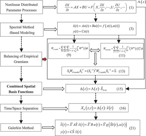
Summary: A model reduction framework using combined spatial basis functions for nonlinear DPSs is summarized in Figure 1.

Figure 1. The model reduction framework of the combined spatial basis functions.

4. Numerical examples

If the measured and predicted outputs of nonlinear DPSs are compared at $L$ spatial locations $z_1,z_2,\cdots ,z_L$ and sampling times $t_1,t_2,\cdots ,t_{\mathrm{N}\mathrm{t}\mathrm{i}\mathrm{m}}$, the root of mean square error (RMSE) between the dynamical process and approximation model as the performance index can be defined as follows:

(22) $\mathrm{R}\mathrm{M}\mathrm{S}\mathrm{E}=\sqrt{\frac{\sum _{i=1}^n\sum _{j=1}^{\mathrm{N}\mathrm{t}\mathrm{i}\mathrm{m}}{\left(Y\left(z_i,t_j\right)-\hat{Y}\left(z_i,t_j\right)\right)}^2}{L\cdot \mathrm{N}\mathrm{t}\mathrm{i}\mathrm{m}}},$(22)

where $Y(z_i,t_j)$ and $\hat{Y}(z_i,t_j)$ denote the measured and predicted outputs, respectively.

The numerical experiments were performed using a personal computer with an Intel(R) Pentium(R) CPU G620 @ 2.60GHz, RAM 4.00GB and Windows 7 operating system. MATLAB2009b was used to compute the numerical results, where the functions of the calculations used for balancing empirical Gramians from the data were provided by Hahn [42]. Routines for computing the empirical Gramians and balancing transformations are shown on this webpage along with several numerical examples of linear and nonlinear systems. In these MATLAB functions, the perturbation size of inputs, $c_m$, and the initial condition of the states are the input parameters needed to be set according to different numerical experiments.

The MATLAB function ode45, which is the (adaptive) embedded fourth–fifth-order Runge–Kutta method, was employed for integration of the ODE systems. The method used to compute the trajectories of the nonlinear ODE systems was similar to that described in Ref. [32]. Obtaining the exact analytical descriptions of nonlinear terms in Equation (21) based on time/space separation in new spatial basis functions was difficult because of the inner product of the combined spatial basis functions. Therefore, a feedforward BP neural network [43] was used to approximate these nonlinear terms, and the neural network tool in MATLAB toolboxes was employed to train the BP neural networks. According to the spectral-approximation-based intelligent modelling described in Ref. [20], a low-order hybrid model can be obtained to approximate DPS dynamics.

4.1. Catalytic rod

To evaluate model reduction by the proposed method, the spatio-temporal evolution of catalytic rod was studied [9,19,32]. Because this reaction is exothermic, a cooling medium is placed in contact with the rod. Assuming the rod has a constant density and heat capacity, constant conductivity and constant temperature at both sides and there is an excess of species in the furnace, the mathematical model describing the spatio-temporal evolution of the rod temperature consists of the following PDE:

(23) $\frac{\mathrm{\partial }X\left(z,t\right)}{\mathrm{\partial }t}=\frac{{\mathrm{\partial }}^{2}X\left(z,t\right)}{\mathrm{\partial }{z}^2}+{\beta }_T\left(e^{-\gamma /\left(1+X(z,t)\right)}-e^{-\gamma }\right)+{\beta }_u\left(h{\left(z\right)}^{T}u\left(t\right)-X\left(z,t\right)\right).$(23)

In this case, Equation (23) is subject to the following Dirichlet boundary and initial conditions:

(24) $X\left(0,t\right)=0,X\left(\pi ,t\right)=0,X\left(z,0\right)=X_0\left(z\right),$(24)

where $X(z,t),u(t),h(z),{\beta }_T,{\beta }_u$ and $\gamma$ denote the temperature in the reactor, manipulated input (temperature of the cooling medium), actuator distribution, heat of the reaction, heat transfer coefficient and activation energy, respectively. The process parameters are set as ${\beta }_T=50,{\beta }_u=2$ and $\gamma =4$. There are four actuators ($u(t)=[u_1(t),u_2(t),u_3(t),u_4(t){]}^T$) available with the spatial distribution functions $h(z)=[h_1(z),h_2(z),h_3(z),h_4(z){]}^T$ and $h_i(z)=H(z-(i-1)\pi /4)-H(z-i\pi /4),i=1,2,3,4$, and $H(\cdot )$ is the standard Heaviside function. The input signals are

(25) $u_i\left(t\right)=1.1+4sin(t/10+i/10),i=1,2,3,4.$(25)

The PDE solution from Equation (23) with the input from Equation (25) was computed for comparisons. Forty-one points were used for spatial discretization of the PDE, and the MATLAB function ode45 was utilized as the time integrator. Nineteen sensors used for measurements were supposed to be uniformly distributed in the space. The sampling interval $\mathrm{\Delta }t$ was 0.01 s and the simulation time was 4 s. The values of the state variable at every time sampling point for each sensor location were recorded and a set of data was collected from Equation (23). The initial condition $X_0(z)$ was set as $sin(z)$. First, a spectral-based model was developed where the basis functions family $\{\sqrt{2/\pi }sin(kz),k=1,2,\cdots ,\mathrm{\infty }\}$ was selected for time/space separation. According to the eigenspectrum of the spatial differential operator of Equation (23), a small ratio factor $\tau =\left(\left|Re\left({\lambda }_1\right)\right|\right)/\left(\left|Re\left({\lambda }_N\right)\right|\right)$ was generally used for the order determination, where ${\lambda }_1$ and ${\lambda }_N$ denote the corresponding eigenvalues of the first and $N$th spatial basis functions, respectively. If 0.1 (i.e. ${\lambda }_N$ is 10 times ${\lambda }_1$) is chosen, it will lead to a particular value for $N$ [20].

The balanced truncation method and balancing of empirical Gramians were employed to calculate the transformation matrices. In calculations of empirical Gramians, the perturbation size of the inputs was set to 0.1 and the initial condition of the states was set to be the steady state of the obtained finite-dimensional ODE system. Two types of spatial basis functions were then obtained through linear combinations. The approximation models can be derived based on two types of new basis functions and the RMSEs for the approximation of catalytic rod temperature calculated from the testing data, as shown in Figure 2.

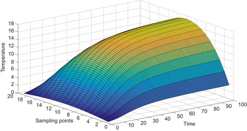
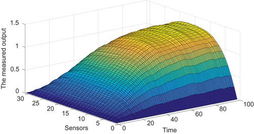
Figure 2. The measured time evolution of distributed temperature of catalytic rod for testing.

Figure 3 presents comparisons of the RMSEs from approximations based on general basis functions and the two new types of spatial basis functions, where one type consisted of new spatial basis functions derived from the balanced truncation method and the other type consisted of combined spatial basis functions derived by balancing empirical Gramians. As shown in Figure 3, the RMSEs of the approximation models based on the proposed method were much smaller than those from using general and new basis functions from the balanced truncation method. The small ratio factor was set to 0.1. Comparisons of eigenvalues revealed ${\lambda }_4$ was nearly 10 times ${\lambda }_1$. A spectral-based model with four modes was generally chosen to approximate the dominant dynamics of Equation (23).

Figure 3. The roots of mean square error based on spectral basis functions and two kinds of new spatial basis functions for spatio-temporal evolution of catalytic rod temperature.

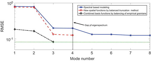
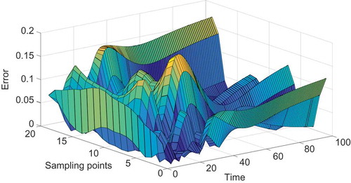
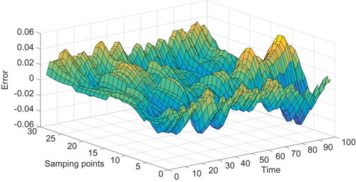
It is clear that the RMSE of the reduced model from the balanced truncation method with four modes was very similar to that of the spectral-based method with five modes. Moreover, the RMSE of the reduced model with three modes that involved balancing of empirical Gramians was smaller than that of the spectral-based model with eight modes. The first three new basis functions using the balanced truncation method and combined spatial basis functions with balancing of empirical Gramians are shown in Figures 4 and 5, respectively. The distributed errors from the three spatial basis functions are shown in Figures 6 and 7. Specifically, the RMSE of the three-order approximate models based on combined spatial basis functions is presented in Figure 7 and was 0.0893, which is lower than that based on new basis functions, 0.1266, as shown in Figure 6.

Figure 4. The first three new spatial basis functions by balanced truncation method for model reduction of Equation (23).

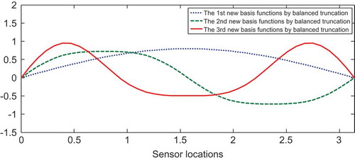
Figure 5. The first three combined basis functions by balancing of empirical Gramians for model reduction of Equation (23).

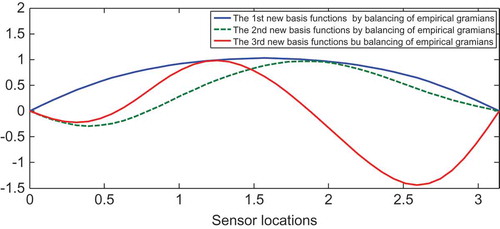
Figure 6. The distributed error based on three new spatial basis functions by balanced truncation method for model reduction of Equation (23).

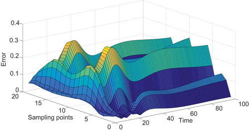
Figure 7. The distributed error based on three combined basis functions by balancing of empirical Gramians for model reduction of Equation (23).

4.2. Chaffee–Infante equation

The Chaffee–Infante equation was used as another numerical example in simulations. The Chaffee–Infante equation was introduced by Nathaniel Chaffee and Ettore Infante [44] as a typical reaction–diffusion equation. The mathematical model describing the spatio-temporal evolution with input consists of the following PDE:

(26) $\frac{\mathrm{\partial }X\left(z,t\right)}{\mathrm{\partial }t}=\frac{{\mathrm{\partial }}^{2}X\left(z,t\right)}{\mathrm{\partial }{z}^2}+\epsilon \left(X\left(z,t\right)-X{\left(z,t\right)}^3\right)+\sum _{i=1}^4{h}_i\left(z\right)u_i\left(t\right).$(26)

In this case, Equation (26) is subject to the following Dirichlet boundary and initial conditions:

(27) $X\left(0,t\right)=0,X\left(L,t\right)=0,X\left(z,0\right)=X_0\left(z\right),$(27)

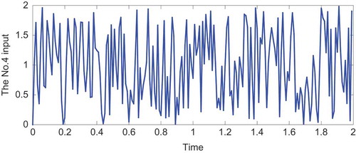
where $\mathrm{\Omega }=[0,L]$. $X(z,t)$ denotes the spatio-temporal variable. The parameter $\epsilon$ in model (26) was set as 1. Input $u_i(t)$ was available with the spatial distribution function $h_i(z)=H(z-\frac{(i-1)L}{4})-H((z-\frac{iL}{4}))$, where $i=1,2,3,4$, and $H(\cdot )$ is the standard Heaviside function. Input signals, $u_i(t)$, were random numbers selected from the uniform distribution (Figure 8). Suppose that 31 sensors uniformly distributed in the space were used for measurements. The sampling interval $\mathrm{\Delta }t$ was 0.01 s and the simulation time was 2 s. The values of the state variable at every time sampling for each sensor location were recorded, and a set of data was collected from Equation (26). The initial condition $X_0(z)$ was set to 0.

Figure 8. The No. 4 random temporal input of the Chaffee–Infante equation.

First, the input signals were set as random numbers generated from the uniform distribution and Equation (26) was computed using the finite difference method in the space domain [0,5] and time interval [0,2]. Spatial discretization of the PDE (26) was performed for 31 points and the interval of time discretization was 0.01 s. After the values for the boundaries of the space domain and initial time were determined, the values of the state variable for spatial discretization points were computed in accordance with the forward difference scheme. The temporal input signal $u_4(t)$ and corresponding measured spatio-temporal outputs for testing are shown in Figures 8 and 9, respectively.

Figure 9. The measured spatio-temporal output of Chaffee–Infante equation for testing.

Second, the spectral method was used for analysis of the model reduction in Equation (26) and spatial basis functions $\{\sqrt{2/L}sin(k\pi z/L),k=1,2,\cdots ,\mathrm{\infty }\}$ were used for time/space separation and Galerkin projection. According to the eigenspectrum of the spatial differential operator of the PDE (26), a small ratio factor $\tau =\left(\left|Re\left({\lambda }_1\right)\right|\right)/\left(\left|Re\left({\lambda }_N\right)\right|\right)$ was generally used for order determination, which results in a special $N$ value [20]. In calculations of empirical Gramians, the perturbation size of inputs was set as 0.10, and the initial condition of the states was set to be the steady state of the obtained finite-dimensional ODE system.

As shown in Figure 10, the RMSEs from the approximation models based on the three methods were compared. The RMSEs of the spectral-based model with different modes were initially calculated and the small ratio factor set to 0.1. Comparisons of eigenvalues revealed ${\lambda }_5$ was more than 10 times ${\lambda }_1$. Then, a spectral-based model with five modes was generally chosen to approximate the dominant dynamics of Equation (26). The RMSEs of the reduced model, which used the balanced truncation method with four modes, and the proposed method of balancing of empirical Gramians, which had two modes, were very similar to that of the spectral-based model with five modes. Specifically, a reduced model with four modes that uses the balanced truncation method can represent the dominant nonlinear dynamics of Equation (26). The reduced model, which involved balancing of empirical Gramians with two modes, sufficiently represented the dynamics of Equation (26). To describe the variances of the spatial basis functions, the first two new basis functions using the balanced truncation method and combined spatial basis functions involving balancing of empirical Gramians are shown in Figures 11 and 12, respectively. The distributed errors of the reduced models with two modes are presented in Figures 13 and 14, respectively.

Figure 10. Roots of mean square error based on spectral basis functions and two kinds of new spatial basis functions for model reduction of Chaffee–Infante equation.

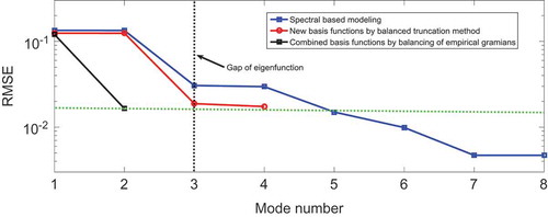
Figure 11. The first two new spatial basis functions by balanced truncation method for model reduction of Chaffee–Infante equation.

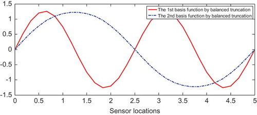
Figure 12. The first two combined spatial basis functions by balancing of empirical Gramians for model reduction of Chaffee–Infante equation.

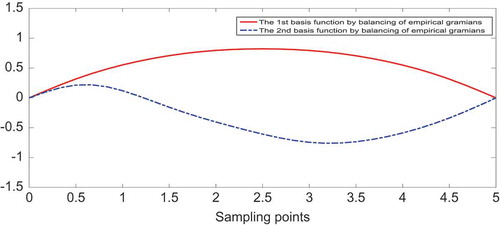
Figure 13. The approximated error based on two new spatial basis functions by balanced truncation method for model reduction of Chaffee–Infante equation.

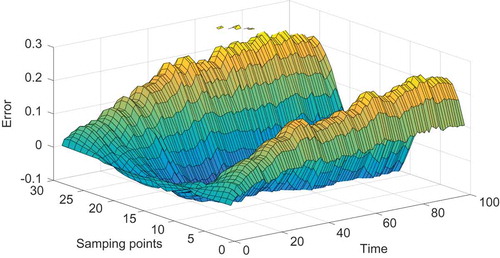
Figure 14. The distributed error based on two combined spatial basis functions by balancing of empirical Gramians for model reduction of Chaffee–Infante equation.

5. Conclusions

In this paper, empirical Gramians-based combined spatial basis functions were proposed for model reduction in nonlinear DPSs. Empirical Gramians were computed by generalizing linear Gramians for nonlinear systems. New spatial basis functions were obtained using linear combinations of the spectral eigenfunctions of DPSs, and matrices of combination coefficients were calculated by balancing empirical Gramians using standard matrix operations. Model reduction under the framework of Galerkin projection was performed for nonlinear DPSs. Two numerical examples were used to demonstrate the efficacy of the proposed approach. As for the linear Gramians-based combined spatial basis functions and spectral eigenfunctions-based model reduction, the reduced model with lower order was obtained within the given accuracy requirements.

Acknowledgements

This project was supported by the National Natural Science Foundation of China (Grant Nos. 51775182 and 51775181).

Disclosure statement

No potential conflict of interest was reported by the authors.

Additional information

Funding

This work was supported by the National Natural Science Foundation of China [51775182, 51775181]

References

- S. Munusamy, S. Narasimhan, and N.S. Kaisare, Order reduction and control of hyperbolic, countercurrent distributed parameter systems using method of characteristics, Chem. Eng. Sci. 110 (2014), pp. 153–163. doi:10.1016/j.ces.2013.12.029
- D.B. Pourkargar and A. Armaou, Geometric output tracking of nonlinear distributed parameter systems via adaptive model reduction, Chem. Eng. Sci. 116 (2014), pp. 418–427. doi:10.1016/j.ces.2014.05.030
- D.B. Pourkargar and A. Armaou, Modification to adaptive model reduction for regulation of distributed parameter systems with fast transients, AIChE J. 59 (12) (2013), pp. 4595–4611. doi:10.1002/aic.14207
- J.A. Rad, S. Kazem, and K. Parand, Optimal control of a parabolic distributed parameter system via radial basis functions, Commun. Nonlinear Sci. Numer. Simul. 19 (2014), pp. 2559–2567. doi:10.1016/j.cnsns.2013.01.007
- Y.Q. Ren, X.G. Duan, H.X. Li, and C.L. Philip Chen, Dynamic switching based fuzzy control strategy for a class of distributed parameter system, J. Process Control. 24 (2014), pp. 88–97.
- Y.Q. Ren, X.G. Duan, H.X. Li, and C.L. Philip Chen, Multi-variable fuzzy logic control for a class of distributed parameter systems, J. Process Control 23 (3) (2013), pp. 351–358. doi:10.1016/j.jprocont.2012.12.004
- S. Zheng, Z.X. Luo, Y.X. Deng, and H.C. Zhou, Development of a distributed-parameter model for the evaporation system in a supercritical W-shaped boiler, Appl. Thermal Eng. 62 (1) (2014), pp. 123–132. doi:10.1016/j.applthermaleng.2013.09.029
- C.K. Qi, H.X. Li, S.Y. Li, X.C. Zhao, and F. Gao, A fuzzy-based spatio-temporal multi-modeling for nonlinear distributed parameter processes, Appl. Soft. Comput. 25 (2014), pp. 309–321. doi:10.1016/j.asoc.2014.09.003
- C.K. Qi, H.X. Li, X.X. Zhang, X.C. Zhao, S.Y. Li, and F. Gao, Time/space separation based SVM modeling for nonlinear distributed parameter processes, Ind. Eng. Chem. Res. 50 (1) (2011), pp. 332–341. doi:10.1021/ie1002075
- M. Izadi and S. Dubljevic, Order-reduction of parabolic PDEs with time-varying domain using empirical eigenfunctions, AIChE J. 59 (11) (2013), pp. 4142–4150. doi:10.1002/aic.v59.11
- X.J. Lu, F. Yin, C. Liu, and M.H. Huang, Online spatiotemporal extreme learning machine for complex time-varying distributed parameter systems, IEEE Trans. Ind. Inform. 13 (4) (2017), pp. 1753–1762. doi:10.1109/TII.2017.2666841
- X.J. Lu, F. Yin, and M.H. Huang, Online spatiotemporal least-squares support vector machine modeling approach for time-varying distributed parameter processes, Ind. Eng. Chem. Res. 56 (25) (2017), pp. 7314–7321. doi:10.1021/acs.iecr.7b00984
- X.J. Lu, W. Zou, and M.H. Huang, A novel spatiotemporal LS-SVM method for complex distributed parameter systems with applications to curing thermal process, IEEE Trans. Ind. Inform. 12 (3) (2016), pp. 1156–1165. doi:10.1109/TII.2016.2557805
- P.D. Christofides (Ed), Special issue on ‘control of complex process systems’, Int. J. Robust Nonlinear Control. 14(2) (2004), pp. 87–88. doi:10.1002/(ISSN)1099-1239.
- P.D. Christofides and A. Armaou (eds.), Control of multi-scale and distributed process systems-preface, Comput. Chem. Eng. 29(4) (2005), pp. 687–688. doi:10.1016/j.compchemeng.2004.09.003.
- P.D. Christofides and X.Z. Wang (eds.), Special issue on ‘control of particulate processes’, Chem. Eng. Sci. 63(5) (2008), pp. 1155. doi:10.1016/j.ces.2007.07.025.
- F. Kwasniok, The reduction of complex dynamical systems using principal interaction patterns, Physica D 92 (1996), pp. 28–60. doi:10.1016/0167-2789(95)00280-4
- I.S. Sadek and M.A. Bokhari, Optimal control of a parabolic distributed parameter system via orthogonal polynomials, Optimal Control Appl. Methods 19 (3) (1998), pp. 205–213. doi:10.1002/(SICI)1099-1514(199805/06)19:3<205::AID-OCA613>3.0.CO;2-W
- P.D. Christofides, Nonlinear and Robust Control of PDE Systems: Methods and Applications to Transport-Reaction Processes, Birkhauser, Boston, 2001.
- H. Deng, H.X. Li, and G.-R. Chen, Spectral-approximation-based intelligent modeling for distributed thermal processes, IEEE Trans. Control Syst. Technol. 13 (5) (2005), pp. 686–700. doi:10.1109/TCST.2005.847329
- H.M. Park and D.H. Cho, The use of the Karhunen-Loeve decomposition for the modeling of distributed parameter systems, Chem. Eng. Sci. 51 (1996), pp. 81–98. doi:10.1016/0009-2509(95)00230-8
- H.M. Park and D.H. Cho, Low dimensional modeling of flow reactors, Int. J. Heat Mass Transf. 39 (16) (1996), pp. 3311–3323. doi:10.1016/0017-9310(96)00038-5
- A. Armaou and P.D. Christofides, Computation of empirical eigenfunctions and order reduction for nonlinear parabolic PDE systems with time-dependent spatial domains, Nonlinear Anal. 47 (4) (2001), pp. 2869–2874. doi:10.1016/S0362-546X(01)00407-2
- B. Luo, H.N. Wu, and H.X. Li, Data-based suboptimal neuro-control design with reinforcement learning for dissipative spatially distributed processes, Ind. Eng. Chem. Res. 53 (19) (2014), pp. 8106–8119. doi:10.1021/ie4031743
- M. Li and P.D. Christofides, Optimal control of diffusion-convection-reaction processes using reduced-order models, Comput. Chem. Eng. 32 (9) (2008), pp. 2123–2135. doi:10.1016/j.compchemeng.2007.10.018
- L.G. Bleris and M.V. Kothare, Low-order empirical modeling of distributed parameter systems using temporal and spatial eigenfunctions, Comput. Chem. Eng. 29 (4) (2005), pp. 817–827. doi:10.1016/j.compchemeng.2004.09.021
- F. Kwasniok, Optimal Galerkin approximation of partial differential equations using principal interaction patterns, Phys. Rev. E 55 (1997), pp. 5365–5375. doi:10.1103/PhysRevE.55.5365
- N. Aubry, W.Y. Lian, and E.S. Titi, Preserving symmetries in the proper orthogonal decomposition, SIAM J. Sci. Comput. 14 (1993), pp. 483–505. doi:10.1137/0914030
- D. Armbruster, R. Heiland, E.J. Kostelich, and B. Nicolaenko, Phase-space analysis of bursting behavior in Kolmogorov flow, Physica D 58 (1992), pp. 392–401. doi:10.1016/0167-2789(92)90125-7
- A. Chatterjee, An introduction to the proper orthogonal decomposition, Curr. Sci. 78 (7) (2000), pp. 808–817.
- M. Jiang and H. Deng, Optimal combination of spatial basis functions for the model reduction of nonlinear distributed parameter systems, Commun. Nonlinear Sci. Numer. Simul. 17 (2012), pp. 5240–5248. doi:10.1016/j.cnsns.2012.05.006
- H. Deng, M. Jiang, and C.Q. Huang, New spatial basis functions for the model reduction of nonlinear distributed parameter systems, J. Process Control 22 (2) (2012), pp. 404–411. doi:10.1016/j.jprocont.2011.12.008
- M. Jiang, X.J. Li, J.G. Wu, and G.B. Wang, A precision on-line model for the prediction of thermal crown in hot rolling processes, Int. J. Heat Mass Transf. 78 (2014), pp. 967–973. doi:10.1016/j.ijheatmasstransfer.2014.07.061
- A. Lall, J.E. Marsden, and S. Glavaski, A subspace approach to balanced truncation for model reduction of nonlinear control system, Int. J. Robust Nonlinear Control 12 (2002), pp. 519–535. doi:10.1002/rnc.657
- J. Hahn and T.F. Edgar, An improved method for nonlinear model reduction using balancing of empirical gramians, Comput. Chem. Eng. 26 (10) (2002), pp. 1379–1397. doi:10.1016/S0098-1354(02)00120-5
- B. Moore, Principal component analysis in linear systems: controllability, observability, and model reduction, IEEE Trans. Automatic Control 26 (1) (1981), pp. 17–32. doi:10.1109/TAC.1981.1102568
- J.M.A. Scherpen, Balancing for nonlinear systems, Syst. Control Lett. 21 (2) (1993), pp. 143–153. doi:10.1016/0167-6911(93)90117-O
- M.S. Tombs and I. Postlethwaite, Truncated balanced realization of stable, non-minimal state-space systems, Int. J. Control. 46 (1989), pp. 1319–1330.
- G.H. Golub and V.L. Cf (eds.), Matrix Computations, Johns Hopkins University Press, Washington, D.C., 1996.
- W.H. Ray, Advanced Process Control, Butterworths, NewYork, 1981.
- B. Haasdonk and M. Ohlberger, Reduced basis method for finite volume approximations of parametrized linear evolution equations, ESAIM: M2AN 42 (2) (2008), pp. 277–302. doi:10.1051/m2an:2008001
- C.L. Sun and J. Hahn, Nonlinear Model Reduction Routines for MATLAB, Available at http://homepages.rpi.edu/~hahnj/Model_Reduction/index.html.
- H. Deng, Z. Xu, and H.X. Li, A novel neural internal model control for multi-input multi-output nonlinear discrete-time processes, J. Process Control 19 (8) (2009), pp. 1392–1400. doi:10.1016/j.jprocont.2009.04.011
- Z.B. Li, Traveling Wave Solution of Nonlinear Mathematical Physics Equations, SCIENCEP, Beijing, 2008.