Multiscale modelling and splitting approaches for fluids composed of Coulomb-interacting particles

ABSTRACT

We consider fluids composed of Coulomb-interacting particles, which aremodelled by the Fokker--Planck equation with a collision operator.Based on modelling the transport and collision of the particles,we propose new, computationally efficient, algorithms based on splitting the equations of motion into a global Newtonian transport equation, where the effects of an external electric field are considered, and a local Coulomb interaction stochastic differential equation, which determinesthe new velocities of the particle. Two different numerical schemes, one deterministic and the other stochastic, as well as an Hamiltonian splitting approach, are proposed for coupling the interactionand transport equations. Results are presented for two- and multi-particle systems with different approximations for the Coulomb interaction.Methodologically, the transport part is modelled by thekinetic equations and the collision part is modelled bythe Langevin equations with Coulomb collisions.Such splitting approaches allow concentrating on different solver methodsfor each different part. Further, we solve multiscale problems involving an external electrostatic field.We apply a multiscale approach so that we can decompose the different time-scales of the transport and the collision parts.We discuss the benefits of the different splitting approaches and theirnumerical analysis.

KEYWORDS:

• Splitting methods
• stochastic differential equations
• Fokker–Planck equations
• particle simulations
• Coulomb collisions
• Langevin equation
• deterministic–stochastic splitting
• Hamiltonian splitting

1. Introduction

In this article, we propose a multiscale approach to model a Fokker–Planck equation with collision operator, with which we can decouple the transport and collision equations for the sake of a greater efficiency of the solution process, see [1]. Such modelling of fluids composed of Coulomb-interacting particles are important for simulating high plasma densities, see [1-3] and [4], or complex fluids, see [5] and [6], which are done by Fokker–Planck equations with collision terms. We treat the modelling equations that arise from plasma systems, where Coulomb collisions have a strong effect on the behaviour of the plasma, e.g. plasma processing [7] or inertial fusion [8]. For such a situation, the collision term can be modelled by a Langevin equation rather than a Boltzmann term, see [2] and [3]. Then, we apply to the two-body scattering model the Fokker–Planck equation with the Langevin operator, instead of the Boltzmann equation, see [9].

The particle transport and Coulomb collisions in a dilute (classical weakly coupled) plasma, are modelled by the following Fokker–Planck equation with collision term, see also [3]:

(1) $\frac{\mathrm{\partial }{f}_{\alpha }}{\mathrm{\partial }t}+\mathit{v}\cdot \frac{\mathrm{\partial }{f}_{\alpha }}{\mathrm{\partial }\mathbf{x}}+\frac{q_{\alpha }}{m_{\alpha }}[\mathbf{E}+\mathbf{v}\times \mathbf{B}]\cdot \frac{\mathrm{\partial }f}{\mathrm{\partial }\mathit{v}}==\frac{\mathrm{\partial }{f}_{\alpha }}{\mathrm{\partial }t}{|}_{coll},$(1)

where $f_{\alpha }(\mathbf{x},\mathbf{v})$ is the phase-space distribution function (density) of a charged plasma species $\alpha$ subjected to the electromagnetic field $(\mathbf{E},\mathbf{B})$. $q_{\alpha }$ is the charge and $m_{\alpha }$ is the mass of species $\alpha$. Further, $\frac{\mathrm{\partial }{f}_{\alpha }}{\mathrm{\partial }t}{|}_{coll}$ is the collision integral for the Coulomb forces, see [9].

The collision operator is given by Landau’s collision term, see [10] and [11]. This collision term gives the rate of change of the phase-space distribution function $f_{\alpha }(\mathbf{x},\mathbf{v})$ of a charged-particle species $\alpha$ (electron or ion) as follows:

(2) $\frac{\mathrm{\partial }{f}_{\alpha }}{\mathrm{\partial }t}{|}_{coll}==\frac{\mathrm{\partial }}{\mathrm{\partial }\mathbf{v}}\cdot \left[\pi q_{\alpha }^2\mathrm{\Lambda }\sum _{\beta }{q}_{\beta }^2\int [f_{\alpha }\frac{\mathrm{\partial }{f^{\prime }}_{\beta }}{\mathrm{\partial }{\mathbf{v}}^{\prime }}-{f^{\prime }}_{\beta }\frac{\mathrm{\partial }{f}_{\alpha }}{\mathrm{\partial }{\mathbf{v}}^{\prime }}]\frac{[u^{2}I-\mathbf{u}\mathbf{u}]}{{\mathit{u}}^3}{d}^3{\mathbf{v}}^{\prime }\right],$(2)

where the sum is over the indices $\beta$ of the species of charged plasma particles, the position is given by x, and the velocity by v. The time is $t$. $q_{\beta }$ is the charge of species $\beta$, $f_{\beta }^{\prime }(\mathbf{x},{\mathbf{v}}^{\prime })$ is the phase-space distribution function (density) of the charged plasma species $\beta$, the relative velocity is given by $\mathbf{u}=\mathbf{v}-{\mathbf{v}}^{\prime },\mathit{u}=\left|\mathbf{u}\right|$, and $\mathrm{\Lambda }$ is the Coulomb logarithm. The collision parameters (in vector notation), viz, the drag and diffusion coefficients, are derived from a classical theory of the screened Coulomb collision in the Fokker–Planck limit, see [12].

To simulate the Fokker–Planck equation with collisions (1), we apply particle-based kinetic plasma simulations, see [1,13]. Here, we have the problem that classical particle methods, like Particle-in-Cell (PIC) codes, fail: they can efficiently solve low-density plasma interactions but ignore collisions, see [3] and [14].

For such complex hydrodynamics problems, it is important to develop numerical methods, which take into account the global transport and the local collision behaviour. Since recent years, splitting approaches get more and more important, while we could split the problem with different physical motivations, e.g. dissipative, energy conserved and global/local motivation, see [1,15] and [16]. For the dissipative particle dynamics, the splitting approaches deal with decomposing the Langevin equations into a set of fluctuation-dissipation terms and solve each equation, see [16,17] and [18]. The energy conserved motivation concentrate on decomposing the Langevin equations with respect to energy conserved conditions, see [15,19] and [20].

We propose the global/local idea for an algorithm that is based on splitting the equations of motion into a global Newtonian transport equation, where the effects of an external electric field are considered, and a local Coulomb interaction stochastic differential equation, which determines the new particle velocities.

Such a splitting approach allows a more detailed modelling of the parts and allows more efficiently applying solver methods for each part, see [21] and [22]. We obtain the following benefits:

• Transport part: Here, we can apply a multiscale approach to solve the different timescales of the external electric field with more accuracy, see [1].

• Collision part: Here, we can apply an efficient so-called particle moment collision model to solve the collision part in a local frame with more efficiency, see [14].

Moreover, the splitting approach, which is also known as multi-particle collision (MPC) dynamics, see [5], or methodologically it is a Lie–Trotter splitting (AB splitting), see [23], can allow the numerical aspects to be improved by:

• Higher order splitting approaches, e.g., Strang splitting or Störmer–Verlet algorithms (ABA splitting), see [15] and [24].

• Higher order methods for the ordinary differential equations (ODEs) or stochastic differential equations (SDEs), e.g. Runge–Kutta methods for the ODEs, see [25], or the Milstein scheme for the SDEs, see [26].

For the multiscale approach, we employ regular expansions and resolve the different time scales of the electromagnetic field. While the electric potential field has attractive quadratic parts and repulsive impact parts, the decomposition into different scales allows treating each scale-dependent equation with different time-steps, see [1]. Based on our previous work in [1], we apply a non-constant strength of noise (non-constant diffusion), see [3]. Here, we apply more accurate solver strategies for the underlying SDEs, e.g. finer time-steps or higher-order approaches.

In addition, we present numerical efforts based on the reducing of the collision model to a reduced collision model. Such reductions in the time-consuming collision computations allow accelerating the algorithms.

The numerical test examples deal with realistic problems of plasma processing, see [27, 28] and [29]. Here, we present multi-particle simulations of ion–ion collisions, which are important in material processing, e.g. etching processes in thin layer depositions, see [30].

The outline of the present article is as follows. In Section 2, we discuss the multiscale model of the Fokker–Planck equation with Coulomb collisions. In Section 3, we discuss the different splitting approaches and collision algorithms. The numerical results are discussed in Section 4 and we conclude our results in Section 5. Additional derivations of the model and splitting algorithms are discussed in detail in the Appendices.

2. Modelling

The motivation is to simulate plasma problems related to higher energy levels and for regimes such that particle collisions are very important [11]. For such regimes, the collision term is important and we have to model the interactions of particle–particle collisions, see [10] and [31].

For other regimes with lower energy, as in gaseous or fluid materials, we could decouple the heavy (atoms, neutrons, protons) and light particles (electrons) and solve a two-fluid model within a continuous regime with the Boltzmann equations, see [7,32] and [33]. For such cases, a pure application of a continuum model, see [34] and [9], we deal with the transport phenomena and can neglect the collision phenomena.

Here, we propose a model related to the higher energy levels, which is done with particle models, that resolve the physical problem at the particle level. Such models consider all the particles, which means electrons, positions, etc., see also [35]. Therefore, we have modelled the transport of the particles (kinetic equations) and in addition, the interactions of the particles (collision equations), see [35]. We concentrate on two-body scattering models, while for such a situation, the Boltzmann equation has problems with the molecular forces, see [9]. Therefore, it is known that one should model such problems by the Fokker–Planck equation with a collision term, see [11]. The FP equation with collision term models more precisely the two-body scattering model with test and field particles, see [14]. The solution of the FP equation with collision term is a discretised solution of the underlying ODEs and SDEs of the particle trajectories, which can be split as follows:

• kinetic equation (transport of the particles), which resolves the characteristics of the particles,

• collision equation (explicit collision equation of the particles), which resolves the interactions of the particles.

Further, we have to consider a multiscale model in the transport part. Here we assume a multiscale explicit electrical field, which has to be decomposed into the different hierarchical equations, see [1]. Such multiscale models are important for plasma material processing to control ionized particles in an external electrostatic field, see [27] and [36].

In the following, we start with the full 6D FP equation with Coulomb collisions and present the basic splitting approach. Then, we model each part separately with the underlying ODEs and SDEs of the particle trajectories. Last, we derive the multiscale ODEs and SDEs with respect to the multiple different scales, which allows dealing with the non-linear dynamics, e.g. blow-up scales (impact oscillators) and also highly oscillating scales (harmonic oscillators), see [37] and [31].

2.1 The full 6D model

The full model equation is related to a six-dimensional phase-space ($\mathbf{x},\mathbf{v}$) system and is given for our applications in the following Fokker–Planck notation:

(3) $\frac{\mathrm{\partial }{f}_{\alpha }}{\mathrm{\partial }t}+\mathbf{v}\cdot \frac{\mathrm{\partial }{f}_{\alpha }}{\mathrm{\partial }x}+\frac{q_{\alpha }}{m_{\alpha }}[\mathbf{E}(\mathbf{x},ϵ)]\cdot \frac{\mathrm{\partial }{f}_{\alpha }}{\mathrm{\partial }\mathbf{v}}=\frac{\mathrm{\partial }{f}_{\alpha }}{\mathrm{\partial }t}{|}_{coll},$(3)

where $f_{\alpha }(\mathbf{x},\mathbf{v})$ is the phase-space distribution function (density) of the charged plasma species $\alpha$ subjected to a multiscale electric field $\mathbf{E}(\mathbf{x},ϵ)$. $\frac{\mathrm{\partial }{f}_{\alpha }}{\mathrm{\partial }t}{|}_{coll}$ is the collision integral for the Coulomb forces, which is given in Equation (2).

Here, we make the following modelling Assumptions 2.1.

Assumption 2.1 We assume that we are given the Fokker–Planck Equation (3) and assume that the collision operator is given as a Langevin equation, see [11].

Then, we assume the following treatment of the FP equation:

1. The Fokker–Planck equation with collision term can be split into a transport and a collision term. The AB splitting algorithm is presented in Algorithm 1.

Algorithm 1 AB splitting algorithm for coupling transport and collision of the plasma simulation

1: Input: $f_{\alpha }(t^0)$ are the initial distribution functions. The time grid is given by $t^n$ with $n=0,\dots ,\tilde{N}$. $t^0$ is the initial time and $t^{\tilde{N}}=T$ the ending time.

2: for $n=0,\dots ,\tilde{N}-1$ do

3: We have the time step $\mathrm{\Delta }t=t^{n+1}-t^n$.

4: We rewrite the FP equation (3) into a system of equations with

${\mathbf{f}}_{\alpha }=({\tilde{f}}_{\alpha },{\hat{f}}_{\alpha }{)}^t$ and the splitting approach is given by

(4) $\frac{\mathrm{\partial }{\mathbf{f}}_{\alpha }}{\mathrm{\partial }t}=A{\mathbf{f}}_{\alpha }+B{\mathbf{f}}_{\alpha },witht\in [t^n,t^{n+1}],$(4)

with initial condition ${\mathbf{f}}_{\alpha }(t^n)=\left(\begin{array}{c}{f}_{\alpha }(t^n)\\ {\tilde{f}}_{\alpha }(t^{n+1})\end{array}\right)$ and the operators $A=\left(\begin{array}{cc}-\mathrm{v}\cdot \frac{\mathrm{\partial }}{\mathrm{\partial }\mathrm{x}}-\frac{q_{\alpha }}{m_{\alpha }}[\mathbf{E}(\mathrm{x},ϵ)]\cdot \frac{\mathrm{\partial }}{\mathrm{\partial }v}& 0\\ 0& 0\end{array}\right)$ and $B=\left(\begin{array}{cc}0& 0\\ 0& \frac{\mathrm{\partial }}{\mathrm{\partial }t}{|}_{coll}\end{array}\right)$. The system of equations (4) is equation by equation, see 2 and 3 in Assumption 2.1. The solution is ${\mathbf{f}}_{\alpha }(t^{n+1})=({\tilde{f}}_{\alpha }(t^n),{\hat{f}}_{\alpha }(t^{n+1}){)}^t$.

5: We update $f(t^{n+1})={\hat{f}}_{\alpha }(t^{n+1})$

6: end for

7: The output is given by $f_{\alpha }(t^n)$ and $n=1\dots ,\tilde{N}$.

• (2) The characteristics of the FP equation, meaning the transport part, are modelled with Cartesian coordinates; this is discussed in subsection 2.1.1.

• (3) The characteristics of the collision term (Langevin equation) are modelled with spherical coordinates. The derivation is discussed in subsection 2.1.2.

• (4) The models are coupled via splitting methods and we assume we can transform the solution in Cartesian coordinates into a solution in spherical coordinates and vice versa.

Remark 2.1 The characteristic parts are also solved with numerical methods, see [38] and [39]. The numerical solutions of each part can also be obtained via a splitting approach, see [40] and the underlying numerical errors can be derived, see [22]. Further, there are mappings between the Cartesian coordinates and the spherical coordinates and back, see [41].

2.1.1 Model of the transport part

The model of the transport part is given as the FP equation:

(5) $\frac{\mathrm{\partial }{f}_{\alpha }}{\mathrm{\partial }t}+\mathbf{v}\cdot \frac{\mathrm{\partial }{f}_{\alpha }}{\mathrm{\partial }\mathbf{x}}+\frac{q_{\alpha }}{m_{\alpha }}\mathbf{E}(\mathbf{x},ϵ)\cdot \frac{\mathrm{\partial }{f}_{\alpha }}{\mathrm{\partial }\mathbf{v}}=0,$(5)

where $f_{\alpha }$ is the density function of the particle $\alpha$. For the electrical field, we have the following functions:

(6) $\mathbf{E}(\mathrm{x},ϵ))=\left(\begin{array}{c}{ϵ}_x{E}_{1,x}(x)+E_{2,x}x={ϵ}_x\frac{2}{x^2}-2x,\\ {ϵ}_y{E}_{1,y}(y)+E_{2,y}x={ϵ}_y\frac{2}{y^2}-2y,\\ {ϵ}_z{E}_{1,z}(z)+E_{2,z}x={ϵ}_z\frac{2}{z^2}-2z,\end{array}\right),$(6)

where ${ϵ}_x,{ϵ}_y,{ϵ}_z\in [0,1]$ and $E_{1,x},E_{1,y},E_{1,z}:\mathrm{I}{\mathrm{R}}^{+}\to \mathrm{I}\mathrm{R}$ are non-linear functions. We have a singular electric field for ${ϵ}_x={ϵ}_y={ϵ}_z=1$, which blows up for $(x,y,z)\to (0,0,0)$. Such a problem is also called an impact oscillator [42]. Further, we have a linear electric field for ${ϵ}_x={ϵ}_y={ϵ}_z=0$, this problem is known as an harmonic oscillator. Based on such a singular part in the electrical field, we have employed a multiscale model, which allows separating the linear and non-linear E-fields and controls the blow-up behaviour, see the ideas in [42] and [13].

The characteristics of the FP equation are given in following multiscale kinetic equations:

(7) $\frac{d\mathrm{x}}{dt}=\mathbf{v},$(7)

(8) $\frac{d\mathbf{v}}{dt}=\frac{q_{\alpha }}{m_{\alpha }}\mathbf{E}(\mathbf{x},ϵ),$(8)

where we model the multiscale electric field in Section 2.2. The multiscale model deals with different time scales of the electromagnetic field, see [1], which model non-singular and singular electrical field effects, see [42].

2.1.2 Model of the collision part

For the collision part, we deal with a stochastic differential equation (Langevin equation). Here, we transform to a spherical coordinate system. In such a laboratory system, we can deal with so called test particles, which are considered in the SDE with drag and diffusion coefficients. Such particles influence the field particles of our original system and we could add the characteristics of the collision to our field particles, see [3]. The idea is based on the fact that the drag and diffusion coefficients for the test particle Coulomb scattering with the distribution of the field particles correspond to the drag and diffusion coefficients given in Equation (2), see [3].

Such collision terms in Equation (2) can be explicitly transformed to spherical coordinates, so that we have $v,\mu =cos(\theta ),\varphi$, where $v$ is the velocity in spherical coordinates, $\theta$ is the angle to the axial direction and $\varphi$ is the angle of the azimuthal direction.

The collision term of the field-test particle equations are given in the following, see [3,14,43] and [44]:

(9) $\frac{\mathrm{\partial }{f}_t}{\mathrm{\partial }t}{|}_{coll}=-\frac{\mathrm{\partial }}{\mathrm{\partial }v}(F_d(v)f_t)+\frac{{\mathrm{\partial }}^2}{\mathrm{\partial }{v}^2}(D_v(v)f_t)+\frac{\mathrm{\partial }}{\mathrm{\partial }\mu }(2D_a(v)\mu f_t)+\frac{{\mathrm{\partial }}^2}{\mathrm{\partial }{\mu }^2}(D_a(v)[1-{\mu }^2]f_t)+\frac{{\mathrm{\partial }}^2}{\mathrm{\partial }{\varphi }^2}(\frac{D_a(v)}{[1-{\mu }^2]}{f}_t),$(9)

where $f_t$ is the distribution function (density) of the test particles in the spherical coordinates. Further, the functions of the convection (drag force $F_d(v)$) and the velocity and angular diffusion (diffusion coefficients $D_v(v)$ and $D_a(v)$) are given by

(10) $F_d(v)=-\frac{A_D}{2v^2}\left[\left[[1+\frac{m_t}{m_f}]2l_f^2{v}^2+1\right]G(l_{f}v)-\mathrm{\Phi }(l_{f}v)\right],$(10)

(11) $D_v(v)=\frac{A_D}{2v^2}G(l_{f}v),$(11)

(12) $D_a(v)=\frac{A_D}{4v^3}\left[\mathrm{\Phi }(l_{f}v)-G(l_{f}v)\right],$(12)

where we have the following functions and parameters:

(13) $A_D=\frac{8\pi n_f{q}_t^2{q}_f^2\lambda }{m_f^2}2v^2,$(13)

(14) $G(x)=\frac{\mathrm{\Phi }(x)-x{\mathrm{\Phi }}^{\prime }(x)}{2x^2},$(14)

where $x=l_{f}v$, $l_f=\frac{1}{\sqrt{2}{v}_f}$, $v_f=\sqrt{\frac{T_f}{m_f}}$, $ln\mathrm{\Lambda }$ is the Coulomb logarithm, and $\mathrm{\Phi }$ is the error function. Further, $n_f$ is the field particle density, $T_f$ is the field particle temperature and $m_t$ and $m_f$ are the test and field particle masses.

Equation (9) is given in the form of the FP equation for a three-dimensional SDE system with drag and diffusion coefficients, see [3]. Such a notation depends on the variables in the Ito calculus, see [39] and [45]. Therefore, the Fokker–Planck equation corresponds to a forward explicit discretization scheme, e.g. an Euler–Maruyama or Milstein scheme, see [46,47] and [48]. Then, the resulting three dimensional SDE system is given by

(15) $dv(t)=F_d(v)dt+\sqrt{2D_v(v)}d{W}_v(t),$(15)

(16) $d\mu (t)=-2D_a(v)\mu dt+\sqrt{2D_a(v)[1-{\mu }^2]}d{W}_{\mu }(t),$(16)

(17) $d\varphi (t)=\sqrt{\frac{2D_a(v)}{[1-{\mu }^2]}}d{W}_{\varphi }(t),$(17)

where $W_v,W_{\mu },W_{\varphi }$ are independent Wiener processes, i.e. stochastic processes with centred Gaussian increments that are independent for non-overlapping time intervals.

2.2 Multiscale modelling

We deal with a multiscale model that is derived in Appendix 1, which gives us the modelling equation

(18) $\frac{\mathrm{\partial }f}{\mathrm{\partial }t}+v\frac{\mathrm{\partial }f}{\mathrm{\partial }x}+E(x,ϵ)\frac{\mathrm{\partial }f}{\mathrm{\partial }v}=\frac{\mathrm{\partial }}{\mathrm{\partial }v}(-F_d(v)f+\frac{\mathrm{\partial }}{\mathrm{\partial }v}(D_v(v)f)).$(18)

We have to model the multiscale term, which is related to the multiscale operator $E(x,ϵ)$, which is given in a one-dimensional notation. Such electrostatic fields are related to models based on plasma apparatus simulations, see [29]. Based on the non-linear dynamics of such an electrostatic field, our considerations are also related to those of such problems as oscillators, see [42] and [49].

The underlying electrostatic potential is given by

(19) $U(x,ϵ)=ϵ\frac{1}{x^2}+x^2$(19)

where $ϵ\in [0,1]$ and $E(x,ϵ)=-\frac{\mathrm{\partial }}{\mathrm{\partial }x}U(x,ϵ)$. The potential consists of an attractive quadratic part and a repulsive impact part. Such problems can also be studied as non-linear dynamical systems, see [49]. We consider a modelling based on regular scale expansion methods. Such methods are known to be flexible and have solutions depending simultaneously on widely different scales, see [50] and [51].

In the following, we derive the deterministic and stochastic parts of the multiscale characteristics, see also [1].

2.2.1 Regular expansion of the deterministic part

The Fokker–Planck equation without the collision part is given by

(20) $\frac{\mathrm{\partial }f}{\mathrm{\partial }t}+v\frac{\mathrm{\partial }f}{\mathrm{\partial }x}+E(x,ϵ)\frac{\mathrm{\partial }f}{\mathrm{\partial }v}=0,$(20)

and the multiscale trajectories based on the multiscale electrostatic field, see also [11 ] and [53], are given by

(21) $\frac{dx(t,ϵ)}{dt}=v(t,ϵ),\frac{dv(t,ϵ)}{dt}=E(x,ϵ).$(21)

The multiscale electrostatic field is a typical example, with mixtures of different oscillatory solutions, i.e. harmonic and impact oscillations, over time scales that are greater than the period of the known oscillations, see [54].

Based on our problem, we have a mixture of a harmonic oscillator and an impact oscillator:

(22) $E(x,ϵ)=ϵE_1(x)+E_{2}x,$(22)

where $E_1(x)$ is the non-linear part and we have an impact oscillator $E_1(x)=\frac{2}{x^3}$. Further, the linear part, which is given by $E_{2}x=-2x$, is a harmonic oscillator, see [42].

We assume a regular perturbation expansion, and apply the following underlying idea, see [55] and [56]. For $x(t,ϵ)$ and $v(t,ϵ)=\frac{dx(t,ϵ)}{dt}$, we have

(23) $x(t,ϵ)=x_0(t)+ϵx_1(t)+{ϵ}^2{x}_2(t)+\dots +{ϵ}^J{x}_J(t),$(23)

(24) $\frac{dx(t,ϵ)}{dt}=\frac{d{x}_0(t)}{dt}+ϵ\frac{d{x}_1(t)}{dt}+{ϵ}^2\frac{d{x}_2(t)}{dt}+\dots +{ϵ}^J\frac{d{x}_J(t)}{dt},$(24)

where $ϵ\in [0,1]$ and $J$ is a number related to the order of the expansion. Such a flexibilization allows solving each term of the equation with the optimal time scale, see [1].

The regular expansion of the multiscale electrostatic field $E(x,ϵ)$ is given by

• The non-linear operator is given by

(25) $E_1(x(t,ϵ))=E_1(x_0(t)+ϵx_1(t)+{ϵ}^2{x}_2(t)+\dots +{ϵ}^J{x}_J(t))=E_1(x_0(t))+\frac{d{E}_1}{dx}{|}_{x=x_0}(ϵx_1(t)+{ϵ}^2{x}_2(t)+\dots +{ϵ}^J{x}_J(t))+\frac{d^2{E}_1}{d{x}^2}{|}_{x=x_0}\frac{{(ϵx_1(t)+{ϵ}^2{x}_2(t)+\dots +{ϵ}^J{x}_J(t))}^2}{2!}+\dots ,$(25)

where we have a blow-up with $\left|\left|E_1(0)\right|\right|\to \mathrm{\infty }$ with $ϵ\to 1$.

• The linear operator is given by

(26) $E_2(x(t,ϵ))=E_2{x}_0(t)+ϵE_2{x}_1(t)+$(26)

$+{ϵ}^2{E}_2{x}_2(t)+\dots +{ϵ}^J{E}_2{x}_J(t).$

Then, we apply the regular scale extensions to the ODEs (31) and obtain

(27) $\begin{array}{rl}& \frac{d{x}_0(t)}{dt}+ϵ\frac{d{x}_1(t)}{dt}+v^2\frac{d{x}_2(t)}{dt}+\dots =v_0+ϵv_1+{ϵ}^2{v}_2\\ & +\dots \frac{d{v}_0(t)}{dt}+ϵ\frac{d{v}_1(t)}{dt}+{ϵ}^2\frac{d{v}_2(t)}{dt}+\dots \\ & =ϵ\left(E_1(x_0)+\frac{d{E}_1}{dx}{|}_{x=x_0}(ϵx_1+\dots +{ϵ}^J{x}_J)+\frac{d^2{E}_1}{d{x}^2}{|}_{x=x_0}\frac{{(ϵx_1+\dots +{ϵ}^J{x}_J)}^2}{2!}+\dots \right)\\ & +E_2(x_0(t)+ϵx_1(t)+\dots +{ϵ}^J{x}_J(t)).\end{array}$(27)

The multiscale ODE system for the deterministic part is given by

(28) $\frac{d{x}_0(t)}{dt}=v_0,\frac{d{x}_1(t)}{dt}=v_1,$(28)

(29) $\frac{d{v}_0(t)}{dt}=E_2{x}_0(t),\frac{d{v}_1(t)}{dt}=E_1(x_0(t))+E_2{x}_1(t).$(29)

where we have a first order approach in $ϵ$, see [57].

2.2.2 Regular expansion of the stochastic part

The collision part of the Fokker–Planck equation is

(30) $\frac{\mathrm{\partial }f}{\mathrm{\partial }t}{|}_{coll}=\frac{\mathrm{\partial }}{\mathrm{\partial }v}(-F_d(v)f+\frac{\mathrm{\partial }}{\mathrm{\partial }v}(D_v(v)f)),$(30)

and the multiscale trajectories based on the multiscale SDE with drag and diffusion coefficients, depending on the Ito calculus, see also [3], satisfy

(31) $dv(t,ϵ)=F_d(v)dt+\sqrt{2D_v(v)}d{W}_v.$(31)

We apply the regular scale extensions for the $v$ variable and obtain

(32) $d(v_0+\dots +{ϵ}^J{v}_J)=F_d(v_0+\dots +{ϵ}^J{v}_J)dt+\sqrt{2D(v_0+\dots +{ϵ}^J{v}_J)}d{W}_{v_0+\dots +{ϵ}^J{v}_J}(t),$(32)

where we have $\tilde{D}(v_0+\dots +{ϵ}^J{v}_J)(v_0+\dots +{ϵ}^J{v}_J)=\sqrt{2D_v(v_0+\dots +{ϵ}^J{v}_J)}s$. Further, we assume that the independent Wiener processes are not influenced by the multiscale effects, which means we have ${ϵ}^{j}d{W}_v(t)={ϵ}^{j}d{W}_{v_j}(t)$ for $j=1,\dots ,J$, see [39].

Therefore, we employ the following notation, that the multiscale equations with the scale-dependent SDE with $d{v}_0,v_1,\dots ,d{v}_J$ have independent Wiener processes. The processes are given by $d{W}_j=\sqrt{dt}{\xi }_j$ with $\varphi (t^{n+1})=\tilde{\varphi }(t^{n+1})+\sqrt{\frac{2D_a(\tilde{v}(t^{n+1}))}{(1-\tilde{\mu }{(t^{n+1})}^2)}}\mathrm{\Delta }{W}_{\varphi },$ independently normally distributed random variables with $⟨{\xi }_j⟩=0$, $⟨{\xi }_j^2⟩=1$ for $j=1,\dots ,J$. We apply the Taylor expansion to the non-linear operators and obtain

• The drag operator is given by

$F_d(v(t,ϵ))=F_d(v_0(t))+\frac{d{F}_d}{dv}{|}_{v=v_0}(ϵv_1(t)+{ϵ}^2{v}_2(t)+\dots +{ϵ}^J{v}_J(t))+$

$+\frac{d^2{F}_d}{d{v}^2}{|}_{v=v_0}\frac{{(ϵv_1(t)+{ϵ}^2{v}_2(t)+\dots +{ϵ}^J{v}_J(t))}^2}{2!}+\dots .$

(33) $=F_d(x_0(t))+ϵ\frac{d{F}_d(v)}{dv}{|}_{v=v_0}(v_1(t))+\dots .$(33)

• The diffusion operator is given by

(34) $\sqrt{2D(v(t,ϵ))}=\sqrt{2D(v_0(t)}+\frac{d(2D)}{dv}{|}_{v=v_0}(ϵv_1(t)+{ϵ}^2{v}_2(t)+\dots +{ϵ}^J{v}_J(t))+\frac{d^2(2D)}{d{v}^2}{|}_{v=v_0}\frac{{(ϵv_1(t)+{ϵ}^2{v}_2(t)+\dots +{ϵ}^J{v}_J(t))}^2}{2!}+\dots =\sqrt{2D(v_0(t)}+ϵ\left({\left(2D(v)\right)}^{-1/2}\frac{dD(v)}{dv}\right){|}_{v=v_0}{v}_1(t)+\dots$(34)

The multiscale SDE system for the deterministic part is given by

(35) $d{v}_0=F_d(v_0(t))dt+\sqrt{2D(v_0(t))}d{W}_{v_0}(t),$(35)

(36) $d{v}_1=\frac{d{F}_d(v)}{dv}{|}_{v=v_0}{v}_{1}dt+\left({\left(2D(v)\right)}^{-1/2}\frac{dD(v)}{dv}\right){|}_{v=v_0}{v}_{1}d{W}_{v_1}(t),$(36)

where we have a first order approach in $ϵ$, see [57].

3. Solver method

In the following, we discuss the solver methods for the particle equations, which are coupled transport Equations (28) and (29) and collision Equations (35) and (36).

In the literature, there are three general methods for solving such coupled plasma kinetic equations with collisions:

1. A continuum method on an Eulerian grid (phase-space grid), see [58] and [59].

2. A particle approach using a Lagrangian formulation, see [60] and [61].

   1. Some methods that mix the two formulations, e.g. semi-Lagrangian methods, see [62] and [63].

We concentrate on the second approach and consider the collision in spherical polar coordinates (relative to the individual particle velocity before the collision), see [14]. The transport or the rest of the kinetic equation in Cartesian coordinates consists of

1. an acceleration of the velocity vector and

2. the advection of the particle along the particle characteristics in phase-space.

We propose for such a treatment a splitting of these physical processes, where we employ the different coordinate systems, and split them into:

• a transport term (Cartesian coordinates), which means the global Newtonian transport equation, and

• a collision term (spherical coordinates), which means the local Coulomb interaction stochastic differential equation.

In passing between the two coordinate systems, we have to transform the spherical velocity coordinates to the Cartesian velocity coordinates in applying the acceleration due to the electromagnetic fields to each particle. Further, we have to transform the Lorentz force/acceleration onto the spherical velocity coordinate of each particle.

Here, we consider a simplified particle–particle model, so that we can circumvent the many-particle approaches, where we have to keep in mind that the solution of the Maxwell equations involves currents obtained from the particles in a common coordinate scheme. Hence, the velocity/displacement advection from which the currents are computed are most conveniently done in the same common coordinate scheme, see [2] and [14].

Further, for the Coulomb collisions, there are two algorithms in particle simulations, which employ finite-sized particles:

• The binary algorithm: The particles interact in a finite cell (e.g., particle-in-cell (PIC) simulation), where they are organised into discrete pairs of interacting particles. The collisions are based on the scattered velocities and angle of the particles and we apply a statistical variance by the theory of Coulomb collisions, see [12] and [64].

• The test particle algorithm: Here, the collision is based on defining test and field particles, which interact. The velocity and the angle of the test particle are modelled by the Langevin equations (stochastic equations) with drag and diffusion coefficients. The test particles influence the moments of the field particle and their velocity and angle distributions. Such results are given on the spatial mesh [14,31,60,65] and [66].

We concentrate on the second idea, that of the collision algorithms, and deal with stochastic differential equations, see [1,2,67] and [14].

The underlying idea of the multi-particle collision algorithm is that it can be decomposed into a streaming step and a collision step. The basic ideas are given in Algorithm 2.

Algorithm 2 Basic MPC Algorithm

1: Input: ${\mathbf{x}}_i(t),{\mathbf{v}}_i(t)$ are the spatial- and velocity-coordinates of the particles, $i=1,\dots ,N$. Further, we have the global time-step and $\mathrm{\Delta }t$.

2: Streaming step (Transport step) in the common (global) coordinate system:

(37) ${\mathbf{x}}_i(t+\mathrm{\Delta }t)={\mathbf{x}}_i(t)+{\mathbf{v}}_i(t)\mathrm{\Delta }t.$(37)

3: Collision step (local interaction of the particles) in the local coordinate system: The particles are sorted into collision cells (local coordinate systems) and updated by the following collision step:

(38) ${\mathbf{v}}_i(t+\mathrm{\Delta }t)={\mathbf{v}}_f(t)+\hat{R}({\mathbf{v}}_j(t)-{\mathbf{v}}_f(t)),$(38)

where ${\mathbf{v}}_f(t^n)$ is the centre of the mass-velocity of the particles in the local coordinate system and $\hat{R}$ is the rotation matrix. $\hat{R}$ includes the performed rotation by an angle $\alpha$ around a random rotation axis, which means we express the drag and diffusion coefficients, see also [68].

4: The output is given by ${\mathbf{x}}_i(t^{n+1}),{\mathbf{v}}_i(t^{n+1})$ are the spatial- and velocity-coordinates of the particles with $i=1,\dots ,N$.

3.1 MPC algorithm for coupling the transport and collision parts

In the following, we present the coupled model based on the following splitting model idea:

• We consider a common coordinate system, which is a Cartesian system. In this system, we consider the transport of the so-called field particles.

• We choose one particle of the field particles to be the test particle.

• We choose an average of the field particles with the velocity ${\mathbf{v}}_f$.

• We shift to a local coordinate system in which the average velocity of the chosen field particle vanishes, and we have the test velocity ${\mathbf{v}}_t-{\mathbf{v}}_f$ transported with ${\mathbf{v}}_t$, ${\mathbf{v}}_f$ in the common coordinate system.

• We scatter the test particle in the local coordinate system, which is a spherical coordinate system.

• All the previous steps are done with each particle in turn being the test particle.

• Then we shift the scattered velocity back to the Cartesian coordinate system (the common coordinate system) and we calculate the increment $\mathrm{\Delta }{\mathbf{v}}_i$ of each particle.

• For multiple particles, we have to shift the velocity $\mathrm{\Delta }{\mathbf{v}}_i$ in such a way that the total momentum and energy are conserved, see also [14].

In the following, we assume, without loss of generality, that there are two particles, a field particle and a test particle. The algorithm is also known as the multiparticle collision dynamics (MPC) algorithm, where the collision step also includes an electromagnetic interaction part, see [5] and [6].

The algorithm is presented in 3.

Algorithm 3 MPC Algorithm for Coupling Transport and Collision of the Plasma-simulation

• 1: Input: ${\mathbf{x}}_i(t^0),{\mathbf{v}}_i(t^0)$ are the spatial- and velocity-coordinates of the particles, $i=1,\dots ,N$, $N$ is the number of particles. $t^n$, for $n=0,\dots ,\tilde{N}$, are the time-points, $t^0$ is the initial time, and $t^{\tilde{N}}$ is the ending time.

• 2: for $n=0,\dots ,\tilde{N}-1$ do

  • 3: We have the time-step and $\mathrm{\Delta }t=t^{n+1}-t^n$. Transport step in the common (global) coordinate system:

(39) $\frac{d{\tilde{\mathrm{x}}}_i(t)}{dt}={\tilde{\mathrm{v}}}_i(t),\frac{d{\tilde{\mathrm{v}}}_i(t)}{dt}=\mathbf{E}({\tilde{\mathrm{x}}}_i(t),ϵ)t\in [t^n,t^{n+1}],$(39)

with initial conditions ${\tilde{\mathrm{x}}}_i(t^n)={\mathrm{x}}_i(t^n)$, ${\tilde{\mathrm{v}}}_i(t^n)={\mathrm{v}}_i(t^n)$ and the solutions ${\mathrm{x}}_i(t^{n+1})$, ${\mathrm{v}}_i(t^{n+1})$ are obtained by applying an ODE solver.

• 4: for $\tilde{i}=1,\dots ,N$ do

• 5: Step A (test particle and field particle): The average field particle is given in the common coordinate system:

(40) ${\mathbf{v}}_f(t^{n+1})=\frac{\sum _{j=1,j\ne \tilde{i}}^N{{\tilde{\mathbf{v}}}_j}_j(t^{n+1})}{N},$(40)

where ${\mathbf{v}}_t(t^{n+1})={\tilde{\mathbf{v}}}_{\tilde{i}}(t^{n+1})$ is the velocity of the test particle and we assume there are $N$ particles.

6: Transformation step: Common to local coordinate system

(41) $v=\sqrt{v_{local,x}^2+v_{local,y}^2+v_{local,z}^2},$(41)

(42) $\theta =\mathrm{a}\mathrm{r}\mathrm{c}\mathrm{c}\mathrm{o}\mathrm{s}\left(\frac{v_{local,z}}{v}\right),\varphi =\mathrm{a}\mathrm{r}\mathrm{c}\mathrm{t}\mathrm{a}\mathrm{n}\left(\frac{v_{local,y}}{v_{local,x}}\right),$(42)

$\mathrm{w}\mathrm{h}\mathrm{e}\mathrm{r}\mathrm{e}{\mathbf{v}}_{local}(t^{n+1})={\mathbf{v}}_t(t^{n+1})-{\mathbf{v}}_f(t^{n+1})\mathrm{a}\mathrm{n}\mathrm{d}{\mathbf{v}}_{local}(t^{n+1})=(v_{local,x}(t^{n+1}),v_{local,y}(t^{n+1}),v_{local,z}(t^{n+1}){)}^t.$

Further, we make the transformation $\tilde{\mu }(t^{n+1})=cos(\tilde{\theta }(t^{n+1}))$.

7: Step B (Collision of the field and test particles in the local coordinate system, i.e., spherical coordinates):

(43) $dv(t)=F_d(v)dt+\sqrt{2D_v(v)}d{W}_v(t),$(43)

(44) $d\mu (t)=-2D_a(v)\mu dt+\sqrt{2D_a(v)(1-{\mu }^2)}d{W}_{\mu }(t),$(44)

(45) $d\varphi (t)=\sqrt{\frac{2D_a(v)}{(1-{\mu }^2)}}d{W}_{\varphi }(t),$(45)

with initial conditions $v(t^n)=\tilde{v}(t^n)$, $\mu (t^n)=\tilde{\mu }(t^n)$, $\varphi (t^n)=\tilde{\varphi }(t^n)$ and the solutions $v(t^{n+1})$, $\mu (t^{n+1})$, $\varphi (t^{n+1})$ are obtained by applying an SODE solver. We transform $\theta (t^{n+1})=\mathrm{a}\mathrm{r}\mathrm{c}\mathrm{c}\mathrm{o}\mathrm{s}(\mu (t^{n+1}))$.

8: Transformation step: Local to common coordinate system

(46) ${\mathbf{v}}_t(t^{n+1})={\mathbf{v}}_f+\left(\begin{array}{ccc}cos(\theta (t^n))cos(\varphi (t^n))& -sin(\varphi (t^n))& sin(\theta (t^n))cos(\varphi (t^n))\\ cos(\theta (t^n))sin(\varphi (t^n))& cos(\varphi (t^n))& sin(\theta (t^n))sin(\varphi (t^n))\\ -sin(\theta (t^n))& 0& cos(\varphi (t^n))\\ \hspace{0.17em}& \hspace{0.17em}& \hspace{0.17em}\end{array}\right)\cdot \left(\begin{array}{c}(v(t^n)+\mathrm{\Delta }v)sin(\mathrm{\Delta }\theta )cos(\mathrm{\Delta }\varphi )\\ (v(t^n)+\mathrm{\Delta }v)sin(\mathrm{\Delta }\theta )sin(\mathrm{\Delta }\varphi )\\ (v(t^n)+\mathrm{\Delta }v)cos(\mathrm{\Delta }\varphi )\\ \hspace{0.17em}\end{array}\right),$(46)

with $\mathrm{\Delta }\varphi =\varphi (t^{n+1})-\varphi (t^n)$, $\mathrm{\Delta }\theta =\theta (t^{n+1})-\theta (t^n)$ and $\mathrm{\Delta }v=v(t^{n+1})-v(t^n)$.

9: Shift of the $\tilde{i}$th particle in the common coordinate system:

(47) $\mathrm{\Delta }{\mathbf{v}}_t={\mathbf{v}}_t(t^{n+1})-{\mathbf{v}}_t.$(47)

• 10: The result is given by ${\mathbf{x}}_{\tilde{i}}(t^{n+1})={\mathbf{x}}_t(t^{n+1}),{\mathbf{v}}_{\tilde{i}}(t^{n+1})={\mathbf{v}}_t(t^{n+1})$.

• 11: end for

• 12: end for

• 13: The output is given by ${\mathbf{x}}_i(t^n),{\mathbf{v}}_i(t^n)$ are the spatial- and velocity-coordinates of the particles with $i=1,\dots ,N$ and $n=1\dots ,\tilde{N}$.

In the following, without loss of generality, we concentrate on a 2D model and discuss different splitting models and the underlying long time conservation analysis (symplecticity). Based on the specific results in the 2D model, we can later upscale the results to the 6D model. Such an up-scaling is possible due to the linearity of the dependencies, see [11].

3.2 Modification of the MPC algorithm

Based on the MPC algorithm, which is presented for our applications in Algorithm 3, we discuss a novel treatment to accelerate or improve the accuracy of such a method.

The improvements of the MPC algorithm are in two directions:

• Algorithmically: The main problem of the algorithm is based on the lower order splitting approach in the transport step. Here, we deal with a simple AB splitting or semi-implicit Euler method, see [15] and [23].

We improve this with higher order splitting approaches, as follows:

• Deterministic–Stochastic ABA or Strang splitting approach: We decompose into three steps, namely, first the A-step (transport step) with fast ODE solvers, second the B-step (collision step) with SDE solvers, which can be done with a more accurate and finer local time-step, and third, an A-step (transport step) with the fast ODE solver, see the schemes in Appendix 2.2.

• Hamiltonian ABA or Störmer–Verlet splitting approach: We decompose into three steps, which means first an A-step (x-variable step) with a fast explicit Euler method (ODE solver), second, a B-step (v -variable step) with a fast Euler–Maruyama method (SDE solver), and third, an A-step (x -variable step) with a fast explicit Euler method (ODE solver), see the schemes in Appendix 2.3.

All derivations and ideas are explained in Appendix 2.

• Methodologically: A methodological problem arises from the single-scale modelling equations. Here the improvements are based on multiscale modelling equations, which allow more accurately modelled problems.

  • Multiscale modelling of the FP equation with collision term: We apply a multiscale approach to the modelling equation and improve the accuracy, see the modelling approaches in Appendix 1.2.

  • The standard collision model applied often reduces the collision function: we apply modified and full collision functions, which are more accurate and prohibit blow-ups in the computations, see the experiments 4.4 and also [3].

Remark 3.1. The main ideas to improve the solvers, like the MPC algorithm, is directed at complex systems. Here we have to overcome problems for solving the splitting and a multiscale approach, see [1]. Originally, such ideas for splitting multiple scales have been applied in the literature to various differential equations, e.g. Vlasov equations [69], Convection–Diffusion–Reaction equations [13], Hamiltonian equations [49], and the Vlasov–Maxwell equations [70]. Modelling related to splitting or multiscale approaches for partial and stochastic differential equations is often used if we have different physical behaviours underlying the differential equations, see [71,72] and [13]. Based on different time- or spatial scales, such a modelling approach allows decomposing the different scales. Therefore, to each simpler model equation we apply a specific numerical method, which is more accurate, and we can even apply higher order approaches. Further, it is important to reduce the underlying splitting error or multiscale approach error, e.g. with higher order splitting schemes or higher order multiscale approaches, see [21,40] and [22].

3.3 Parallelization of the MPC algorithm for coupling the transport and collision parts

In the following, we present the ideas to parallelize the MPC algorithm for coupling the transport and collision parts. Since recent years, parallel implementation of particle methods is an important part for computational performance and scalability, see [73] and [74].

For parallelization of splitting approaches of particle dynamics, there exists different approaches:

• Particle Decomposition (Grid-free): Here, we only deal with particles in a phase-space formulation, see [38]. Such methods are also known as particle-particle methods, see [38]. The particles are grid-free and simpler to parallelise, they are only partitioned to the different processors, see [75].

• Domain Decomposition (Grid-based): Here, we underlie a spatial domain. Such methods are also known as particle-mesh methods, e.g. particle-in-cell methods (PIC), see [76]. We have to deal with particle and field equations, see [38]. The results of the phase-space formulation are interpolated to the grid formulation and vice versa, see [38]. Such methods decompose the domain, i.e. parallel domain decomposition methods, and are more delicate to parallelize, see [77].

We concentrate on the parallelization of the modified MPC algorithm, which is a particle-particle method (grid-free) and we have the following Assumptions 3.1.

Assumption 3.1 We assume to have $L$ processors and $N$ particles.

Further, we assume the following partition of the $N$ particles into $L$ processors:

• We have the processors as $l=\left\{1,\dots ,L\right\}$.

• The $l$-th processor covers the following particles:

  (48) $\tilde{i}=\hspace{0.17em}\frac{N}{L}(l-1),\dots ,\frac{N}{L}l,$(48)

where we assume $\frac{N}{L}$ is an integer.

The parallel version of Algorithm 3. is presented in the following Algorithm 4.

Algorithm 4 Parallel version of the MPC Algorithm for Coupling Transport and Collision of the Plasma-simulation

• 1: Input: ${\mathbf{x}}_i(t^0),{\mathbf{v}}_i(t^0)$ are the spatial- and velocity-coordinates of the particles, $i=1,\dots ,N$, $N$ is the number of particles. $t^n$, for $n=0,\dots ,\tilde{N}$, are the time-points, $t^0$ is the initial time, and $t^{\tilde{N}}$ is the ending time. $L$ is the number of processors with $l=\left\{1,\dots ,N\right\}$. We have $L$ partitions with $\frac{N}{L}$ particles (we assume $\frac{N}{L}$ is an integer).

• 2: for $n=0,\dots ,\tilde{N}-1$ do

• 3: for $l=1,\dots ,L$ do

  • 4: We have the time-step and $\mathrm{\Delta }t=t^{n+1}-t^n$. Transport step in the common (global) coordinate system, see step 3: in Algorithm 3.

  • 5: We have the synchronization step. All processors must have the results of the transport step (all particles are transported).

• 6: for $\tilde{i}=\frac{N}{L}(l-1),\dots ,\frac{N}{L}l$ do (Parallel steps)

  • 7: Step A (test particle and field particle): The average field particle is given in the common coordinate system, see step 5: in Algorithm 3.

  • 8: Transformation step: Common to local coordinate system, see step 6: in Algorithm 3.

  • 9: Step B (Collision of the field and test particles in the local coordinate system, i.e. spherical coordinates), see step 7: in Algorithm 3.

• 10: Transformation step: Local to common coordinate system, see step 8: in Algorithm 3.

• 11: Shift of the $\tilde{i}$th particle in the common coordinate system, see step 9: in Algorithm 3.

• 12: end for

• 13: end for

• 14: We have the synchronization step. All processors must have the results of the collision step (all particles are transported and collided in the global coordinate system).

• 15: end for

• 16: The output is given by ${\mathbf{x}}_i(t^n),{\mathbf{v}}_i(t^n)$ are the spatial- and velocity-coordinates of the particles with $i=1,\dots ,N$ and $n=1\dots ,\tilde{N}$.

4. Numerical experiments

In the following, we present the numerical experiments, which are related to 1D and 3D test examples. For the 1D test case, we validate the numerical methods and explain the benefits of the Deterministic–Stochastic and Hamiltonian splitting approaches.

For the 3D examples, we can relate them to realistic applications of particle simulations in the direction of magnetic fusion (MFE), inertial fusion (ICF), plasma processing (PP), see also [14], based on the particle experiments:

• Inertial confinement fusion plasma: Interaction of an intense laser with solid matter, in which the plasma state and collisions are important, see [78].

• Toroidal plasma: Understanding of the kinetic phenomena which are based on Coulomb collisions, see [79].

• Processing Plasmas and Gases: Plasma-assisted material processing with the use of high plasma densities and low gas densities, see [80] and [4].

For all of these plasma problems, the Coulomb collisions play an important role in simulating the influence of the electrons and ionised atoms, see [14] and [4]. The simulations of particle interactions based on Coulomb collisions between charged particles (electron–electron, electron–ion, ion–ion) are important to see the relaxation of the underlying positions and velocities of the particle, see [81] and [82]. We concentrate on an application of Coulomb collisions of ion–ion interactions, which are applied in deposition problem of so called plasma enhanced chemical vapour deposition (PECVD), see [7] and [36]. Here, we simulate the relaxation time of the particles in such deposition processes, see [27,83] and [28].

The fundamental idea to model such many-particle collisions is to concentrate on small-angle binary collisions, see [60].

4.1. 1D example: simplified particle model with transport and collision

We deal with the more delicate non-linear collision parts of the Langevin equation, whereas in previous papers, we concentrated only on the linear collision parts, see [1]. These non-linear drag and diffusion coefficients have highly oscillatory and blow-up behaviour, so that we need to control the time-steps, e.g. with the CFL (Courant-Friedrichs-Lewy) condition, or employ reduced models to reduce the blow-up problems, see [13,82] and [29].

A test example is given in [3] and we apply the one-dimensional non-linear parts, see also Appendix 1. The following non-linear stochastic differential equation (SDE) problem is given:

(49) $\frac{dx}{dt}=v,$(49)

(50) $dv(t)=E(x,ϵ)dt+F_d(v)dt+\sqrt{2D_v(v)}dW,$(50)

where $F_d$ is the drag coefficient, $D_v$ is the diffusion coefficient, and $E$ is the external electrostatic field. $W$ is a Wiener process with $dW=\sqrt{dt}\xi$ and $\xi$ is a normally distributed random variable with $⟨\xi ⟩=0$, $⟨{\xi }^2⟩=1$, see [60]. For the reference solutions of (49)-(50), we apply the discretization with Euler-Maryama scheme as

(51) $x(t^{n+1})=x(t^n)+v(t^n)\mathrm{\Delta }t,$(51)

$v(t^{n+1})=v(t^n)+E(x(t^n),ϵ)\mathrm{\Delta }t+F_d(v(t^n))\mathrm{\Delta }t$

(52) $+\sqrt{2D_v(v(t^n))}\mathrm{\Delta }W,$(52)

where $\mathrm{\Delta }t=\mathrm{\Delta }{t}_{ref}$ is a fine time-step and we obtain a reference or exact solution of the unsplitted equation. $W$ is a Wiener process with $\mathrm{\Delta }W=\sqrt{\mathrm{\Delta }t}\xi$ and $\xi$ is a normally distributed random variable with $⟨\xi ⟩=0$, $⟨{\xi }^2⟩=1$, see [60].

The functions of Equations (49)–(50) are given by

(53) $E_1(x)=\frac{2}{x^3},E_2=-2,$(53)

(54) $D(v)=\frac{1}{2}\frac{1}{v^3+\frac{3\sqrt{\pi }}{4}},$(54)

(55) $\frac{\mathrm{\partial }D(v)}{\mathrm{\partial }v}=-\frac{3}{2}{v}^2\frac{1}{{(v^3+\frac{3\sqrt{\pi }}{4})}^2},$(55)

(56) $F_d(v)=-\beta v\frac{1}{2}\frac{1}{v^3+\frac{3\sqrt{\pi }}{4}}-\frac{3}{2}{v}^2\frac{1}{{(v^3+\frac{3\sqrt{\pi }}{4})}^2},$(56)

$\frac{\mathrm{\partial }{F}_d(v)}{\mathrm{\partial }v}=-\beta \frac{1}{2}\frac{1}{v^3+\frac{3\sqrt{\pi }}{4}}+\frac{6}{2}v\frac{1}{{(v^3+\frac{3\sqrt{\pi }}{4})}^2}$

(57) $-\beta 3v\frac{1}{{(v^3+\frac{3\sqrt{\pi }}{4})}^2}+\frac{18}{2}{v}^4\frac{1}{{(v^3+\frac{3\sqrt{\pi }}{4})}^3},$(57)

where we employ the scaled parameters $\beta =1.0$ and the initial conditions are given by $x(0)=1.0,v(0)=1.0$.

We apply the multiscale approach to the SDE system (49)–(50) and obtain the multiscale SDE system, see also Appendix 1.2.:

(58) $d{x}_0=v_{0}dt,$(58)

(59) $d{x}_1=v_{1}dt,$(59)

(60) $d{v}_0=E_2{x}_{0}dt+F_d(v_0)dt+\sqrt{2D_v(v_0)}d{W}_{v_0},$(60)

(61) $\begin{array}{rl}& d{v}_1=E_2{x}_{1}dt+E_1(x_0)dt+\frac{d{F}_d}{dv}{|}_{v=v_0}{v}_{1}dt\\ & +\left({\left(2D(v)\right)}^{-1/2}\frac{dD(v)}{dv}\right){|}_{v=v_0}{v}_{1}d{W}_{v_1},\end{array}$(61)

(62) $x_0(0)=x(0),v_0=\frac{d{x}_0}{dt}(0)=v(0),$(62)

(63) $x_1(0)=0,v_1=\frac{d{x}_1}{dt}(0)=0,$(63)

where we have the multiscale solutions $x=x_0+\epsilon x_1$ and $v=v_0+\epsilon v_1$.

We apply the following comparison to analyse the different errors of the schemes and the model:

• Quantitative errors (numerical errors):

To compare the different splitting approaches, we apply the following error norms:

(64) $er{r}_{L_1,y,j}(\mathrm{\Delta }t)=\sum _{n=1}^N\mathrm{\Delta }t\left|y_{exact,\mathrm{\Delta }{t}_{ref}}(t_n)-y_{multi,j}(t_n)\right|,$(64)

(65) $er{r}_{L_2,y,j}(\mathrm{\Delta }t)=\sqrt{\sum _{n=1}^N\mathrm{\Delta }t{\left[y_{exact,\mathrm{\Delta }{t}_{ref}}(t_n)-y_{multi,j}(t_n)\right]}^2},$(65)

where we apply the reference solution, see Equation (51)-(52), i.e. unsplitted version, with $y_{exact,\mathrm{\Delta }{t}_{ref}}(t^n)=\left\{x(t^n),v(t^n)\right\}$, means the solutions of $x,v$ in (51)-(52). Further, $y_{multi,j}(t^n)=\left\{x_0(t^n)+\epsilon x_1(t^n),v_0(t^n)+ϵv_1(t^n)\right\}$ are the multiscale solution for the Equations (58)-(63). Here, we apply the different numerical approaches for the multiscale equation, means the index $j$ is given as:

$j=\{EM,D/SAB,D/SABA,HamAB,HamABAx,HamABAv\}$

.

The different numerical approaches are discussed in Appendix 2.

The time-steps are given as

$\mathrm{\Delta }t=\left\{64\mathrm{\Delta }{t}_{ref},32\mathrm{\Delta }{t}_{ref},16\mathrm{\Delta }{t}_{ref},8\mathrm{\Delta }{t}_{ref},4\mathrm{\Delta }{t}_{ref}\right\}$, with very small $\mathrm{\Delta }{t}_{ref}$.

• Qualitative errors (modelling errors):

We also present the numerical multiscale results with phase-space plots, which are important to see the qualitative errors of the non-linear dynamics, see [84] and [42] for SDE equations related to non-linear dynamics, which are given by

(66) $\frac{dx}{dt}=v,$(66)

(67) $dv(t)=E(x,ϵ)dt+F_d(v)dt+\sqrt{2D_v(v)}dW,$(67)

where we have $\underset{v\to 0}{lim}{F}_d(v)=0$ and the condition that the Langevin equation reaches the Gibbs-distribution is $-F_d(v)-\beta v{D}_v(v)+\frac{\mathrm{\partial }{D}_v(v)}{\mathrm{\partial }v}=0$ and fullfield.

$W$ is a one-dimensional Brownian motion with

$\mathrm{\Delta }W=W_t-W_s=\sqrt{(t-s)}\xi$, where $\xi$ is an independently normally distributed random variable with $⟨\xi ⟩=0$, $⟨{\xi }^2⟩=1$.

An infinitely long solution of Equations (66)–(67) is distributed according to a probability measure with density $\pi$ as

(68) $\pi (x,v)=C^{-1}exp\left(-\beta [\frac{v^2}{2}+U(x)]\right),$(68)

where $x>0,v\in \mathrm{I}\mathrm{R}$, see also [42].

Further, we assume $C=1.0$ and $U(x,ϵ)=ϵ\frac{1}{x^2}+x^2$ and we have $E(x,ϵ)=ϵ\frac{2}{x^3}-2x$ with $ϵ\in (0,1]$ and $\beta =1.0$. The multiscale solutions are $x=x_0+ϵx_1$ and $v=v_0+ϵv_1$.

We apply the following schemes:

• Non-splitting: EM scheme,

• Deterministic–stochastic splitting: AB splitting and ABA splitting,

• Hamiltonian Splitting: AB splitting, ABA splitting ($x$-version), ABA splitting ($v$-version),

an outline of the schemes is presented in Appendix 2.

Further, we apply the stability conditions for the discrete schemes, so that we apply the CFL conditions to restrict the time-step for the explicit solver methods, see [85] and also Appendix 2.

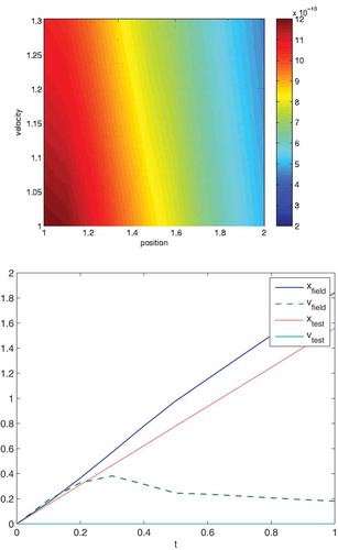
In Figure 1–2, we present the impact oscillator with $ϵ=0.1$ with the Hamiltonian schemes. We see an improvement with the additional multiscale solution instead of the pure onescale solution. The result is more precise, which can be seen with the relaxation results of $x_1$ and $v_1$.

Figure 1. We apply $U(x,0.1)=0.1\frac{1}{x^2}+x^2,E(x,0.1)=0.1\frac{2}{x^3}-2x$, where $ϵ=0.1$ and the starting points are $(x,v{)}^{\mathrm{T}}=(1.0,1.0{)}^{\mathrm{T}}$. The figure presents the contours of the impact oscillator with the multiscale solution $(x,v{)}^{\mathrm{T}}=(x_0,v_0{)}^{\mathrm{T}}+ϵ(x_1,v_1{)}^{\mathrm{T}}$. The colour bars are contour plots of the equilibrium density $\pi (x,v)$ in Equation (68).

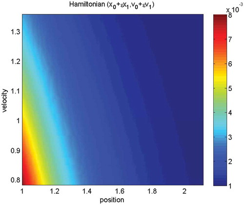
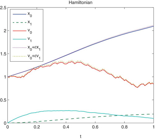
Figure 2. We apply $U(x,0.1)=0.1\frac{1}{x^2}+x^2,E(x,0.1)=0.1\frac{2}{x^3}-2x$, where $ϵ=0.1$ and the starting points are $(x,v{)}^{\mathrm{T}}=(1.0,1.0{)}^{\mathrm{T}}$. The figure presents a relaxation of the impact oscillator with $ϵ=0.1$. The labels of the $y$-axis are dimensionless quantities of the positions $x_0,x_1$ and the velocities $v_0,v_1$.

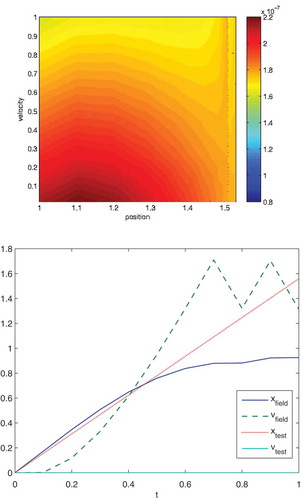
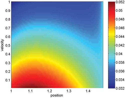
In Figure 3–4, we present the full impact oscillator, which means with $ϵ=1.0$ with the Hamiltonian schemes and the EM without multiscale approach as reference scheme.

Figure 3. We apply $U(x,1.0)=\frac{1}{x^2}+x^2,E(x,1.0)=\frac{2}{x^3}-2x$, where $ϵ=1.0$ and the starting points are $(x,v{)}^{\mathrm{T}}=(1.0,1.0{)}^{\mathrm{T}}$. The upper figure presents the contours of the impact oscillator with the multiscale solution of the Hamiltonian Splitting (multiscale solution $(x,v{)}^{\mathrm{T}}=(x_0,v_0{)}^{\mathrm{T}}+ϵ(x_1,v_1{)}^{\mathrm{T}}$). The lower figure presents a relaxation of the impact oscillator with the multiscale solution of the Hamiltonian Splitting with $ϵ=1.0$. The labels of the $y$-axis are dimensionless quantities of the positions $x_0,x_1$ and the velocities $v_0,v_1$.

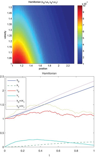
Figure 4. We apply $U(x,1.0)=\frac{1}{x^2}+x^2,E(x,1.0)=\frac{2}{x^3}-2x$, where $ϵ=1.0$ and the starting points are $(x,v{)}^{\mathrm{T}}=(1.0,1.0{)}^{\mathrm{T}}$. The upper figure presents the contours of the impact oscillator with the exact solution of the EM scheme without multiscale approach (full solution $(x,v{)}^{\mathrm{T}}$). The colour bars are contour plots of the equilibrium density $\pi (x,v)$ in Equation (68). The lower figure presents a relaxation of the impact oscillator with the exact solution of the EM scheme without multiscale approach with $ϵ=1.0$. The labels of the $y$-axis are dimensionless quantities of the positions $x$ and the velocities $v$.

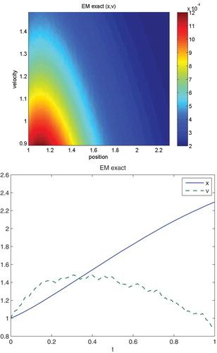
We see an improvement with the additional multiscale solution instead of the pure onescale solution. For problems with such high impacts, it is necessary to apply the full multiscale solution to control the blow-up (impact) term. Based on calculating the different multiscale equations independently, we could apply smaller time-steps for the blow-up terms, means for the $x_1$ and $v_1$ solutions. Here, we apply time-steps, which are ${10}^2-{10}^4$ times smaller,and could improved the multiscale approach. In the relaxation results of $x_1$ and $v_1$, we also see the improved behaviour of the convergence.

Remark 4.1. In the experiments, we obtain the benefit of the multiscale method, achieving more flexibility to controll the blow-up term of the models, see [42]. We obtain a relaxed phase-space problem and could also compute the delicate impact oscillator with the collision effects and controll the blow-up with the multiscale approach. This means the additional multiscale values $x_1$ and $v_1$ are important for seeing the relaxation of the position and velocity of the particles. Further the qualitative error is reduced with the multiscale approach and we could control the blow-up for impact oscillators with different $ϵ=\left\{0.1,1.0\right\}$, see Figure 1–4. Here, the combination of the multiscale approach and the splitting approach reduces both errors (qualitative and quantitative), see also [1].

In the following, we test the benefit of the multiscale approach with respect to the blow-up for $x\to 0$. We apply the error norm, which is given in Equation (64), to present the decreasing of the error with respect to $ϵ\to 0$. The exact solution, which we apply with a fine resolution of the EM scheme without multiscale approach, see Equations (51)-(52), is compared with the solutions of the EM scheme with multiscale approach, see Equations (58)-(63).

We apply the different starting points

$(x(0),v(0))=\left\{(0.001,1.0),(0.01,1.0),(0.1,1.0),(1.0,1.0)\right\}$, and the different multiscale factors $ϵ=\left\{1.0,0.1,0.01,0.001\right\}$.

In Figure 5–6, we present the blow-up error with respect to the multiscale approach.

Figure 5. Numerical blow-up errors of the EM with the multiscale approach for the $x$-version for a short time interval ($t\in [0,10]$). We compare the multiscale approach with a very fine reference solution ($\mathrm{\Delta }t/256$) of the EM without the multisplitting approach.

Figure 6. Numerical blow-up errors of the EM with the multiscale approach for the $v$-version for a short time interval ($t\in [0,10]$). We compare the multiscale approach with a very fine reference solution ($\mathrm{\Delta }t/256$) of the EM without the multisplitting approach.

Remark 4.2. The blow-up errors in Figure 5–6 show the sensitivity of the initial condition $x(0)\to 0$. Even for very small time-steps of the so called exact solution, which we have done with an EM scheme without multiscale approach, we also have large errors. When, we compare moderate $x(0)=\left\{0.1,1.0\right\}$ to the exact solution, we obtain the same accuracy for the multiscale EM scheme. The blow-up error for smaller initial conditions with $x(0)=\left\{0.001,0.01\right\}$ can be controlled with appropriate $ϵ=\left\{0.01,0.001\right\}$. The same results, we also obtain for the deterministic–stochastic and Hamiltonian splitting approaches. For more accurate results in the blow-up test-case, it is necessary to apply adaptive scheme, see [42] and [18].

In the following experiments, we test the different splitting approaches to see which splitting approach benefits the speed and which benefits the accuracy.

In Figure 7–8, we present the convergence of the different splitting methods, namely, the deterministic–stochastic and Hamiltonian splitting methods. We chose a short time interval $[0,10]$ and we $\mathrm{\Delta }t=0.1$ with $N=100$ time-points. We apply the numerical error, which is given in Equation (64).

Figure 7. Numerical errors of the deterministic–stochastic AB and ABA splittings, Hamiltonian AB, ABA ($x$-version) and ABA ($v$-version) with multiscale approach for a short time interval, where we apply a very fine reference solution (with $\mathrm{\Delta }t/256$) of the EM without multiscale approach. The figure presents the numerical errors of the position $x$. The strongest reduction of the errors for such short time intervals is given with the D/S-ABA splitting method.

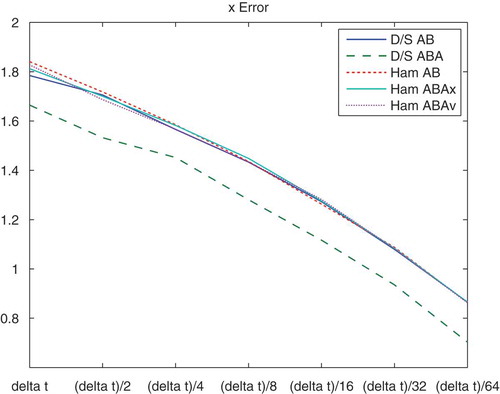
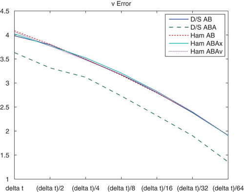
Figure 8. Numerical errors of the deterministic–stochastic AB and ABA splittings, Hamiltonian AB, ABA ($x$-version) and ABA ($v$-version) with multiscale approach for a short time interval, where we apply a very fine reference solution (with $\mathrm{\Delta }t/256$) of the EM without multiscale approach. The figure presents the numerical errors of the velocity $v$. The strongest reduction of the errors for such short time intervals is given with the D/S-ABA splitting method.

In Figure 9–10, we present the convergence of the different splitting methods. We chose a long time interval $[0,1000]$ and $\mathrm{\Delta }t=0.1$ with $N=10000$ time-points. We apply the numerical error, which is given in Equation (64). For such long time intervals, we see the benefit of the higher order splitting scheme, i.e. deterministic–stochastic and Hamiltonian splitting methods.

Figure 9. Numerical errors of the EM, deterministic–stochastic AB and ABA splittings, Hamiltonian AB, ABA ($x$-version) and ABA ($v$-version) for the long time interval with multiscale approach, where we apply a very fine reference-solution (with $\mathrm{\Delta }t/256$) of an EM without multiscale approach. The figure presents the numerical errors of the position $x$ of all methods. The strongest reduction of the errors for such long time intervals are with the Ham-ABA splitting method.

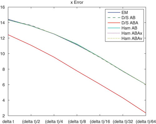
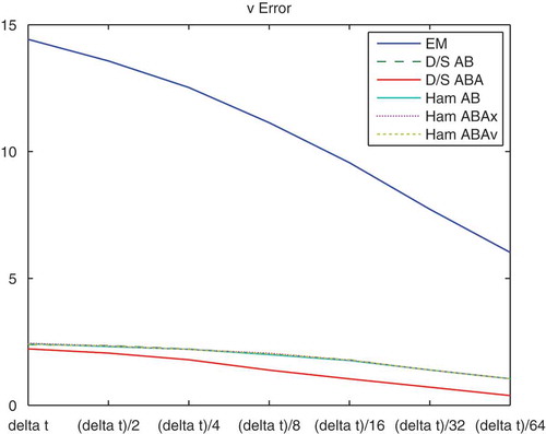
Figure 10. Numerical errors of the EM, deterministic–stochastic AB and ABA splittings, Hamiltonian AB, ABA ($x$-version) and ABA ($v$-version) for the long time interval with multiscale approach, where we apply a very fine reference-solution (with $\mathrm{\Delta }t/256$) of an EM without multiscale approach. The figure presents the numerical errors of the velocity $v$ of all methods. The strongest reduction of the errors for such long time intervals are with the Ham-ABA splitting method.

Remark 4.3. We obtain the benefit of the ABA splitting approach in both short and long time intervals. For the short and long time interval, the deterministic–stochastic ABA splitting approach is more accurate and we obtain the reduction of the errors based on the higher order accuracy. We also tested much more larger time intervals and we obtain a benefit of the Hamiltonian ABA splitting approach. Here, we see that the Hamiltonian splitting has the best accuracy of the splitting approaches for the long time intervals based on its symplecticity. But it is more expensive to compute, for we have two A-steps and one B-step. Based on its use of smaller time-steps, it obtains good accuracy. Further, we also obtain very good results with a simpler AB splitting approach, for we have one A-step and one B-step, which is faster to compute. Therefore, an optimal choice between accuracy and efficiency is in following the AB splitting approach.

Remark 4.4. For the schemes that apply the Euler–Maruyama method as a discrete solver method, we obtain an order of $\mathcal{O}(\mathrm{\Delta }{t}^{1/2})$. For schemes that apply in addition the Milstein method as a discrete solver method, we obtain an order of $\mathcal{O}(\mathrm{\Delta }t)$. The multiscale methods improve the accuracy with respect to the order of the expansion, so that we obtain one order more accuracy, which means we obtain a first-order solution with $x(t,ϵ)=x_0+ϵx_1$ instead of the zeroth order solution with $x(t,ϵ)=x_0$. Numerically, we have an improvement when we apply higher order splitting schemes, meaning the Hamiltonian-ABA or Stochastic–Deterministic-ABA splitting approaches. Here we obtain an order of $\mathcal{O}(\mathrm{\Delta }t)$ instead of the order $\mathcal{O}(\mathrm{\Delta }{t}^{1/2})$ of the classical AB splitting schemes. Such higher order approaches allow to reduce the error and we obtain smaller errors for the long time interval simulations, see also [1] and [86].

4.2. 3D example: simulation of a multi-particle model with transport and collision terms

In the following, we consider different 3D experiments related to a particle model with collisions. The modelling is based on designing plasma reactors with low temperature plasma, see [29]. Such reactors are used for the deposition of thin films on a different material, see [27] and [30]. The kinetic phenomena are crucial and important for the design of such apparatus, see [13]. We concentrate on small-angle scattering, which dominates in Coulomb collisions. Here, realistic models are given with Argon plasma, where the simulations are important for controlling the relaxation in the particle interactions, see [86]. We concentrate on collisions between ions and ions, i.e. Ar${ }^{+}$–Ar${ }^{+}$, see [4].

Particle simulation for the Coulomb collision is discussed in [87] and [60]. Here the underlying idea is to enrich a PIC code to solve models of low-density plasma interactions with a collision model, see [87] and [2].

We discuss the modelling and the algorithmic benefits for a fluid composed of Coulomb-interacting particles, see [38] and [76]. The benefit to our modelling will be the improvement with respect to the full Coulomb collision term, see the ideas in [3]. We assume that based on the electrostatic field, the plasma oscillations and their underlying molecular dynamics are of an harmonic oscillator or an impact oscillator, see [42,87] and [29].

We study the following examples:

• Two particles with reduced collision function,

• Two particles with full collision function,

• Multiple particles with full collision functions,

and for the Coulomb collision, we deal with $e-e$, $e-A^{+}$, $A^{+}-A^{+}$, where $e$ is an electron and $A^{+}$ is an ion, e.g. an Argon ion, see the deposition model in [29] and [4].

For all experiments, we employ the following parameters of the factors in the collision functions:

(69) $A_D=8\pi n_f{q}_t^2{q}_f^2\frac{ln\mathrm{\Lambda }}{m_t^2}=2.005,l_f=\sqrt{\frac{m_f}{2T_f}}\approx {10}^{-4},$(69)

where the parameters are given by

• $n_f=2{10}^{19}$ [m${ }^{-3}$] is the density of the field particles,

• $ln\mathrm{\Lambda }=10-17$ is the Coulomb logarithm (weakly coupled plasma), see [3] and [88],

• $T_f=1500$ [K] is the temperature of the field particle,

• $q_t=1.602{10}^{-19}$ [C] and $q_f=1.602{10}^{19}$ [C] are the charges of the test particle and field particle,

• $m_t=1.672{10}^{-27}$ [kg] and $m_f=1.672{10}^{-27}$ [kg] are the masses of the test particle and field particle.

These are the same parameters as were given in [3] for a many-particle experiment.

We employ the following collision functions:

(70) $F_d(v)=-\frac{A_D}{2v^2}\left[\left[4l_f^2{v}^2+1\right]G(l_{f}v)-\varphi (l_{f}v)\right],$(70)

(71) $D_v(v)=\frac{A_D}{2v}G(l_{f}v)$(71)

(72) $D_a(v)=\frac{A_D}{4v^3}\left[\varphi (l_{f}v)-G(l_{f}v)\right],$(72)

where $\varphi (x)=erf(x)$ is the error function and $G(x)=\frac{erf(x)-xer{f}^{\prime }(x)}{x}$ with $er{f}^{\prime }(x)=\frac{1}{\sqrt{\pi }}exp(-x^2)$.

In the following, we apply the experimental ideas of [2,3,37], and [14].

For such experiments, we have instationary distributions of the Langevin equation. We do not have stationary solutions and therefore it means the Gibbs distribution is not fulfilled, see [52]. For such experiments, it is sufficient to compare the qualitative behaviour of the solutions, see [3].

4.2.1. 3D example: two-particle model with transport and reduced coulomb collision term

In the following example, we treat two particles, one particle being the test particle and the other particle the field particle. We assume that one particle is not influenced by the E-field. We apply the reduced Coulomb collision term that is discussed in [14] and test the benefits of such efficient collision terms.

Further, we deal with a scaled velocity field, so that we can start with the following initialization:

(73) ${\mathbf{x}}_f=(1.0,1.0,1.0{)}^t,{\mathbf{v}}_f=(1.0,1.0,1.0{)}^t,$(73)

(74) ${\mathbf{x}}_t=(0.9,0.9,0.9{)}^t,{\mathbf{v}}_t=(0.9,0.9,0.9{)}^t.$(74)

We apply the following $E$-field:

(75) $\mathbf{E}({\mathbf{x}}_{lab}(t),ϵ)={\left({ϵ}_x\frac{2}{x_{lab}^3}-2x_{lab},{ϵ}_y\frac{2}{y_{lab}^3}-2y_{lab},{ϵ}_z\frac{2}{z_{lab}^3}-2z_{lab}\right)}^t,$(75)

where $ϵ=({ϵ}_x,{ϵ}_y,{ϵ}_z{)}^t$, ${ϵ}_x,{ϵ}_y,{ϵ}_z\in [0,1]$.

For the experiments, we choose $({ϵ}_x,{ϵ}_y,{ϵ}_z{)}^t=(0,0,0{)}^t$ for the harmonic behaviour of the 3D-oscillator. For $({ϵ}_x,{ϵ}_y,{ϵ}_z{)}^t=(1.0,1.0,1.0{)}^t$ we have an impact behaviour of the 3D-oscillator if $x_f\to (0,0,0)$.

The potential function is given by

(76) $U({\mathbf{x}}_{lab}(t),ϵ)={ϵ}_x\frac{1}{x_{lab}^2}+x_{lab}^2+{ϵ}_y\frac{1}{y_{lab}^2}+y_{lab}^2+{ϵ}_z\frac{1}{z_{lab}^2}+z_{lab}^2{)}^t$(76)

$=-\mathrm{\nabla }\cdot \mathbf{E}({\mathbf{x}}_{lab}(t),ϵ),$

and the approximate heat map is given by

(77) $\pi (\mathbf{x},\mathbf{v},ϵ)=C^{-1}exp\left(-\beta [\frac{{\mathbf{v}}^t\mathbf{v}}{2}+U(\mathbf{x},ϵ)]\right),$(77)

where $C^{-1}=1.0$ and $\beta =1.0$. For the visualization, we choose $x_x=x_y=x_z$ and $v_x=v_y=v_z$.

Algorithm 5 gives the AB splitting for the two particles.

Algorithm 5 AB splitting algorithm with multiscale approaches for coupling transport and collision of the plasma-simulation

• 1: Input: ${\mathbf{x}}_i(t^0),{\mathbf{v}}_i(t^0)$ are the spatial- and velocity-coordinates of the particles, $i=1,2$. We separate into a field particle ${\mathbf{x}}_f(t^0)={\mathbf{x}}_1(t^0)$, ${\mathbf{v}}_f(t^0)={\mathbf{v}}_1(t^0)$ and a test particle ${\mathbf{x}}_f(t^0)={\mathbf{x}}_1(t^0)$, ${\mathbf{v}}_t(t^0)={\mathbf{v}}_2(t^0)$. $t^n$, for $n=0,\dots ,\tilde{N}$, are the time-points, $t^0$ is the initial time, and $t^{\tilde{N}}$ is the ending time.

• 2: for $n=0,\dots ,\tilde{N}-1$ do

• 3: Step A ($t^n\to t^{n+1}$) (transport of the field particle):

(78) ${\tilde{\mathbf{x}}}_f(t^{n+1})={\mathbf{x}}_f(t^n)+\mathrm{\Delta }t{\mathbf{v}}_f(t^n),$(78)

(79) ${\tilde{\mathbf{v}}}_f(t^{n+1})={\mathbf{v}}_f(t^n)+\mathrm{\Delta }t\mathbf{E}({\mathbf{x}}_f(t^n),ϵ),$(79)

(transport of the test particle without being influence by the field):

(80) ${\tilde{\mathbf{x}}}_t(t^{n+1})={\mathbf{x}}_t(t^n)+\mathrm{\Delta }t{\mathbf{v}}_t(t^n),$(80)

(81) ${\tilde{\mathbf{v}}}_t(t^{n+1})={\mathbf{v}}_t(t^n).$(81)

4: Transformation into the local coordinate system:

(82) $\tilde{v}(t^{n+1})=\sqrt{v_{local,x}^2(t^{n+1})+v_{local,y}^2(t^{n+1})+v_{local,z}^2(t^{n+1})},$(82)

(83) $\tilde{\theta }(t^{n+1})=\mathrm{a}\mathrm{r}\mathrm{c}\mathrm{c}\mathrm{o}\mathrm{s}\left(\frac{v_{local,z}(t^{n+1})}{\tilde{v}(t^{n+1})}\right),$(83)

(84) $\tilde{\varphi }(t^{n+1})=\mathrm{a}\mathrm{r}\mathrm{c}\mathrm{t}\mathrm{a}\mathrm{n}\left(\frac{v_{local,y}(t^{n+1})}{v_{local,x}(t^{n+1})}\right),$(84)

where ${\mathbf{v}}_{local}(t^{n+1})={\tilde{\mathbf{v}}}_t(t^{n+1})-{\tilde{\mathbf{v}}}_f(t^{n+1})$.

5: Step B (Collision of the field and test particles in the local coordinate system):

(85) $v(t^{n+1})=\tilde{v}(t^{n+1})-\beta (\tilde{v}(t^{n+1}))\tilde{v}(t^{n+1}))\mathrm{\Delta }t+\sqrt{{\delta }^2(\tilde{v}(t^{n+1}))}\mathrm{\Delta }{W}_v,$(85)

(86) $\theta (t^{n+1})=\tilde{\theta }(t^{n+1})+\sqrt{2\gamma (\tilde{v}(t^{n+1}))}\mathrm{\Delta }{W}_{\theta },$(86)

(87) $\varphi (t^{n+1})=\tilde{\varphi }(t^{n+1})+2\pi U_{\varphi }(0,1),$(87)

where we apply the following reduced collision functions with $0<v<<1$, see [14]. The reduced collision functions are related to the collision functions defined in Equations (70)–(72):

(88) $2D_a(v)\approx \gamma (v)=\frac{2}{3\sqrt{\pi }}{A}_D\frac{l_f}{v^2},$(88)

$-F_d(v)\approx \beta (v)v=-\frac{1}{\sqrt{\pi }}{A}_D\frac{l_f}{v^2}v,$

(89) $2D_v(v)\approx {\delta }^2(v)=\frac{2}{3\sqrt{\pi }}{A}_D{l}_f.$(89)

Further, we have $\mathrm{\Delta }t=t_{n+1}-t_n$, $\mathrm{\Delta }{W}_i=W_{i,t_{n+1}}-W_{i,t_n}=\sqrt{\mathrm{\Delta }t}{\xi }_i$, where $⟨{\xi }_i⟩=0$ and $⟨{\xi }_i^2⟩=1$ with $i=\left\{v,\theta \right\}$ being two independent normally distributed random variables. Further, $U_{\varphi }(0,1)$ is a temporally uncorrelated uniform random variable between $[0,1]$. The critical CFL condition is related to the collision Equation (85) and given by

(90) $\mathrm{\Delta }t\le \frac{1}{|\tilde{v}(t^{n+1})|},$(90)

where we assume $\beta (\tilde{v}(t^{n+1}))\approx -\frac{F_d(\tilde{v}(t^{n+1}))}{\tilde{v}(t^{n+1})}\approx \frac{1}{\tilde{v}(t^{n+1})}$.

Further, for sufficiently small $v\to 0$, we omit the stochastic term in (85), see [14], and apply only the deterministic equation:

(91) $v(t^{n+1})=\sqrt{{\tilde{v}}^2(t^{n+1})+\frac{4}{3\sqrt{\pi }}{A}_D{l}_f\mathrm{\Delta }t}.$(91)

6: Transformation step: Local to common coordinate system

We have to shift the velocity back into the common coordinate system:

(92) ${\mathbf{v}}_f(t^{n+1})={\tilde{\mathbf{v}}}_f(t^{n+1})+{\epsilon }_{coll}$(92)

$\cdot \left(\begin{array}{ccc}cos(\tilde{\theta }(t^{n+1}))cos(\tilde{\varphi }(t^{n+1}))& -sin(\tilde{\varphi }(t^{n+1}))& sin(\tilde{\theta }(t^{n+1}))cos(\tilde{\varphi }(t^{n+1}))\\ cos(\tilde{\theta }(t^{n+1}))sin(\tilde{\varphi }(t^{n+1}))& cos(\tilde{\varphi }(t^{n+1}))& sin(\tilde{\theta }(t^{n+1}))sin(\tilde{\varphi }(t^{n+1}))\\ -sin(\tilde{\theta }(t^{n+1}))& 0& cos(\tilde{\varphi }(t^{n+1}))\\ \hspace{0.17em}& \hspace{0.17em}& \hspace{0.17em}\end{array}\right).$

$\cdot \left(\begin{array}{c}\left[\tilde{v}(t^{n+1})+\mathrm{\Delta }v\right]sin(\mathrm{\Delta }\theta )cos(\mathrm{\Delta }\varphi )\\ \left[\tilde{v}(t^{n+1})+\mathrm{\Delta }v\right]sin(\mathrm{\Delta }\theta )sin(\mathrm{\Delta }\varphi )\\ \left[\tilde{v}(t^{n+1})+\mathrm{\Delta }v\right]cos(\mathrm{\Delta }\varphi )\\ \hspace{0.17em}\end{array}\right)$

where $\mathrm{\Delta }\varphi =\varphi (t^{n+1})-\tilde{\varphi }(t^{n+1})$, $\mathrm{\Delta }\theta =\theta (t^{n+1})-\tilde{\theta }(t^{n+1})$, $\mathrm{\Delta }v=v(t^{n+1})-\tilde{v}(t^{n+1})$, where we have an additional ${ϵ}_{coll}\in [0,1]$ factor to test the influence of the collision.

For ${ϵ}_{coll}=0$, we omit the collision term, whereas for ${ϵ}_{coll}=1$, we have the full collision term. Such a parameter is used to make perceptible the collision.

(93) ${\mathbf{x}}_f(t^{n+1})={\tilde{\mathbf{x}}}_f(t^{n+1}),{\mathbf{x}}_t(t^{n+1})={\tilde{\mathbf{x}}}_t(t^{n+1}),$(93)

(94) ${\mathbf{v}}_f(t^{n+1})={\tilde{\mathbf{v}}}_f(t^{n+1}),{\mathbf{v}}_t(t^{n+1})={\tilde{\mathbf{v}}}_t(t^{n+1}).$(94)

7: end for

8: The output is given by ${\mathbf{x}}_1(t^n)={\mathbf{x}}_f(t^n),{\mathbf{v}}_1(t^n)={\mathbf{v}}_f(t^n),{\mathbf{x}}_2(t^n)={\mathbf{x}}_t(t^n){\mathbf{v}}_2(t^n)={\mathbf{v}}_t(t^n)$ are the spatial- and velocity-coordinates of the particles with $i=1,2$ and $n=1\dots ,\tilde{N}$.

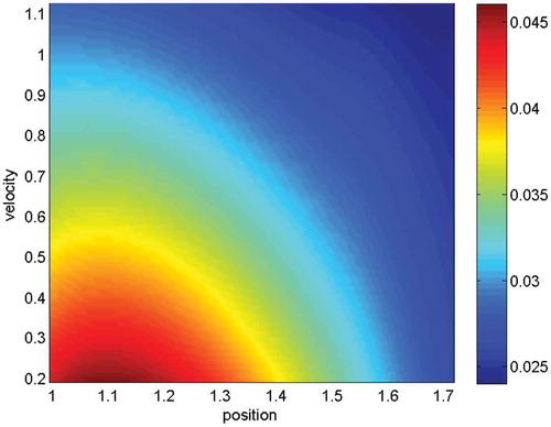
In Figure 11–12, we present the 3D impact oscillator of the reduced model with ${ϵ}_x={ϵ}_y={ϵ}_z=1.0$ and the collision term with ${ϵ}_{coll}=1.0$.

Figure 11. The heat maps are computed with respect to the different slices in $x$, $y$ and $z$ direction. In the upper figure, the solutions are given with $(x_x,0,0,v_x,0,0,1.0)$ ($x$-slice). In the lower figure, the solutions are given with $(0,x_y,0,0,v_y,0,1.0)$ ($y$-slice). The colour bars are contour plots of the equilibrium density $\pi (x,v)$ in Equation (77). We see homogeneous heat maps for all three coordinates, which means we have a stable simulation, see [42].

Figure 12. The heat maps are computed with respect to the different slices in $x$, $y$ and $z$ direction. In figure, the solutions are given with $(0,0,x_z,0,0,v_z,1.0)$ ($z$-slice). The colour bars are contour plots of the equilibrium density $\pi (x,v)$ in Equation (77). We see homogeneous heat maps for all three coordinates, which means we have a stable simulation, see [42].

Another presentation of the $6$-dimensional phase-space results can be given with the the heat map of the absolute values:

(95) $\pi (\left|\mathbf{x}\left|,\right|\mathbf{v}\right|,ϵ)=C^{-1}exp\left(-\beta \left[\frac{|\mathbf{v}{|}^2}{2}+U(\left|\mathbf{x}\right|,ϵ)\right]\right),$(95)

where $\left|\mathbf{X}\right|=\sqrt{x_x^2+x_y^2+x_z^2}$ and $\left|\mathbf{v}\right|=\sqrt{v_x^2+v_y^2+v_z^2}\mathrm{a}\mathrm{n}\mathrm{d}U(\left|\mathbf{x}\right|,ϵ)={ϵ}_x\frac{1}{x_{lab}^2}+x_{lab}^2+{ϵ}_y\frac{1}{y_{lab}^2}+y_{lab}^2+{ϵ}_z\frac{1}{z_{lab}^2}+z_{lab}^2{)}^t$, for ${\epsilon }_x={\epsilon }_y={\epsilon }_z$.

In Figure 13, we present the 3D impact oscillator of the reduced model and the relaxation time to achieve a stable numerical solution with ${ϵ}_x={ϵ}_y={ϵ}_z=1.0$ and the collision term with ${ϵ}_{coll}=1.0$.

Figure 13. In the upper figure, the heat map is computed with respect to the absolute values of the phase-space coordinates, i.e. $\left|\mathbf{x}\right|=\sqrt{x_x^2+x_y^2+x_z^2}$ and $\left|\mathbf{v}\right|=\sqrt{v_x^2+v_y^2+v_z^2}$. The colour bars are contour plots of the density $\pi (x,v)$ in Equation (95). We obtain an homogeneous heatmap, which our numerical schemes.

In the lower figure, we apply the amplitudes of the field and test particles around the averaged value, which are given by $x_a=\sqrt{{(x_{a,x}(0)-x_{a,x}(t))}^2+{(x_{a,y}(0)-x_{a,y}(t))}^2+{(x_{a,z}(0)-x_{a,z}(t))}^2}$ and $v_a=\sqrt{{(v_{a,x}(0)-v_{a,x}(t))}^2+{(v_{a,y}(0)-v_{a,y}(t))}^2+{(v_{a,z}(0)-v_{a,z}(t))}^2}$ with $a=\left\{field,test\right\}$. The labels of the $y$-axis are dimensionless quantities of the positions $x_{field},x_{test}$ and the velocities $v_{field},v_{test}$. Based on the homogeneous heatmap, we obtain a linear behaviour in the $x$-direction and a constant behaviour in the $v$-direction.

Remark 4.5. We obtain a relaxation in the velocities of the test and field particle, so that we could stabilize the interactions in the particle collisions. Based on the time-step restrictions in the numerical schemes, we also obtain homogeneous heat maps; such qualitative information of the non-linear dynamics allows stable simulations, see [42]. Further, we obtain the benefit of splitting methods and could achieve relaxed solutions. The multiscale method allows applying the reduced model without damping the collision part (${\epsilon }_{coll}=1.0$). In each coordinate, we obtain a relaxed phase-space problem and stabilize the delicate impact oscillator with the collision effects.

4.2.2. 3D example: two-particle model with transport and full coulomb collision term

In the following, we deal with the two-particle model and the transport and Coulomb collision terms. Here, we apply the full collision functions, which are given in Equations (70)–(72). The full Coulomb collision term is discussed in [2] and [3].

We have the same initialization as in the previous test case and apply the following Algorithm 6.

Algorithm 6 AB splitting algorithm with multiscale approaches in the discretised version (explicit Euler- and Euler–Maruyama scheme

• 1: Input: ${\mathbf{x}}_i(t^0),{\mathbf{v}}_i(t^0)$ are the spatial- and velocity-coordinates of the particles, $i=1,2$. We separate into a field particle ${\mathbf{x}}_f(t^0)={\mathbf{x}}_1(t^0)$, ${\mathbf{v}}_f(t^0)={\mathbf{v}}_1(t^0)$ and a test particle ${\mathbf{x}}_f(t^0)={\mathbf{x}}_1(t^0)$, ${\mathbf{v}}_t(t^0)={\mathbf{v}}_2(t^0)$. $t^n$, for $n=0,\dots ,\tilde{N}$, are the time-points, $t^0$ is the initial time, and $t^{\tilde{N}}$ is the ending time.

• 2: for $n=0,\dots ,\tilde{N}-1$ do

• 3: Step A is as in Algorithm 5

Further, we make the transformation $\tilde{\mu }(t^{n+1})=cos(\tilde{\theta }(t^{n+1}))$.

• 4:

• 5: Step B (Collision of the field and test particles in the local coordinate system):

(96) $v(t^{n+1})=\left\{\begin{array}{cc}\sqrt{{\tilde{v}}^2(t^{n+1})+\frac{4}{3\sqrt{\pi }}{A}_D{l}_f\mathrm{\Delta }t}& \tilde{v}(t^{n+1})\le 1.0,\\ \tilde{v}(t^{n+1})+F_d(\tilde{v}(t^{n+1}))\mathrm{\Delta }t+\sqrt{2D_v(\tilde{v}(t^{n+1}))}\mathrm{\Delta }{W}_v,& \tilde{v}(t^{n+1})\ge 1.0,\end{array}\right.$(96)

(97) $\mu (t^{n+1})=\tilde{\mu }(t^{n+1})-2D_a(\tilde{v}(t^{n+1}))\tilde{\mu }(t^{n+1})\mathrm{\Delta }t+\sqrt{2D_a(\tilde{v}(t^{n+1}))(1-\tilde{\mu }{(t^{n+1})}^2)}\mathrm{\Delta }{W}_{\mu },$(97)

(98) $\varphi (t^{n+1})=\tilde{\varphi }(t^{n+1})+\sqrt{\frac{2D_a(\tilde{v}(t^{n+1}))}{(1-\tilde{\mu }{(t^{n+1})}^2)}}\mathrm{\Delta }{W}_{\varphi },$(98)

with $\mathrm{\Delta }t=t_{n+1}-t_n$, $\mathrm{\Delta }{W}_i=W_{i,t_{n+1}}-W_{i,t_n}=\sqrt{\mathrm{\Delta }t}{N}_i(0,1)$, where $N_i(0,1)=rand$, $i=\left\{v,\mu ,\varphi \right\}$ three independent normally distributed random variables.

Further, for sufficiently small $v\to 0$, we omit the stochastic term in (85)-(87), see [14], and apply only the deterministic equation

(99) $v(t^{n+1})=\sqrt{{\tilde{v}}^2(t^{n+1})+\frac{4}{3\sqrt{\pi }}{A}_D{l}_f\mathrm{\Delta }t}.$(99)

6: Further, we make the transformation $\theta (t^{n+1})=\mathrm{a}\mathrm{r}\mathrm{c}\mathrm{c}\mathrm{o}\mathrm{s}(\mu (t^{n+1}))$.

7: Transformation step: Local to common coordinate system, as in Algorithm 5.

8: end for

9: The output is given by ${\mathbf{x}}_1(t^n)={\mathbf{x}}_f(t^n),{\mathbf{v}}_1(t^n)={\mathbf{v}}_f(t^n)$, ${\mathbf{x}}_2(t^n)={\mathbf{x}}_t(t^n),{\mathbf{v}}_2(t^n)={\mathbf{v}}_t(t^n)$ are the spatial- and velocity-coordinates of the particles with $i=1,2$ and $n=1\dots ,\tilde{N}$.

In the numerical experiments, we see a blow-up for small $v$. Therefore, we improve the model based on the following approaches to $F_d$:

(100) $F_d(v)=\left\{\begin{array}{cc}\frac{1}{\sqrt{\pi }}{A}_D\frac{l_f}{v},& \mathrm{R}\mathrm{e}\mathrm{d}\mathrm{u}\mathrm{c}\mathrm{e}\mathrm{d}\mathrm{t}\mathrm{e}\mathrm{r}\mathrm{m}:\mathrm{I}\mathrm{n}\mathrm{i}\mathrm{t}\mathrm{i}\mathrm{a}\mathrm{l}\mathrm{p}\mathrm{h}\mathrm{a}\mathrm{s}\mathrm{e}\\ \hspace{0.17em}& \mathrm{w}\mathrm{i}\mathrm{t}\mathrm{h}t\in [0,0.2],\\ \frac{1}{\sqrt{\pi }}{A}_D(\frac{l_f}{v}-\frac{2l_f}{3}-\frac{l_{f}v}{2}),& \mathrm{E}\mathrm{x}\mathrm{t}\mathrm{e}\mathrm{n}\mathrm{d}\mathrm{e}\mathrm{d}\mathrm{t}\mathrm{e}\mathrm{r}\mathrm{m}:\mathrm{T}\mathrm{r}\mathrm{a}\mathrm{n}\mathrm{s}\mathrm{i}\mathrm{t}\mathrm{i}\mathrm{o}\mathrm{n}\\ \hspace{0.17em}& \mathrm{p}\mathrm{h}\mathrm{a}\mathrm{s}\mathrm{e}\mathrm{w}\mathrm{i}\mathrm{t}\mathrm{h}t\in [0.2,0.8],\\ -\frac{A_D}{2v^2}\cdot & \mathrm{F}\mathrm{u}\mathrm{l}\mathrm{l}\mathrm{t}\mathrm{e}\mathrm{r}\mathrm{m}:\mathrm{S}\mathrm{t}\mathrm{a}\mathrm{b}\mathrm{l}\mathrm{e}\mathrm{p}\mathrm{h}\mathrm{a}\mathrm{s}\mathrm{e}\\ \cdot ([4l_f^2{v}^2+1]G(l_{f}v)-\varphi (l_{f}v)),& \mathrm{w}\mathrm{i}\mathrm{t}\mathrm{h}t\le \mathrm{0.8.}\end{array}\right.$(100)

In the following figures, we present the heat map and the oscillations around the initial values. In Figure 14–15, we present the 3D impact oscillator with ${ϵ}_x={ϵ}_y={ϵ}_z=1.0$ and the collision term with ${ϵ}_{coll}=0.01$.

Figure 14. The heat maps are computed with respect to the different slices in $x$, $y$ and $z$ direction. In the upper figure, the solutions are given with $(x_x,0,0,v_x,0,0,1.0)$ ($x$-slice). In the lower figure, the solutions are given with $(0,x_y,0,0,v_y,0,1.0)$ ($y$-slice). The colour bars are contour plots of the density $\pi (x,v)$ in Equation (77). We see homogeneous heat maps for all the coordinates, which means we have a stable simulation, see [42].

Figure 15. The heat map is computed with respect to the different slices in $x$, $y$ and $z$ direction. In the figure, the solutions are given with $(0,0,x_z,0,0,v_z,1.0)$ ($z$-slice). The colour bars are contour plots of the density $\pi (x,v)$ in Equation (77). We see a homogeneous heat map for the coordinates, which means we have a stable simulation, see [42].

In Figure 16, we present the 3D impact oscillator of the full model and the relaxation time to achieve a stable numerical solution with ${ϵ}_x={ϵ}_y={ϵ}_z=1.0$ and the collision term with ${ϵ}_{coll}=0.01$. Here, we obtained a faster relaxation with the novel splitting method.

Figure 16. In the upper figure, the heat maps are given with respect to the absolute values of the phase-space coordinates, namely, $\left|\mathbf{x}\right|=\sqrt{x_x^2+x_y^2+x_z^2}$ and $\left|\mathbf{v}\right|=\sqrt{v_x^2+v_y^2+v_z^2}$. The colour bars are contour plots of the density $\pi (x,v)$ in Equation (95). We obtain an homogeneous heatmap, which our numerical schemes.

In the lower figure, we compute the amplitudes of the field and test particles around the averaged value, which are given by $x_a=\sqrt{{(x_{a,x}(0)-x_{a,x}(t))}^2+{(x_{a,y}(0)-x_{a,y}(t))}^2+{(x_{a,z}(0)-x_{a,z}(t))}^2}$ and $v_a=\sqrt{{(v_{a,x}(0)-v_{a,x}(t))}^2+{(v_{a,y}(0)-v_{a,y}(t))}^2+{(v_{a,z}(0)-v_{a,z}(t))}^2}$ with $a=\left\{field,test\right\}$. The labels of the $y$-axis are dimensionless quantities of the positions $x_{field},x_{test}$ and the velocities $v_{field},v_{test}$. Based on the homogeneous heatmap, we obtain a linear behaviour in the $x$-direction and a constant behaviour in the $v$-direction.

Remark 4.6. We obtain the benefit of the full Coulomb collision term and we have more detailed heat maps for the different coordinates. Qualitatively an improved collision function is important to resolve the different phases, namely, the initial, transitional, and stable phases. A generalised reduced collision function, as presented in [14] is too delicate. Based on the improvements of the more detailed collision function developed, we also obtain improved relaxations in the velocities of the test and field particles. Moreover, the detailed collision functions are scale dependent and it is necessary to apply multiscale methods for the full model. The multiscale and splitting approaches resolve the relaxation of the delicate non-linear and blow-up functions. Further, if we damp the collision with ${ϵ}_{coll}=0.01$, we can obtain similar results as for the reduced model. Based on an extension with the detailed collision function and with a damped collision factor, we can solve the phase-space problem and can also compute the delicate impact oscillator with the collision effects.

4.3. 3D example: simulation of a multiple particle model related to the langevin equation

In the following, we treat a multiple particle test example, which is applied to an Argon plasma, see [86]. Such plasmas are used in deposition processes for CVD (chemical vapour deposition) and PVD (physical vapour deposition) apparatus, see [89] and [83]. The simulations are based on the transport and collision steps to the ionised particles. The results of the simulations are the relaxation of the positions and velocitites of the particles. Such results are important to foresee the stability in the particle transport to control the deposition process, see [83].

In the experiments, we use $N=100$ particles, which are Ar${ }^{+}$ ions. For the transport step, the particles are globally transported by the Newtonian transport equation and controlled by an external electrical field. For the collision step, the particles interact locally by Coulomb collisions. In the collision step, we choose each particle of the 100 particles as a test particle and use the average of the other particles as the field particle.

All particles are influenced by the electric field and we assume that we have permanent collisions of the particles. Further, we have the collision functions with the drag force and diffusion coefficients in Equations (70)–(72).

We deal with the average field particle, which is given in the common coordinate system:

(101) ${\mathbf{v}}_f=\frac{{\sum }_{j=1,j\ne \tilde{i}}^N{\mathbf{v}}_j}{N},$(101)

where ${\mathbf{v}}_{\tilde{i}}$ is the velocity of the test particle and we assume there are 100 particles.

We use the following initial conditions for all particles, where we assume the spatial steps and velocity steps of $0.01$ to the next particle. We initialize the phase-space coordinates between $[0,1]$ with

(102) ${\mathbf{x}}_1=(1.5,1.5,1.5{)}^t,{\mathbf{v}}_1=(1.5,1.5,1.5{)}^t,$(102)

(103) ${\mathbf{x}}_2=(1.49,1.49,1.49{)}^t,{\mathbf{v}}_2=(1.49,1.49,1.49{)}^t,$(103)

$⋮$

(104) ${\mathbf{x}}_{100}=(0.5,0.5,0.5{)}^t,{\mathbf{v}}_{100}=(0.5,0.5,0.5{)}^t,$(104)

where we assume a scaled velocity.

The multiscale $E$-field is given by

(105) $\mathbf{E}({\mathbf{x}}_{lab}(t),ϵ)=({ϵ}_x\frac{2}{x_{lab}^3}-2x_{lab},{ϵ}_y\frac{2}{y_{lab}^3}-2y_{lab},{ϵ}_z\frac{2}{z_{lab}^3}-2z_{lab}{)}^t,$(105)

where $ϵ=({ϵ}_x,{ϵ}_y,{ϵ}_z{)}^t$, ${ϵ}_x,{ϵ}_y,{ϵ}_z\in [0,1]$.

For the experiments, we chose $({ϵ}_x,{ϵ}_y,{ϵ}_z{)}^t=(0,0,0{)}^t$ for the harmonic behaviour of the 3D-oscillator. For $({ϵ}_x,{ϵ}_y,{ϵ}_z{)}^t=(1.0,1.0,1.0{)}^t$ we have an impact behaviour of the 3D-oscillator if ${\mathbf{x}}_f\to (0,0,0)$.

We apply the AB splitting approach, which is an optimal choice for sufficient accuracy and important computational efficiency, see also subsection 4.1. The algorithm 7 is given for the $N$-particle transport–collision simulations.

Algorithm 7 The AB splitting with multiscale approach written as an MPC Algorithm

• 1: Input: ${\mathrm{x}}_i(t^0),{\mathrm{v}}_i(t^0)$ are the spatial- and velocity-coordinates of the particles, $i=1,\dots ,N$, where $N=100$ is the number of particles. $t^n$, for $n=0,\dots ,\tilde{N}$, are the time-points, $t^0$ is the initial time, and $t^{\tilde{N}}$ is the ending time.

• 2: for $n=0,\dots ,\tilde{N}-1$ do

• 3: Step A ($t^n\to t^{n+1}$) (transport of all the particles in the common coordinate system):

(106) ${\tilde{\mathbf{x}}}_1(t^{n+1})={\mathbf{x}}_1(t^n)+\mathrm{\Delta }t{\mathbf{v}}_1(t^n),$(106)

(107) ${\tilde{\mathbf{v}}}_1(t^{n+1})={\mathbf{v}}_1(t^n)+\mathrm{\Delta }t\mathbf{E}({\mathbf{x}}_1(t^n),ϵ),$(107)

(108) $⋮$(108)

(109) ${\tilde{\mathbf{x}}}_{100}(t^{n+1})={\mathbf{x}}_{100}(t^n)+\mathrm{\Delta }t{\mathbf{v}}_{100}(t^n),$(109)

(110) ${\tilde{\mathbf{v}}}_{100}(t^{n+1})={\mathbf{v}}_{100}(t^n)+\mathrm{\Delta }t\mathbf{E}({\mathbf{x}}_{100}(t^n),\epsilon ),$(110)

• 4: for $\tilde{i}=1,\dots ,N$ do

• 5: Step A2 (test particle and field particle):

The test particle is given by ${\tilde{\mathbf{v}}}_t={\tilde{\mathbf{v}}}_i$.

The average field particle is given in the common coordinate system by

(111) ${\tilde{\mathbf{v}}}_f=\frac{{\sum }_{j=1,j\ne i}^N{\tilde{\mathbf{v}}}_j}{N-1},$(111)

which is the velocity of the field particle, assuming there are $100$ particles.

6: Transformation step: Common to local coordinate system:

(112) $\tilde{v}(t^{n+1})=\sqrt{v_{local,x}^2(t^{n+1})+v_{local,y}^2(t^{n+1})+v_{local,z}^2(t^{n+1})},$(112)

(113) $\tilde{\theta }(t^{n+1})=\mathrm{a}\mathrm{r}\mathrm{c}\mathrm{c}\mathrm{o}\mathrm{s}\left(\frac{v_{local,z}(t^{n+1})}{\tilde{v}(t^{n+1})}\right),$(113)

(114) $\tilde{\varphi }(t^{n+1})=\mathrm{a}\mathrm{r}\mathrm{c}\mathrm{t}\mathrm{a}\mathrm{n}\left(\frac{v_{local,y}(t^{n+1})}{v_{local,x}(t^{n+1})}\right),$(114)

where ${\mathbf{v}}_{local}(t^{n+1})={\tilde{\mathbf{v}}}_t(t^{n+1})-{\tilde{\mathbf{v}}}_f(t^{n+1})$ and we carry out the transformation $\tilde{\mu }(t^{n+1})=cos(\tilde{\theta }(t^{n+1}))$.

7: Step B (Collision of the field and test particles in the local coordinate system):

(115) $v(t^{n+1})=\tilde{v}(t^{n+1})+F_d(\tilde{v}(t^{n+1}))\mathrm{\Delta }t+\sqrt{2D_v(\tilde{v}(t^{n+1}))}\mathrm{\Delta }{W}_v,$(115)

$\mu (t^{n+1})=\tilde{\mu }(t^{n+1})-2D_a(\tilde{v}(t^{n+1}))\tilde{\mu }(t^{n+1})\mathrm{\Delta }t$

(116) $+\sqrt{2D_a(\tilde{v}(t^{n+1}))[1-\tilde{\mu }{(t^{n+1})}^2]}\mathrm{\Delta }{W}_{\mu },$(116)

(117) $\varphi (t^{n+1})=\tilde{\varphi }(t^{n+1})+\sqrt{\frac{2D_a(\tilde{v}(t^{n+1}))}{[1-\tilde{\mu }{(t^{n+1})}^2]}}\mathrm{\Delta }{W}_{\varphi },$(117)

with $\mathrm{\Delta }t=t_{n+1}-t_n$, $\mathrm{\Delta }{W}_i=W_{i,t_{n+1}}-W_{i,t_n}=\sqrt{\mathrm{\Delta }t}{N}_i(0,1)$, where $N_i(0,1)=rand$, $i=\left\{v,\mu ,\varphi \right\}$ being three independent normally distributed random variables. Further, make the transformation $\theta (t^{n+1})=\mathrm{a}\mathrm{r}\mathrm{c}\mathrm{c}\mathrm{o}\mathrm{s}(\mu (t^{n+1}))$.

8: Transformation step: Local to common coordinate system

We have to shift the velocity of the test particle back into the common coordinate system, which is given by

(118) $\mathbf{v}(t^{n+1})={\tilde{\mathbf{v}}}_f(t^{n+1})+{\epsilon }_{coll}\cdot$(118)

$\cdot \left(\begin{array}{ccc}cos(\tilde{\theta }(t^{n+1}))cos(\tilde{\varphi }(t^{n+1}))& -sin(\tilde{\varphi }(t^{n+1}))& sin(\tilde{\theta }(t^{n+1}))cos(\tilde{\varphi }(t^{n+1}))\\ cos(\tilde{\theta }(t^{n+1}))sin(\tilde{\varphi }(t^{n+1}))& cos(\tilde{\varphi }(t^{n+1}))& sin(\tilde{\theta }(t^{n+1}))sin(\tilde{\varphi }(t^{n+1}))\\ -sin(\tilde{\theta }(t^{n+1}))& 0& cos(\tilde{\varphi }(t^{n+1}))\\ \hspace{0.17em}& \hspace{0.17em}& \hspace{0.17em}\end{array}\right)\cdot$

$\cdot \left(\begin{array}{c}\tilde{v}(t^{n+1})sin(\mathrm{\Delta }\theta )cos(\mathrm{\Delta }\varphi )\\ \tilde{v}(t^{n+1})sin(\mathrm{\Delta }\theta )sin(\mathrm{\Delta }\varphi )\\ \tilde{v}(t^{n+1})cos(\mathrm{\Delta }\varphi )\\ \hspace{0.17em}\end{array}\right),$

where $\mathrm{\Delta }\varphi =\varphi (t^{n+1})-\tilde{\varphi }(t^{n+1})$, $\mathrm{\Delta }\theta =\theta (t^{n+1})-\tilde{\theta }(t^{n+1})$,

9: $\mathrm{\Delta }{\mathbf{v}}_i(t^{n+1})=\mathbf{v}(t^{n+1})-{\tilde{\mathbf{v}}}_f(t^{n+1})$, where we have an additional ${ϵ}_{coll}\in [0,1]$ factor to test the influence of the collision.

For ${ϵ}_{coll}=0$, we omit the collision term, whereas for ${\epsilon }_{coll}=1$, we have the full collision term.

At the end of all the collisions, we have to update the locations in phase-space of all the particles.

(119) ${\mathbf{x}}_i(t^{n+1})={\tilde{\mathbf{x}}}_i(t^{n+1}),$(119)

(120) ${\mathbf{v}}_i(t^{n+1})={\tilde{\mathbf{v}}}_i(t^{n+1})+\mathrm{\Delta }{\mathbf{v}}_i.$(120)

• 10: end for

• 11: end for

• 12: The output is given by ${\mathbf{x}}_i(t^n),{\mathbf{v}}_i(t^n)$, the spatial- and velocity-coordinates of the particles with $i=1,\dots ,N$ and $n=1\dots ,\tilde{N}$.

In Figure 17–18, we present the 3D impact oscillator with ${ϵ}_x={ϵ}_y={ϵ}_z=1.0$ and the collision term with ${ϵ}_{coll}=1.0$. We apply the mean values of the position and the velocities.

Figure 17. The heatmaps are given with respect to the different coordinate-slices. We compare the mean-value for all the particles $(N=100)$ and apply the full Coulomb collision model. In the upper figure, the solutions are given with $(x_x,0,0,v_x,0,0,1.0)$ ($x$-slice). In the lower figure, the solutions are given with $(0,x_y,0,0,v_y,0,1.0)$ ($y$-slice). The color bars are contour plots of the density $\pi (x,v)$ in Equation (77). The heatmaps are homogeneous and therefore we have stable numerical schemes. We also obtain an oscillatory behaviour based on strong collisions with the particles. Such a behaviour is seen with oscillations in the heatmaps; such oscillations can be reduced with smaller ${ϵ}_{coll}$.

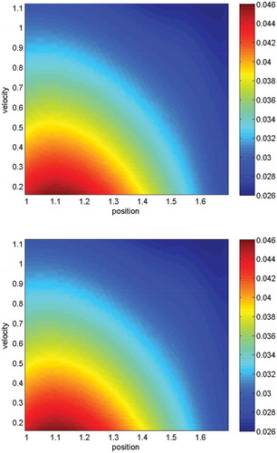
Figure 18. The heatmap is given with respect to the different coordinate-slices. We compare the mean-value for all the particles $(N=100)$ and apply the full Coulomb collision model. In the figure, the solutions are given with $(0,0,x_z,0,0,v_z,1.0)$ ($z$-slice). The color bars are contour plots of the density $\pi (x,v)$ in Equation (77). The heatmap is homogeneous and therefore we have stable numerical schemes. We also obtain an oscillatory behaviour based on strong collisions with the particles. Such a behaviour is seen with oscillations in the heatmaps; such oscillations can be reduced with smaller ${ϵ}_{coll}$.

In Figure 19–20, we present the 3D impact oscillator with ${ϵ}_x={ϵ}_y={ϵ}_z=1.0$ and the collision term with ${ϵ}_{coll}=1.0$. We apply the value of the position and the velocity of particle $i=50$.

Figure 19. The heatmaps are given with respect to the different slices in $x$, $y$ and $z$ direction. We compare the values of particle $i=50$ and apply the full Coulomb collision model. In the upper figure, the solutions are given with $(x_x,0,0,v_x,0,0,1.0)$ ($x$-slice). In lower figure, the solutions are given with $(0,x_y,0,0,v_y,0,1.0)$ ($y$-slice). The color bars are contour plots of the density $\pi (x,v)$ in Equation (77). Based on the oscillatory behaviour of the collisions, we also obtain oscillations in the heatmaps; such oscillations can be reduced with smaller ${ϵ}_{coll}$.

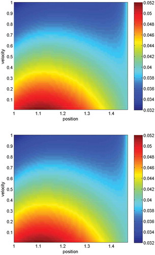
Figure 20. The heatmap is given with respect to the different slices in $x$, $y$ and $z$ direction. We compare the values of particle $i=50$ and apply the full Coulomb collision model. In the figure, the solutions are given with $(0,0,x_z,0,0,v_z,1.0)$ ($z$-slice). The color bars are contour plots of the density $\pi (x,v)$ in Equation (77). Based on the oscillatory behaviour of the collisions, we also obtain oscillations in the heatmap; such oscillations can be reduced with smaller ${ϵ}_{coll}$.

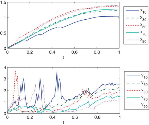
For the mean values over all particle positions and velocities, we obtain a more relaxed heatmap. We can relax single oscillatory particle results, such that the averaged particles can result into stable formations for the underlying local collision cells, see [3] and [14].

The relaxation time to achieve a stable solution is given in Figure 21. The phase-space solution stabilised to $x_i=[1.0,1.5]$ and $v_i=[1,3]$, with $i=1,\dots ,100$. With the novel splitting approach, we obtained a faster relaxation and a stable solution.

Figure 21. We present the oscillations of phase-space coordinates of single particles around the phase-space coordinates of averaged particle, which are given by $x_i=\sqrt{{(x_{i,x}(0)-x_{i,x}(t))}^2+{(x_{i,y}(0)-x_{i,y}(t))}^2+{(x_{i,z}(0)-x_{i,z}(t))}^2}$ and $v_i=\sqrt{{(v_{i,x}(0)-v_{i,x}(t))}^2+{(v_{i,y}(0)-v_{i,y}(t))}^2+{(v_{i,z}(0)-v_{i,z}(t))}^2}$ with $i=\left\{10,30,50,70,90\right\}$. The upper figure presents the relaxation of the particle positions $x_{10},x_{30},x_{50},x_{70},x_{90}$. The lower figure presents the relaxation of the particle velocities $v_{10},v_{30},v_{50},v_{70},v_{90}$. For long time intervals, we obtain a relaxation of the particles.

Remark 4.7. In the experiments, we obtain the oscillation around the initialization points, which can be also seen in the heat maps. Later the solutions of the positions and velocities are stabilised, see Figure 0. Here the multiscale method with the splitting approaches yields a more accurate result, as we resolve the deterministic and stochastic parts and smooth the higher oscillation solutions. We obtain a relaxed phase-space problem and could also compute the delicate impact oscillator with the collision effects.

4.4. 3D example: comparison of the different multiparticle models

In the following, we compare the different models and the improvement to the model with the full collision term.

We compare our novel modified model approach with the standard model plus the reduced collision term and the standard model without the collision term.

An outline of the details of the simulations of the different models follows:

● Standard model without Coulomb collision term, see [14].

● Standard model with reduced Coulomb collision term, see [14].

● Modified model with the full Coulomb collision term, see [2].

We compare the different models based on the relaxation time for the ${\mathbf{x}}_f$ and ${\mathbf{v}}_f$ solutions. We compute a reference solution with fine time-steps ($N_t=1000$) and compare it with the different models. In Figure 22–23, we see the different solutions of the different models.

Figure 22. We present the field solutions of the space and velocity coordinates, given by $er{r}_{x,m,f}(t)=\left|{\mathbf{x}}_{ref,f}(t)-{\mathbf{x}}_{m,f}(t)\right|$ and $er{r}_{v,m,f}(t)=\left|{\mathbf{v}}_{ref,f}(t)-{\mathbf{v}}_{m,f}(t)\right|$ with $ref=reduced$ and $m=\left\{without,reduced,full\right\}$. In the figures, we compare the mean-value for all the particles ($N=100$) with a fine computation of the full Coulomb collision model and present the errors of the positions $x$ and velocities $v$.

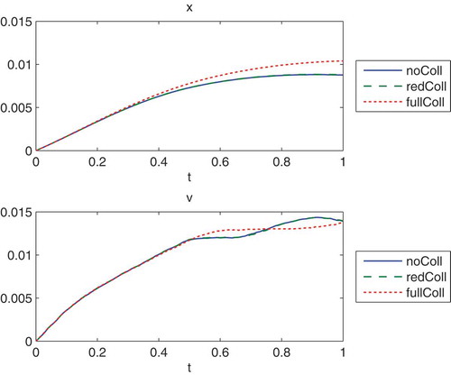
Figure 23. We present the field solutions of the space and velocity coordinates, given by $er{r}_{x,m,f}(t)=\left|{\mathbf{x}}_{ref,f}(t)-{\mathbf{x}}_{m,f}(t)\right|$ and $er{r}_{v,m,f}(t)=\left|{\mathbf{v}}_{ref,f}(t)-{\mathbf{v}}_{m,f}(t)\right|$ with $ref=reduced$ and $m=\left\{without,reduced,full\right\}$. In the figure, we compare the values of the particle $i=50$ with a fine computation of the full Coulomb collision model, also with particle $i=50$ and present the errors of the positions $x$ and velocities $v$.

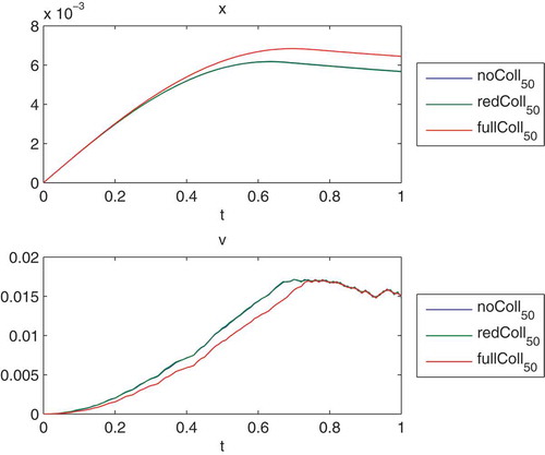
Remark 4.8 In the simulations, we see the benefit of the full model, which is stabler and allows shorter relaxation intervals. Overall, the benefit is also studied for long-time intervals and we see the flexibility of the modified model. We obtain a faster relaxation to the field-solutions of the space and velocity, see also [2]. Here the multiscale approach has the benefit of resolving in more detail the different collision functions.

5. Conclusion

We have presented a novel multiscale modelling method for plasma simulations based on the Fokker–Planck equation with Coulomb collision. The modelling allows separating the kinetic and the collision parts of the full model. Therefore, we model the multiscale problem in the transport part with multiple time scales and obtain a more accurate model. The model can be solved with correlated splitting schemes, namely, AB splitting and Hamiltonian splitting methods, so that the splitting of these physical processes is appropriate. We analysed the numerical schemes and discussed their symplecticity. Here, the Hamiltonian splitting conserves the symplecticity of the deterministic parts, whereas the AB splitting needs sufficiently small time steps and no blowing-up E-fields. While AB splitting schemes are natural to implement, we apply such a scheme to the full 6D model and simulate the transport problem in a common coordinate system (Cartesian system) and the collision problem in a local coordinate system (spherical system). Such a treatment allows applying fast solver methods, where we split it into a PIC method and an SDE method. In the numerical simulations we presented simplified 2D test problems and concluded that there was a benefit from combining the multiscale and splitting approaches. Such a flexibilization with the multiscale and splitting approaches allow to control the blow-up terms with a separate computation of the splitted equations with more adaptive time-steps. The adaptive control with finer time-steps and adequate time steps for each collision term allows to solve the problem with more accurate results. A full 6D test problem with ion–ion collisions of an Argon plasma has been studied. Here we obtain the benefit of an improved Coulomb collision model. The numerical studies were based on decomposing the collision function into different phases, so that in each collision phase an optimal collision function is computed. Further, we validated that the full collision model is possible and we can accelerate the computations. Such accelerations allow an implementation of such modified MPC algorithms to kinetic simulation packages in realistic problems of plasma processing, see [27,28] and [29]. In the future, we will focus on real-life applications with higher order splitting approaches to deal with larger time-steps, see [1].

Disclosure statement

No potential conflict of interest was reported by the author.

Appendix

The derivations of the models and splitting approaches are provided in the following appendix.

Appendix 1. The 2D model problem

We are motivated to study the multiscale model in a first, simpler, reduced transport–collision model, see [90].

For such a basic model equation, we reduce the phase-space to a two dimensional system with ($x,v$). The modelling equation is given in the following Fokker–Planck notation as

(121) $\frac{\mathrm{\partial }f}{\mathrm{\partial }t}+v\frac{\mathrm{\partial }f}{\mathrm{\partial }x}+E(x,ϵ)\frac{\mathrm{\partial }f}{\mathrm{\partial }v}=\frac{\mathrm{\partial }}{\mathrm{\partial }v}(-F_d(v)f+\frac{\mathrm{\partial }}{\mathrm{\partial }v}(D_v(v)f)),$(121)

where $f$ is the phase-space distribution function (density) of a charged plasma species. The particle is subjected to a multiscale E-field given by $E(x,ϵ)=ϵE_1(x)+E_{2}x$, where $ϵ\in [0,1]$, with $E_1(x)$ a non-linear function and $E_2$ the linear term, here in the two-dimensional equation it is a scalar. Further, $F_d$ is the convection function, also called the drag force, and $D_v$ is the diffusion function, see [2].

In the following, we introduce the standard 2D model problem, related to a one-scale solution to the zeroth order equation.

Appendix. 1.1. Standard 2D model problem

The simplified model can be studied in different ways:

• Splitting into a transport and collision part and solving the deterministic ODE with particle-in-cell (PIC) methods and the stochastic DE with an SDE solver.

• Applying the unsplit model and solving non-linear SDE equations.

Deterministic–stochastic splitting method for the 2D model

We can decouple such an FP equation into the PIC (particle in cell) part and the SDE (stochastic differential equation) part. For practical applications, this is necessary for higher dimensions and it is studied in [42] and [90].

For the 2D model we have the following parts:

• PIC part

(122) $\frac{dx}{dt}=v,$(122)

(123) $\frac{dv}{dt}=E(x,ϵ),$(123)

where $E(x,ϵ)=ϵ\frac{2}{x^2}-2x$ is the electric field and we assume a normalised parameter $\frac{q}{m}=1$, see [90].

• SDE part

(124) $dv=F_d(v)vdt+\sqrt{2D_v(v)}d{W}_v(t),$(124)

where $W_v$ is a Wiener process with $dW=\sqrt{dt}\xi$ and $\xi$ is a normally distributed random variable with $⟨\xi ⟩=0$, $⟨{\xi }^2⟩=1$, $F_d$ is the drag and $D_v$ is the diffusion coefficient, which are given in Equations (10)–(11).

Phase-space splitting (Hamiltonian splitting) method for the 2D model

We can decouple such equations into spatial and velocity equations. We split them into the following parts.

For the 2D model we have the following parts:

• Spatial part 1:

(125) $\frac{dx}{dt}=v,$(125)

where we apply a half time-step.

• Velocity part

(126) $dv=E(x,ϵ)dt+F_d(v)dt+\sqrt{2D_v(v)}d{W}_v(t),$(126)

where $E(x,ϵ)=ϵ\frac{2}{x^2}-2x$ is the electrical field and we use a normalizing parameter $\frac{q}{m}=1$. Further, $W_v$ is a Wiener process with $dW=\sqrt{dt}\xi$ and $\xi$ is a normally distributed random variable with $⟨\xi ⟩=0$, $⟨{\xi }^2⟩=1$. $F_d$ is the drag force coefficient and $D_v$ is the diffusion coefficient, which are given in Equations (10)–(11). We apply a full time-step for the equation and use the result of the spatial part 1 as the initial conditions.

• Spatial part 2:

(127) $\frac{dx}{dt}=v,$(127)

where we apply a half time-step and as initial conditions the results of the phase part and spatial part 1, see the Strang splitting or also the Hamiltonian splitting [24] and [22].

Non-splitting method for the 2D model

For such a reduction into a simpler 2D model, there is also the possibility of solving the two parts together, while there is no need to make a transformation between Cartesian and spherical coordinates. Further, such simplified models are faster to implement and it is not necessary to deal with large scale methods for each part (e.g. a fast independent PIC solver and a fast independent SDE solver).

We treat directly the multiscale non-linear SDE problem and apply an oscillatory and singular perturbed electric field $E(x,ϵ)$, see [42]:

(128) $\frac{dx}{dt}=v,$(128)

(129) $dv(t)=E(x,ϵ)dt+F_d(v)dt+\sqrt{2D_v(v)}dW,$(129)

where $W_v$ is a Wiener process with $dW=\sqrt{dt}\xi$ and $\xi$ is a normally distributed random variable with $⟨\xi ⟩=0$, $⟨{\xi }^2⟩=1$. $F_d$ is the drag force coefficient and $D_v$ is the diffusion coefficient, which are given in Equations (10)–(11).

Appendix 1.2. Multiscale 2D model problem

Here, we discuss the higher order expansion of the multiscale modelling problem.

We also study the multiscale modelling equations in two different ways:

• Splitting into a transport and collision part and solving with a deterministic ODE with particle-in-cell (PIC) methods and the stochastic DE with an SDE solver.

• Applying the unsplit model and solving a multiscale non-linear SDE equations.

Deterministic–Stochastic splitting method for the 2D model

We can decouple such an FP equation into the PIC (particle in cell) part and the SDE (stochastic differential equation) part. Such a practical application is necessary for higher dimensions and it is studied in [42] and [90].

For the 2D model we have the following parts:

• PIC part

(130) $\frac{d{x}_0(t)}{dt}=v_0,\frac{d{x}_1(t)}{dt}=v_1,$(130)

(131) $\frac{d{v}_0(t)}{dt}=E_2{x}_0(t),\frac{d{v}_1(t)}{dt}=E_1(x_0(t))+E_2{x}_1(t).$(131)

where $E(x,ϵ)=ϵ\frac{2}{x^2}-2x$ is the electrical field and we assume a normalizing parameter $\frac{q}{m}=1$, see [90].

• SDE part

(132) $d{v}_0=F_d(v_0(t))dt+\sqrt{2D(v_0(t))}d{W}_{v_0}(t),$(132)

(133) $d{v}_1=\frac{d{F}_d(v)}{dv}{|}_{v=v_0}{v}_{1}dt+\left({\left(2D(v)\right)}^{-1/2}\frac{dD(v)}{dv}\right){|}_{v=v_0}{v}_{1}d{W}_{v_0}(t),$(133)

where $W_v$ is a Wiener process with $dW=\sqrt{dt}\xi$ and $\xi$ is a normally distributed random variable with $⟨\xi ⟩=0$, $⟨{\xi }^2⟩=1$. Further, the drag force $F_d$ and the diffusion coefficient $D_v$ are given in Equations (10) and (11).

Phase-space splitting (Hamiltonian splitting) method for the 2D model

We can decouple such equations into spatial and velocity equations. We split them into the following parts.

For the 2D model we have the following parts:

• Spatial part 1:

(134) $\frac{d{x}_0(t)}{dt}=v_0,\frac{d{x}_1(t)}{dt}=v_1,$(134)

where we apply a half time-step.

• Velocity part

(135) $d{v}_0=E_2{x}_0(t)+F_d(v_0(t))dt+\sqrt{2D(v_0(t))}d{W}_{v_0}(t),$(135)

$d{v}_1=E_1(x_0(t))+E_2{x}_1(t)+\frac{d{F}_d(v)}{dv}{|}_{v=v_0}{v}_{1}dt+$

(136) $+\left(2{\left(D(v)\right)}^{-1/2}\frac{dD(v)}{dv}\right){|}_{v=v_0}{v}_{1}d{W}_{v_0}(t),$(136)

where $E(x,ϵ)=ϵ\frac{2}{x^2}-2x$ and we use a normalizing parameter $\frac{q}{m}=1$. Further, $W_v$ is a Wiener process with $dW=\sqrt{dt}\xi$ and $\xi$ is a normally distributed random variable with $⟨\xi ⟩=0$, $⟨{\xi }^2⟩=1$. Further, the drag force $F_d(v)$ and the diffusion coefficient $D_v$ are given in Equations (10)–(11). We apply a full time-step for the equation and use the result of the spatial part 1 as the initial conditions.

• Spatial part 2:

(137) $\frac{d{x}_0(t)}{dt}=v_0,\frac{d{x}_1(t)}{dt}=v_1,$(137)

where we apply a half time-step and as initial conditions the results of the phase part and spatial part 1, see the Strang splitting or also the Hamiltonian splitting [24] and [22].

Non-splitting method for the 2D model

For such a reduction into a simpler 2D model, there is also the possibility of solving the two parts together, while there is no need to do a transformation between Cartesian and spherical coordinates. Further, such simplified models are faster to implement and it is not necessary to deal with large scale methods for each part (e.g. a fast independent PIC solver and a fast independent SDE solver).

We treat directly the multiscale non-linear SDE problem and apply an oscillatory and singular perturbed electric field $E(x,ϵ)$, see [42]:

(138) $\frac{d{x}_0(t)}{dt}=v_0,\frac{d{x}_1(t)}{dt}=v_1,$(138)

(139) $d{v}_0=E_2{x}_0(t)+F_d(v_0(t))dt+\sqrt{2D(v_0(t))}d{W}_{v_0}(t),$(139)

$d{v}_1=E_1(x_0(t))+E_2{x}_1(t)+\frac{d{F}_d(v)}{dv}{|}_{v=v_0}{v}_{1}dt+$

(140) $+\left({\left(2D(v)\right)}^{-1/2}\frac{dD(v)}{dv}\right){|}_{v=v_0}{v}_{1}d{W}_{v_0}(t),$(140)

where $W_v$ is a Wiener process. Further, the drag force $F_d(v)v$ and the diffusion coefficient are given in Equations (10) and (11).

Appendix. 2 The non-splitting and splitting methods for the multiscale problems

In the following, we derive the underlying non-splitting and splitting methods for the multiscale problems.

The different schemes are given in the following.

Appendix 2.1. EM scheme

The application of the standard Euler–Maruyama scheme is given in Algorithm 8.

Algorithm 8 Euler{Maruyama scheme for solving the multiscale equations

• 1: Input: $x_{n,0},x_{n,1},v_{n,0},v_{n,1}{f}_{\alpha }(t^0)$ are the initial conditions. The time grid is given by $t^n$ with $n=0,\dots ,\tilde{N}$. $t^0$ is the initial time and $t^{\tilde{N}}=T$ the ending time.

• 2: for $n=0,\dots ,\tilde{N}-1$ do

• 3: EM scheme (non-splitting method)

(141) $x_{n+1,0}=x_{n,0}+v_{n,0}\mathrm{\Delta }t,$(141)

(142) $x_{n+1,1}=x_{n,1}+v_{n,1}\mathrm{\Delta }t,$(142)

(143) $v_{n+1,0}=v_{n,0}-2x_{n,0}\mathrm{\Delta }t+F_d(v_{n,0})\mathrm{\Delta }t+\sqrt{2D(v_{n,0})}\mathrm{\Delta }{W}_{v_0},$(143)

(144) $v_{n+1,1}=v_{n,1}-2x_{n,1}\mathrm{\Delta }t+\frac{2}{x_{n,0}^3}\mathrm{\Delta }t+\frac{d{F}_d(v)}{dv}{|}_{v=v_{n,0}}{v}_{n,1}\mathrm{\Delta }t+\left({\left(2D(v)\right)}^{-1/2}\frac{dD(v)}{dv}\right){|}_{v=v_{n,0}}{v}_{n,1}\mathrm{\Delta }{W}_{v_1}.$(144)

• 4: end for

• 5: The output is given by $x_{n+1,0},x_{n+1,1},v_{n+1,0},v_{n+1,1}$ for $n=1\dots ,\tilde{N}$.

Remark 6.1. For the EM scheme, which is an explicit time-discretization scheme, see [85], we have to restrict the time-steps:

(145) $\mathrm{\Delta }t\le min\left\{1,\sqrt{\frac{x_{n,0}^3{x}_{n,1}}{x_{n,0}^3{x}_{n,1}-1}},\frac{v_{n,0}}{\left|F_d(v_{n,0})\right|},\frac{1}{\left|\frac{d{F}_d(v)}{dv}{|}_{v=v_{n,0}}\right|}\right\},$(145)

where we assume $1.0\le x_{n,0}^3{x}_{n,1}$, $F_d(v_{n,0})\le 0$ and $\frac{d{F}_d(v)}{dv}{|}_{v=v_{n,0}}\le 0$ for all $n=0,\dots ,N$.

Appendix 2.2 Deterministic–stochastic splitting

• AB splitting

The application of the Deterministic–Stochastic AB splitting scheme is given in Algorithm 9.

Algorithm 9 AB splitting scheme

• 1: Input: $x_{n,0},x_{n,1},v_{n,0},v_{n,1}$ are the initial conditions. The time grid is given by $t^n$ with $n=0,\dots ,\tilde{N}$ with time-step $\mathrm{\Delta }t=t^{n+1}-t^n$. Further, we have intermediate time-steps for the stochastic scale with $\delta t=\frac{\mathrm{\Delta }t}{m}$. $t^0$ is the initial time and $t^{\tilde{N}}=T$ the ending time.

• 2: for $n=0,\dots ,\tilde{N}-1$ do

• 3: Step 1 (deterministic step, ODE)

(146) ${\tilde{x}}_{n+1,0}=x_{n,0}+v_{n,0}\mathrm{\Delta }t,$(146)

(147) ${\tilde{x}}_{n+1,1}=x_{n,1}+v_{n,1}\mathrm{\Delta }t,$(147)

(148) ${\tilde{v}}_{n+1,0}=v_{n,0}-2x_{n,0}\mathrm{\Delta }t,$(148)

(149) ${\tilde{v}}_{n+1,1}=v_{n,1}-2x_{n,1}\mathrm{\Delta }t+\frac{2}{x_{n,0}^3}\mathrm{\Delta }t,$(149)

• 4: Output: $x_{n+1,0},x_{n+1,1},v_{n+1,0},v_{n+1,1}.$

• 5: Input: $x_{n+1,0}={\tilde{x}}_{n+1,0},x_{n+1,1}={\tilde{x}}_{n+1,1},{\hat{v}}_{0,0}={\tilde{v}}_{n+1,0},{\hat{v}}_{0,1}={\tilde{v}}_{n+1,1}$ are the initial conditions.

• 6: for $p=0,\dots ,m-1$ do

• 7: Step 2 (stochastic step, SDE)

(150) ${\hat{v}}_{p+1,0}={\hat{v}}_{p,0}+F_d({\hat{v}}_{p,0})\delta t+\sqrt{2D({\hat{v}}_{p,0})}\delta W_{{\hat{v}}_0},$(150)

(151) ${\hat{v}}_{p+1,1}={\hat{v}}_{p,1}+\frac{d{F}_d(v)}{dv}{|}_{v={\hat{v}}_{p,0}}{\hat{v}}_{p,1}\delta t+\left({\left(2D(v)\right)}^{-1/2}\frac{dD(v)}{dv}\right){|}_{v={\hat{v}}_{p,0}}{\hat{v}}_{p,1}\delta W_{{\hat{v}}_1},$(151)

8: end for

The output is given by $v_{n+1,0}={\hat{v}}_{m,0},v_{n+1,1}={\hat{v}}_{m,1}$.

• 9: end for

• 10: The output is given by $x_{n+1,0},x_{n+1,1},v_{n+1,0},v_{n+1,1}$ for $n=1\dots ,\tilde{N}$.

Remark 6.2. For the deterministic–stochastic AB splitting scheme, which is a splitting approach, and separates the deterministic and stochastic operators, we have also in each part explicit time-discretization schemes, see [1,39,91] and [92].

We have to restrict the time-steps:

– Step 1 (A-part): Explicit Euler discretization:

(152) $\mathrm{\Delta }t\le min\left\{1,\sqrt{\frac{x_{n,0}^3{x}_{n,1}}{x_{n,0}^3{x}_{n,1}-1}}\right\},$(152)

where we assume $1.0\le x_{n,0}^3{x}_{n,1}$.

– Step 2 (B-part): Explicit Euler–Maruyama scheme (explicit time discretization):

(153) $\delta t\le min\left\{\frac{{\hat{v}}_{p,0}}{\left|F_d({\hat{v}}_{p,0})\right|},\frac{1}{\left|\frac{d{F}_d(v)}{dv}{|}_{v={\hat{v}}_{p,0}}\right|}\right\},$(153)

where we assume $F_d({\hat{v}}_{p,0})\le 0$ and $\frac{d{F}_d(v)}{dv}{|}_{v={\hat{v}}_{p,0}}\le 0$ and for all $p=0,\dots ,m-1$, see also [39].

Here, we have the benefit that the solver parts are separated, so that we can apply different time-steps for each part, see Figure 24

Figure 24. Different time-steps for the different A-B timescales in the AB splitting.

• ABA splitting scheme:

The application of the Deterministic–Stochastic ABA splitting scheme is given in Algorithm 10.

Algorithm 10 ABA splitting scheme

• 1: Input: $x_{n,0},x_{n,1},v_{n,0},v_{n,1}$ are the initial conditions. The time grid is given by $t^n$ with $n=0,\dots ,\tilde{N}$ with time-step $\mathrm{\Delta }t=t^{n+1}-t^n$. Further, we have intermediate time-steps for the stochastic scale with $\delta t=\frac{\mathrm{\Delta }t}{m}$. $t^0$ is the initial time and $t^{\tilde{N}}=T$ the ending time.

• 2: for $n=0,\dots ,\tilde{N}-1$ do

• 3: Step 1 (deterministic step, ODE)

(154) ${\tilde{x}}_{n+1,0}=x_{n,0}+v_{n,0}\mathrm{\Delta }t/2,$(154)

(155) ${\tilde{x}}_{n+1,1}=x_{n,1}+v_{n,1}\mathrm{\Delta }t/2,$(155)

(156) ${\tilde{v}}_{n+1,0}=v_{n,0}-2x_{n,0}\mathrm{\Delta }t/2,$(156)

(157) ${\tilde{v}}_{n+1,1}=v_{n,1}-2x_{n,1}\mathrm{\Delta }t/2+\frac{2}{x_{n,0}^3}\mathrm{\Delta }t/2,$(157)

• 4: Output: $x_{n+1,0},x_{n+1,1},v_{n+1,0},v_{n+1,1}$.

• 5: Input: $x_{n+1,0}={\tilde{x}}_{n+1,0},x_{n+1,1}={\tilde{x}}_{n+1,1},{\hat{v}}_{0,0}={\tilde{v}}_{n+1,0},{\hat{v}}_{0,1}={\tilde{v}}_{n+1,1}$ are the initial conditions.

• 6: for $p=0,\dots ,m-1$ do

• 7: Step 2 (stochastic step, SDE)

(158) ${\hat{v}}_{p+1,0}={\hat{v}}_{p,0}+F_d({\hat{v}}_{p,0})\delta t+\sqrt{2D({\hat{v}}_{p,0})}\delta W_{{\hat{v}}_0},$(158)

(159) ${\hat{v}}_{p+1,1}={\hat{v}}_{p,1}+\frac{d{F}_d(v)}{dv}{|}_{v={\hat{v}}_{p,0}}{\hat{v}}_{p,1}\delta t+\left({\left(2D(v)\right)}^{-1/2}\frac{dD(v)}{dv}\right){|}_{v={\hat{v}}_{p,0}}{\hat{v}}_{p,1}\delta W_{{\hat{v}}_1},$(159)

• 8: end for

• 9: The output is given by ${\hat{v}}_{m,0},{\hat{v}}_{m,1}$.

• 10: Input: ${\bar{x}}_{n+1,0}={\tilde{x}}_{n+1,0},{\bar{x}}_{n+1,1}={\tilde{x}}_{n+1,1},{\bar{v}}_{n+1,0}={\hat{v}}_{m,0},{\bar{v}}_{n+1,1}={\hat{v}}_{m,1}$ are the initial conditions.

• 11: Step 3 (deterministic step, ODE)

(160) $x_{n+1,0}={\bar{x}}_{n+1,0}+{\bar{v}}_{n+1,0}\mathrm{\Delta }t/2,$(160)

(161) $x_{n+1,1}={\bar{x}}_{n+1,1}+{\bar{v}}_{n+1,1}\mathrm{\Delta }t/2,$(161)

(162) $v_{n+1,0}={\bar{v}}_{n+1,0}-2{\bar{x}}_{n+1,0}\mathrm{\Delta }t/2,$(162)

(163) $v_{n+1,1}={\bar{v}}_{n+1,1}-2{\bar{x}}_{n+1,1}\mathrm{\Delta }t/2+\frac{2}{{\bar{x}}_{n+1,0}^3}\mathrm{\Delta }t/2.$(163)

• 12: end for

• 13: The output is given by $x_{n+1,0},x_{n+1,1},v_{n+1,0},v_{n+1,1}$ for $n=1\dots ,\tilde{N}$.

Remark 6.3. For the deterministic–stochastic ABA splitting scheme, which is a splitting approach, and separates the deterministic and stochastic operators, we have also in each part explicit time-discretization schemes, see [1,39,91] and [92].

We have to restrict the time-steps:

– Step 1 (A-part): Explicit Euler-discretization:

(164) $\mathrm{\Delta }t\le min\left\{1,\sqrt{\frac{x_{n,0}^3{x}_{n,1}}{x_{n,0}^3{x}_{n,1}-1}}\right\},$(164)

where we assume $1.0\le x_{n,0}^3{x}_{n,1}$.

– Step 2 (B-part): Explicit Euler–Maruyama scheme (explicit time discretization):

(165) $\delta t\le min\left\{\frac{{\hat{v}}_{p,0}}{\left|F_d({\hat{v}}_{p,0})\right|},\frac{1}{\left|\frac{d{F}_d(v)}{dv}{|}_{v={\hat{v}}_{p,0}}\right|}\right\},$(165)

where we assume $F_d({\hat{v}}_{p,0})\le 0$ and $\frac{d{F}_d(v)}{dv}{|}_{v={\hat{v}}_{p,0}}\le 0$ and for all $p=0,\dots ,m-1$, see also [39].

– Step 3 (A-part): Explicit Euler discretization:

(166) $\mathrm{\Delta }t\le min\left\{1,\sqrt{\frac{{\bar{x}}_{n,0}^3{\bar{x}}_{n,1}}{{\bar{x}}_{n,0}^3{\bar{x}}_{n,1}-1}}\right\},$(166)

where we assume $1.0\le {\bar{x}}_{n,0}^3{\bar{x}}_{n,1}$.

For the deterministic–stochastic AB and ABA splittings, we have the benefit of the flexibility of applying different time-steps in the A- or B-steps. Such a flexibility is important for fine resolutions and the short-time behaviour.

Appendix 2.3. Hamiltonian splitting

• AB Splitting

The application of the Hamiltonian AB splitting scheme, which is also known as the semi-implicit Euler method, see [15], uses Algorithm 11:

Algorithm 11 AB splitting scheme

• 1: Input: $x_{n,0},x_{n,1},v_{n,0},v_{n,1}$ are the initial conditions. The time grid is given by $t^n$ with $n=0,\dots ,\tilde{N}$ with time-step $\mathrm{\Delta }t=t^{n+1}-t^n$. Further, we have intermediate time-steps for the stochastic scale with $\delta t=\frac{\mathrm{\Delta }t}{m}$. $t^0$ is the initial time and $t^{\tilde{N}}=T$ the ending time.

• 2: for $n=0,\dots ,\tilde{N}-1$ do

• 3: Step 1 (symplectic step for $x$, ODE)

(167) ${\tilde{x}}_{n+1,0}=x_{n,0}+v_{n,0}\mathrm{\Delta }t,$(167)

(168) ${\tilde{x}}_{n+1,1}=x_{n,1}+v_{n,1}\mathrm{\Delta }t,$(168)

• 4: Step 2 (symplectic step for $v$, SDE)

(169) $v_{n+1,0}=v_{n,0}-2{\tilde{x}}_{n+1,0}\mathrm{\Delta }t+F_d(v_{n,0})\mathrm{\Delta }t+\sqrt{2D(v_{n,0})}\mathrm{\Delta }{W}_{v_0},$(169)

(170) $v_{n+1,1}=v_{n,1}-2{\tilde{x}}_{n+1,1}\mathrm{\Delta }t+\frac{2}{{\tilde{x}}_{n+1,0}^3}\mathrm{\Delta }t+\frac{d{F}_d(v)}{dv}{|}_{v=v_{n,0}}{v}_{n,1}\mathrm{\Delta }t+\left({\left(2D(v)\right)}^{-1/2}\frac{dD(v)}{dv}\right){|}_{v=v_{n,0}}{v}_{n,1}\mathrm{\Delta }{W}_{v_1},$(170)

• 5: end for

• 6: The output is given by $x_{n+1,0}={\tilde{x}}_{n+1,0},x_{n+1,1}={\tilde{x}}_{n+1,1},v_{n+1,0},v_{n+1,1}$ for $n=1\dots ,\tilde{N}$.

Remark 6.4. For the Hamiltonian AB splitting scheme, we also have explicit time-discretization schemes, see [15]. We have to restrict the time-steps as for the EM scheme, which is given in Equation (145), see [85] and [15].

• ABA Splitting ($x$-version)

The application of the Hamiltonian ABA splitting scheme ($x$-version), which is also known as the Störmer–Verlet method, see [15], uses the Algorithm 12:

Algorithm 12 ABA splitting scheme (x-version)

• 1: Input: $x_{n,0},x_{n,1},v_{n,0},v_{n,1}$ are the initial conditions. The time grid is given by $t^n$ with $n=0,\dots ,\tilde{N}$ with time-step $\mathrm{\Delta }t=t^{n+1}-t^n$. Further, we have intermediate time-steps for the stochastic scale with $\delta t=\frac{\mathrm{\Delta }t}{m}$. $t^0$ is the initial time and $t^{\tilde{N}}=T$ the ending time.

• 2: for $n=0,\dots ,\tilde{N}-1s$ do

• 3: Step 1 (symplectic step for $x$, ODE)

(171) ${\tilde{x}}_{n+1,0}=x_{n,0}+v_{n,0}\mathrm{\Delta }t/2,$(171)

(172) ${\tilde{x}}_{n+1,1}=x_{n,1}+v_{n,1}\mathrm{\Delta }t/2,$(172)

4: Step 2 (symplectic step for $v$, SDE)

(173) ${\hat{v}}_{n+1,0}=v_{n,0}-2{\tilde{x}}_{n+1,0}\mathrm{\Delta }t+F_d(v_{n,0})\mathrm{\Delta }t+\sqrt{2D(v_{n,0})}\mathrm{\Delta }{W}_{v_0},$(173)

(174) ${\hat{v}}_{n+1,1}=v_{n,1}-2{\tilde{x}}_{n+1,1}\mathrm{\Delta }t+\frac{2}{{\tilde{x}}_{n+1,0}^3}\mathrm{\Delta }t+\frac{d{F}_d(v)}{dv}{|}_{v=v_{n,0}}{v}_{n,1}\mathrm{\Delta }t+\left({\left(2D(v)\right)}^{-1/2}\frac{dD(v)}{dv}\right){|}_{v=v_{n,0}}{v}_{n,1}\mathrm{\Delta }{W}_{v_1},$(174)

5: Step 3 (symplectic step for $x$, ODE)

(175) $x_{n+1,0}={\tilde{x}}_{n+1,0}+{\hat{v}}_{n+1,0}\mathrm{\Delta }t/2,$(175)

(176) $x_{n+1,1}={\tilde{x}}_{n+1,1}+{\hat{v}}_{n+1,1}\mathrm{\Delta }t/2,$(176)

(177) $v_{n+1,1}={\hat{v}}_{n+1,1},$(177)

(178) $v_{n+1,1}={\hat{v}}_{n+1,1},$(178)

• 6: end for

• 7: The output is given by $x_{n+1,0},x_{n+1,1},v_{n+1,0},v_{n+1,1}$ for $n=1\dots ,\tilde{N}$.

• ABA Splitting ($v$-version)

The application of the Hamiltonian ABA splitting scheme ($x$-version), which is also known as Störmer–Verlet method, see [15], uses the Algorithm 13:

Algorithm 13 ABA splitting scheme (v-version)

• 1: Input: $x_{n,0},x_{n,1},v_{n,0},v_{n,1}$ are the initial conditions. The time grid is given by $t^n$ with $n=0,\dots ,\tilde{N}$ with time-step $\mathrm{\Delta }t=t^{n+1}-t^n$. Further, we have intermediate time-steps for the stochastic scale with $\delta t=\frac{\mathrm{\Delta }t}{m}$. is the initial time and $t^{\tilde{N}}=T$ the ending time.

• 2: for $n=0,\dots ,\tilde{N}-1$ do

• 3: Step 1 (symplectic step for $v$, SDE)

(179) ${\tilde{v}}_{n+1,0}=v_{n,0}-2x_{n,0}\mathrm{\Delta }t/2+F_d(v_{n,0})\mathrm{\Delta }t/2+\sqrt{2D(v_{n,0})}\mathrm{\Delta }{W}_{v_0}/\sqrt{2},$(179)

(180) ${\tilde{v}}_{n+1,1}=v_{n,1}-2x_{n,1}\mathrm{\Delta }t/2+\frac{2}{x_{n,0}^3}\mathrm{\Delta }t/2+\frac{d{F}_d(v)}{dv}{|}_{v=v_{n,0}}{v}_{n,1}\mathrm{\Delta }t/2+\left({\left(2D(v)\right)}^{-1/2}\frac{dD(v)}{dv}\right){|}_{v=v_{n,0}}{v}_{n,1}\mathrm{\Delta }{W}_{v_1}/\sqrt{2},$(180)

4: Step 2 (symplectic step for $x$, ODE)

(181) ${\hat{x}}_{n+1,0}=x_{n,0}+{\tilde{v}}_{n+1,0}\mathrm{\Delta }t,$(181)

(182) ${\hat{x}}_{n+1,1}=x_{n,1}+{\tilde{v}}_{n+1,1}\mathrm{\Delta }t,$(182)

5: Step 3 (symplectic step for $v$, SDE)

(183) $x_{n+1,0}={\hat{x}}_{n+1,0},$(183)

(184) $x_{n+1,1}={\hat{x}}_{n+1,1},$(184)

(185) $v_{n+1,0}={\tilde{v}}_{n+1,0}-2{\hat{x}}_{n+1,0}\mathrm{\Delta }t/2+F_d({\tilde{v}}_{n+1,0})({\tilde{v}}_{n+1,0})\mathrm{\Delta }t/2+\sqrt{2D({\tilde{v}}_{n+1,0})}\mathrm{\Delta }{W}_{{\tilde{v}}_0}/\sqrt{2},$(185)

(186) $v_{n+1,1}={\tilde{v}}_{n+1,1}-2{\hat{x}}_{n+1,1}\mathrm{\Delta }t/2+\frac{2}{{\hat{x}}_{n+1,0}^3}\mathrm{\Delta }t/2+\frac{d{F}_d(v)}{dv}{|}_{v={\tilde{v}}_{n+1,0}}{\tilde{v}}_{n+1,1}\mathrm{\Delta }t/2+\left({\left(2D(v)\right)}^{-1/2}\frac{dD(v)}{dv}\right){|}_{v={\tilde{v}}_{n+1,0}}{\tilde{v}}_{n+1,1}\mathrm{\Delta }{W}_{v_1}/\sqrt{2},$(186)

• 5: end for

• 6: The output is given by $x_{n+1,0},x_{n+1,1},v_{n+1,0},v_{n+1,1}$ for $n=1\dots ,\tilde{N}$.

Remark 6.5. For the Hamiltonian ABA splitting scheme, there are symplectic and explicit time-discretization schemes, see [15]. We also have to restrict the time-steps as for an EM scheme, which is given in Equation (145), see [85] and [15].

Based on the mixture of the deterministic and stochastic parts, it is not straightforward to use different time-steps for the A or B steps, while in the B steps, intermediate solutions are necessary. Therefore, we have to apply additional interpolation schemes to derive the intermediate solutions, for the ideas of such interpolation approaches, see [93].

Therefore the Hamiltonian splitting is used for large time intervals and we have the benefit of preserving the symplecticity, see [92].

Appendix 2.4. Improvements with the milstein scheme

An improvement can be attained using the Milstein scheme [26]. The next higher order correction with respect to an increase $\mathrm{\Delta }t/2$ to the Langevin equations for Coulomb collisions was derived.

We assume we are dealing with the 1D drag–diffusion equation, see also Equation (15) given by

(187) $dv(t)=a(v)dt+b(v)d{W}_v(t),$(187)

where $a$ is the drag coefficient, e.g. $a(v)=F_d(v)$ and $b$ is the diffusion coefficient, e.g. $b(v)=\sqrt{2D_v(v)}$. Then the Milstein scheme is applied to Equation (187) and given by

(188) $v^{n+1}=a(v^n)\mathrm{\Delta }t+b(v^n)\mathrm{\Delta }{W}_v+\frac{1}{2}b\frac{db}{dv}{|}_{v=v^n}(\mathrm{\Delta }{W}_v^2-\mathrm{\Delta }t),$(188)

where $v^n$ represents a velocity variable at time step $t^n$, and $\mathrm{\Delta }{W}_v$ is a Gaussian random variable with zero mean and variance $\mathrm{\Delta }t$. Further $\mathrm{\Delta }{W}^2$ is the square of $\mathrm{\Delta }W$. Here we obtain an order of $\mathcal{O}(\mathrm{\Delta }t)$ of the Milstein scheme, see [26].

In the next Example 6.1 we apply the additional Milstein term to our splitting approaches.

Example 6.1. We apply the additional term for the Milstein scheme in the Hamiltonian ABA splitting with Equation (185) and (186) and obtain

$v_{n+1,0}={\tilde{v}}_{n+1,0}-2{\hat{x}}_{n+1,0}\mathrm{\Delta }t/2$

$+F_d({\tilde{v}}_{n+1,0})({\tilde{v}}_{n+1,0})\mathrm{\Delta }t/2+\sqrt{2D({\tilde{v}}_{n+1,0})}\mathrm{\Delta }{W}_{v_0}/\sqrt{2},$

(189) $+\left(\frac{dD(v)}{dv}\right){|}_{v={\tilde{v}}_{n+1,0}}((\mathrm{\Delta }{W}_{v_0}/\sqrt{2}{)}^2-\mathrm{\Delta }t/2),$(189)

$v_{n+1,1}={\tilde{v}}_{n+1,1}-2{\hat{x}}_{n+1,1}\mathrm{\Delta }t/2+\frac{2}{{\hat{x}}_{n+1,0}^3}\mathrm{\Delta }t/2$

$+\frac{d{F}_d(v)}{dv}{|}_{v={\tilde{v}}_{n+1,0}}{\tilde{v}}_{n+1,1}\mathrm{\Delta }t/2+$

$+\left({\left(2D(v)\right)}^{-1/2}\frac{dD(v)}{dv}\right){|}_{v={\tilde{v}}_{n+1,0}}{\tilde{v}}_{n+1,1}\mathrm{\Delta }{W}_{v_1}/\sqrt{2},$

$+\left(-{\left(2D(v)\right)}^{-3/2}(\frac{dD(v)}{dv})2+2D(v)\frac{d^{2}D(v)}{d{v}^2}\right){|}_{v={\tilde{v}}_{n+1,0}}{\tilde{v}}_{n+1,1}\cdot$

(190) $\cdot ((\mathrm{\Delta }{W}_{v_0}/\sqrt{2}{)}^2-\mathrm{\Delta }t/2).$(190)

Remark 6.6. The multiscale solutions of the positions and velocities are reconstructed at the end of the algorithms, which are given by

(191) $x(t^{n+1},ϵ)=x_{n+1,0}+ϵx_{n+1,1},$(191)

(192) $v(t^{n+1},ϵ)=v_{n+1,0}+ϵv_{n+1,1}.$(192)

Such an additional behaviour allows computing separately the different multiscale parts and we can improve the solution with each additional multiscale term, see [1] and [13].

References

- J. Geiser, Modelling of Langevin equations by the method of multiple scales, IFAC-PapersOnLine 48 (1) (2015), pp. 341–345. doi:10.1016/j.ifacol.2015.05.001
- B.I. Cohen, A.M. Dimits, A. Friedman, and R.E. Caflisch, Time-step considerations in particle simulation algorithms for Coulomb collisions in plasmas, IEEE Trans. Plasma Sci. 38 (9) (2010), pp. 2394–2406. doi:10.1109/TPS.2010.2049589
- A.M. Dimits, B.I. Cohen, R.E. Caflisch, M.S. Rosin, and L. Ricketson, Higher-order time integration of Coulomb collisions in a plasma using Langevin equations, J. Comput. Phys. 242 (2013), pp. 561–580. doi:10.1016/j.jcp.2013.01.038
- K. Nanbu, Probability theory of electron–Molecule, ion–Molecule, molecule–Molecule, and Coulomb collisions for particle modeling of materials processing plasmas and cases, IEEE Trans. Plasma Sci. 28 (3) (2000), pp. 971–990. doi:10.1109/27.887765
- G. Gompper, T. Ihle, D.M. Kroll, and R.G. Winkler, Multi-Particle collision dynamics: A particle-based mesoscale simulation approach to the hydrodynamics of complex fluids, in Advanced Computer Simulation Approaches for Soft Matter Sciences III, C. Holm and K. Kremer, eds., Springer-Verlag, Berlin, 2009, pp. 1–87.
- R. Kapral, Multiparticle collision dynamics: Simulation of complex systems on mesoscales, in Stuart A. Rice, Advances in Chemical Physics, Wiley, 2008, pp. 89–146.
- M.A. Lieberman and A.J. Lichtenberg, Principles of Plasma Discharges and Materials Processing, Hoboken: Wiley, 2005.
- J.D. Lindl, P. Amendt, R.L. Berger, et al., The physics basis for ignition using indirect-drive targets on the national ignition facility, Phys. Plasmas 11 (2004), pp. 339–491. doi:10.1063/1.1578638
- D.C. Tidman and D.A. Montgomery, Plasma Kinetic Theory, McGraw-Hill, NY, 1964.
- L.D. Landau, The kinetic equation in the case of Coulomb interaction, Zh. Eksper. I Teoret. Fiz 7 (1937), pp. 203–209. (in German)
- H. Risken, The Fokker–Planck Equation: Methods of Solutions and Applications, Springer-Verlag, Berlin, 1996.
- K. Nanbu, Theory of cumulative small-angle collisions in plasmas, Phys. Rev. E, Stat. Phys. Plasmas Fluids Relat. Interdiscip. Top. 55 (4) (1997), pp. 4642–4652.
- J. Geiser, Multicomponent and Multiscale Systems—Theory, Methods, and Applications in Engineering, Springer-Verlag, Berlin, 2016.
- D.S. Lemons, D. Winske, W. Daughton, and B. Albright, Small-angle Coulomb collision model for particle-in-cell simulations, J. Comput. Phys. 228 (5) (2009), pp. 1391–1403. doi:10.1016/j.jcp.2008.10.025
- E. Hairer, C. Lubich, and G. Wanner, Geometric numerical integration illustrated by the StörmerVerlet method, Acta Numerica 12 (2003), pp. 399–450. doi:10.1017/S0962492902000144
- T. Shardlow, Splitting for dissipative particle dynamics, SIAM J. Sci. Comput. 24 (4) (2003), pp. 1267–1282. doi:10.1137/S1064827501392879
- M. Lisal, J.K. Brennan and J.Bonet Avalos. Dissipative particle dynamics at isothermal, isobaric, isoenergetic, and isoenthalpic conditions using Shardlow-like splitting algorithms, J. Chem. Phys. 135 (2011), pp. 204105. doi:10.1063/1.3660209
- G. Stoltz. Stable schemes for dissipative particle dynamics with conserved energy. Preprint, arXiv:1612.04154v2, 2017.
- E. Hairer and C. Lubich, Long-time energy conservation of numerical methods for oscillatory differential equations, SIAM J. Numer. Anal. 38 (2001), pp. 414–441. doi:10.1137/S0036142999353594
- E. Hairer, C. Lubich, and G. Wanner, Geometric Numerical Integration. Structure-Preserving Algorithms for Ordinary Differential Equations, Springer Series in Computational Mathematics, 2nd, Vol. 31, Springer, Berlin, Heidelberg, New-York, 2006
- J. Geiser, Decomposition Methods for Partial Differential Equations: Theory and Applications in Multiphysics Problems, CRC Press, Taylor & Francis, Boca Raton, London, New York, 2009.
- R.I. McLachlan and G.R.W. Quispel, Splitting methods, Acta Numerica 11 (2002), pp. 341–434.
- H.F. Trotter, On the product of semi-groups of operators, Proc. Am. Math. Soc. 10 (4) (1959), pp. 545–551. doi:10.1090/S0002-9939-1959-0108732-6
- G. Strang, On the construction and comparison of difference schemes, SIAM J. Numer. Anal. 5 (1968), pp. 506–517. doi:10.1137/0705041
- E. Hairer and G. Wanner, Solving Ordinary Differential Equations II, Springer-Verlag, Berlin, 1996.
- G.N. Milstein, Approximate integration of stochastic differential equations, Theory Probab. Appl. 19 (1974), pp. 552–562.
- J. Geiser and M. Arab, Porous media based modeling of PE-CVD apparatus: Electrical fields and deposition geometries, Spec. Top. Rev. Porous Media 1 (3) (2010), pp. 215–229. doi:10.1615/SpecialTopicsRevPorousMedia.v1.i3.30
- J. Geiser and M. Arab, Simulation of a chemical vapor deposition: Four phase model, Spec. Top. Rev. Porous Media 3 (1) (2012), pp. 55–68. doi:10.1615/SpecialTopicsRevPorousMedia.v3.i1.50
- V.I. Kobolov, FokkerPlanck modeling of electron kinetics in plasmas and semiconductors, Computational Mater. Sci. 28 (2003), pp. 302–320. doi:10.1016/S0927-0256(03)00115-0
- J. Geiser, Multiscale modeling of PE-CVD apparatus: Simulations and approximations, Polymers 5 (2013), pp. 142–160. doi:10.3390/polym5010142
- W.M. Manheimer, M. Lampe, and G. Joyce, newblock Langevin representation of Coulomb collisions in PIC simulations, J. Comput. Phys 138 (2) (1997), pp. 563–584. doi:10.1006/jcph.1997.5834
- T.K. Senega and R.P. Brinkmann, A multi-component transport model for non-equilibrium low-temperature low-pressure plasmas, J. Phys. D: Appl. Phys. 39 (2006), pp. 1606–1618. doi:10.1088/0022-3727/39/8/020
- K.-H. Spatschek, Theoretische Plasmaphysik, Teubner, Stuttgart, Germany, 1990.
- S. Chapman and T.G. Cowling, The Mathematical Theory of Non-Uniform Gases: An Account of the Kinetic Theory of Viscosity, Thermal Conduction, and Diffusion in Gases, Cambridge: Cambridge University Press, 1990.
- R.E. Robson, Introductory Transport Theory for Charged Particles in Gases, World Scientific, Singapore, 2006.
- M. Ohring, Materials Science of Thin Films, 2nd ed., Academic Press, San Diego, 2002.
- A.M. Dimits, B.I. Cohen, R.E. Caflisch, L. Ricketson, and M.S. Rosin. Higher-order and multi-level time integration of stochastic differential equations and application to Coulomb collisions. Lecture at Workshop III: Mathematical and Computer Science Approaches to High Energy Density Physics, May 7–11, 2012, IPAM, UCLA, USA, 2012.
- R. Hockney and J. Eastwood, Computer Simulation Using Particles, New York: CRC Press, 1985.
- P.E. Kloeden and E. Platen, The Numerical Solution of Stochastic Differential Equations, Springer-Verlag, Berlin, 1992.
- J. Geiser, Iterative Splitting Methods for Differential Equations, CRC Press, Taylor & Francis, Boca Raton, London, New York, 2011.
- G.A. Korn and T.M. Korn, Mathematical Handbook for Scientists and Engineers, McGraw-Hill, New York, 1961.
- N. Bou-Rabee and E. Vanden-Eijnden, A patch that imparts unconditional stability to explicit integrators for Langevin-like equations, J. Comput. Phys. 231 (2012), pp. 2565–2580. doi:10.1016/j.jcp.2011.12.007
- S. Chandrasekhar, Principle of Stellar Dynamics, Dover Publications, INC., Mineola, New York, 1960.
- L. Spitzer, Physics of Fully Ionized Gases, Wiley, NY, 1962.
- B. Oksendal, Stochastic Differential Equations: An Introduction with Applications, Springer-Verlag, Berlin, 2002.
- J. Cao, Statistical Mechanics, Spring (2012), Chapter 1, MIT OpenCourseWare, MIT, Cambridge http://ocw.mit.edu.
- M.P. Zorzano, H. Mais, and L. Vazquez, Numerical solution for Fokker–Planck equations in accelerators, Physica D 113 (2–4) (1998), pp. 379–381. doi:10.1016/S0167-2789(97)00292-3
- M.P. Zorzano, H. Mais, and L. Vazquez, Numerical solution of two dimensional Fokker–Planck equations, Appl Math Comput 98 (1999), pp. 109–117. doi:10.1016/S0096-3003(97)10161-8
- B. Leimkuhler and S. Reich, Simulating Hamiltonian Dynamics, Cambridge: Cambridge University Press, 2004.
- J. Kevorkian and J. Cole, Multiple Scale and Singular Perturbation Methods, Springer-Verlag, Berlin, 1996.
- J. Murdock, Perturbations: Theory and Methods, Hoboken: Wiley, 1991.
- M. Akimoto and A. Suzuki, Generalized entropies and the Langevin and Fokker-Planck equations, J. Korean Phys. Soc. 40 (6) (2002), pp. 974–978.
- B. Alexeev, Generalized Boltzmann Physical Kinetics, Elsevier, Amsterdam, 2004.
- R. Johnson, Singular Perturbation Theory, Springer-Verlag, Berlin, 2005.
- C. Kuehn, Multiple Time Scale Dynamics, Springer-Verlag, Berlin, 2015.
- B. Shivamoggi, Perturbation Methods for Differential Equations, Birkhäuser, Basel, 2003.
- G.A. Pavliotis and A.M. Stuart, Multiscale Methods: Averaging and Homogenization, Springer-Verlag, Berlin, 2008.
- T.D. Arber, R.G.L. Vann, and A. Critical, Comparison of Eulerian-Grid-based vlasov solvers, J. Comput. Phys. 180 (1) (2002), pp. 339–357. doi:10.1006/jcph.2002.7098
- F. Filbet and E. Sonnendrücker, Comparison of Eulerian Vlasov solvers, Comput. Phys. Commun. 150 (3) (2003), pp. 247–266. doi:10.1016/S0010-4655(02)00694-X
- B.I. Cohen, L. Divol, A.B. Langdon, and E.A. Williams, Effects of ion–Ion collisions and inhomogeneity in two-dimensional kinetic ion simulations of stimulated Brillouin backscattering, Phys. Plasmas 13 (2) (2006), pp. 022705. doi:10.1063/1.2168405
- M.S. Rosin, L.F. Ricketson, A.M. Dimits, R.E. Caflisch, and B.I. Cohen, Multilevel Monte Carlo simulation of Coulomb collisions, J. Comput. Phys. 274 (2014), pp. 140–157. doi:10.1016/j.jcp.2014.05.030
- N. Crouseilles, M. Mehrenberger, and E. Sonnendrücker, Conservative semi-Lagrangian schemes for the Vlasov equation, J. Comput. Phys. 229 (2010), pp. 1927–1953. doi:10.1016/j.jcp.2009.11.007
- V. Grandgirard, M. Brunetti, P. Bertrand, N. Besse, et al., A drift-kinetic semi-Lagrangian 4D code for ion turbulence simulation, J. Comput. Phys. 217 (2006), pp. 395–423. doi:10.1016/j.jcp.2006.01.023
- T. Takizuka and H. Abe, A binary collision model for plasma simulation with a particle code, J. Comput. Phys. 25 (3) (1977), pp. 205–219. doi:10.1016/0021-9991(77)90099-7
- M.E. Jones, D.S. Lemons, R.J. Mason, V.A. Thomas, and D. Winske, A grid-based Coulomb collision model for PIC codes, J. Comput. Phys. 123 (1) (1996), pp. 169–181. doi:10.1006/jcph.1996.0014
- M. Sherlock, A Monte-Carlo method for Coulomb collisions in hybrid plasma models, J. Comput. Phys. 227 (4) (2008), pp. 2286–2292. doi:10.1016/j.jcp.2007.11.037
- J. Geiser, Multiscale splitting for stochastic differential equations: Applications in particle collisions, J. Coupled Syst. Multiscale Dyn. 1 (2) (2013), pp. 241–250. doi:10.1166/jcsmd.2013.1017
- T. Ihle, E. Tüzel, and D.M. Kroll, Equilibrium calculation of transport coefficients for a fluid-particle model, Phys. Rev. E 72 (2005), pp. 046707. doi:10.1103/PhysRevE.72.046707
- E. Frenod, S.A. Hirstoaga, and E. Sonnendrücker, An exponential integrator for a highly oscillatory Vlasov equation, Discrete Continuous Dynamical Systems, Series S 8 (1) (2015), pp. 169–183. doi:10.3934/dcdss.2015.8.169
- N. Crouseilles, L. Einkemmer, and E. Faou, A Hamiltonian splitting for the Vlasov–Maxwell system, J. Comput. Phys. 283 (2015), pp. 224–240. doi:10.1016/j.jcp.2014.11.029
- E. Weinan, Principles of Multiscale Modelling, Cambrigde: Cambridge University Press, 2010.
- E. Weinan and B. Engquist, Multiscale modelling and computations, Notices of the AMS 50(9) (2003), pp. 1062–1070
- M. Griebel, S. Knapek, and G. Zumbusch. Numerical simulation in molecular dynamics: Numerics, algorithms, parallelization, applications. Texts in Computational Science and Engineering, Springer, Berlin, Heidelberg, New York, 2007.
- K.E. Gubbins and J.D. Moore, Molecular modeling of matter: Impact and prospects in engineering, Ind. Eng. Chem. Res. 49 (2010), pp. 3026–3046. doi:10.1021/ie901909c
- -A.-A. Homman, J.-B. Maillet, J. Roussel, and G. Stoltz, New parallelizable schemes for integrating the dissipative particle dynamics with energy conservation, J. Chem. Phys. 144 (2016), pp. 024112. doi:10.1063/1.4937797
- M.E. Innocenti, G. Lapenta, S. Markidis, A. Beck, and A. Vapirev, A multi level multi domain method for particle in cell plasma simulations, J. Comput. Phys. 238 (2013), pp. 115–140. doi:10.1016/j.jcp.2012.12.028
- J.P. Larentzos, J.K. Brennan, J.D. Moore, M. Lisal, and W.D. Mattson, Parallel implementation of isothermal and isoenergetic dissipative particle dynamics using Shardlow-like splitting algorithms, Comput. Phys. Commun. 185 (7) (2014), pp. 1987–1998. doi:10.1016/j.cpc.2014.03.029
- A.G.R. Thomas, M. Tzoufras, A.P.L. Robinson, R.J. Kingham, C.P. Ridgers, M. Sherlock, and A.R. Bell, A review of VlasovFokkerPlanck numerical modeling of inertial confinement fusion plasma, J. Comput. Phys 231 (3) (2012), pp. 1051–1079. doi:10.1016/j.jcp.2011.09.028
- L.J. Höök. Numerical solution of quasilinear kinetic diffusion equations in Toroidal plasmas. Doctoral Thesis, Trita-EE, KTH Royal Institute of Technology, 2013.
- K. Nanbu, T. Furubayashi, and H. Takekida, Coulomb collisions in materials processing plasmas, Thin Solid Films 506–507 (2006), pp. 720–723. doi:10.1016/j.tsf.2005.08.147
- J. Geiser and R. Röhle, Kinetic processes and phase-transition of CVD processes for Ti2SiC3, J. Convergence Inf. Technol. 5 (6) (2010), pp. 9–32. doi:10.4156/jcit
- J. Geiser, Multi-scale methods for transport problems: Theory and applications, in Computational Methods for Engineering Technology, Chapter 7, P. Ivanyi and B.H.V. Topping, eds., Saxe-Coburg Publications, Stirlingshire, Scotland, 2014, pp. 157–190.
- J. Geiser, V. Buck, and M. Arab, Model of PE-CVD apparatus: Verification and simulations, Math. Probl. Eng. 2010 (2010), pp. Article ID 407561. doi:10.1155/2010/407561
- V.S. Anishchenko, V. Astakhov, A. Neiman, T. Vadivasova, and L. Schimansky-Geier, Non-linear Dynamics of Chaotic and Stochastic Systems: Tutorial and Modern Developments, Springer-Verlag, Berlin, 2007.
- M. Liu, W. Cao, and Z. Fan, Convergence and stability of the semi-implicit Euler method for a linear stochastic differential delay equation, J. Comput. Appl. Math. 170 (2004), pp. 255–268. doi:10.1016/j.cam.2004.01.040
- J. Geiser, Iterative Splitting Methods for Coulomb Collisions in Plasma Simulations, Preprint, Cornell University Library, Ithaca, NY, arXiv:1706.06744, 2017
- J.A. Bittencourt, Fundamentals of Plasma Physics, 3rd ed., Springer-Verlag, Berlin, 2004.
- R. Fitzpatrick, Plasma Physics: An Introduction, CRC Press, Taylor & Francis, Boca Raton, FL, USA, 2015.
- J. Geiser and R. Röhle, Modeling and simulation for physical vapor deposition: Multiscale model, Int. J. Mathematical, Computational, Physical, Electrical Comput. Eng. 2 (11) (2008), pp. 816–824.
- J. Geiser, Model order reduction for numerical simulation of particle transport based on numerical integration approaches, Math. Comput. Model Dyn. Syst. 20 (4) (2014), pp. 317–344. doi:10.1080/13873954.2013.859159
- B. Leimkuhler and C. Matthews, Rational construction of stochastic numerical methods for molecular sampling, Appl. Math. Res. Express. 1 (2013), pp. 34–56.
- B. Leimkuhler and C. Matthews, The computation of averages from equilibrium and nonequilibrium Langevin molecular dynamics, IMA J. Numer. Anal. 36 (2016), pp. 13–79.
- J. Geiser, Iterative operator-splitting methods with higher order time-integration methods and applications for parabolic partial differential equations, J. Comput. Appl. Math. 217 (2008), pp. 227–242. doi:10.1016/j.cam.2007.06.028