On the modelling of heat exchangers and heat exchanger network dynamics using bond graphs

ABSTRACT

Heat exchanger networks are important systems in most thermal engineering systems and are found in applications ranging from power plants and the process industry to domestic heating. Achieving cost-effective design of heat exchanger networks relies heavily on mathematical modelling and simulation-based design. Today, stationary design calculations are carried out for all new designs, but for some special applications, the transient response of complete networks has been researched. However, simulating large heat exchanger networks poses challenges due to computational speed and stiff initial value problems when flow equations are cast in differential algebraic form. In this article, a systems approach to heat exchanger and heat exchanger network modelling is suggested. The modelling approach aims at reducing the cost of system model development by producing modular and interchangeable models. The approach also aims at improving the capability for large and complex network simulation by suggesting an explicit formulation of the network flow problem.

KEYWORDS:

• System simulation
• heat exchangers
• heat exchanger network
• bond graphs

1. Introduction

Heat exchanger networks (HENs) are essential components for thermal engineering systems such as power plants, most process systems, marine machinery systems and energy harvesting systems. When faced with the challenge of designing complex systems, a common approach is to use a simulation-based approach based on mathematical modelling of the total system and its components [1–3]. The heat exchanger is the main component of HENs, and the heat exchanger and system transient response is important with regard to both system optimisation and control. Papastratos et al. [4] investigated HEN dynamics as a part of a larger HEN design optimisation problem. The authors concluded that simulation of the heat exchanger dynamics is important when performing design optimisation to ensure that the system copes with dynamic operation conditions such as operation mode changes, startup and shutdown. Mathisen et al [5] investigated heat exchanger modelling with the goal of investigating HEN controllability. The authors argue that wall heat capacity may significantly affect dynamics, especially for gas phase heat exchange, and that pipe residence time is an important factor affecting the dynamics of HENs.

To achieve cost-effective system model development, a library of interchangeable, reusable component models of appropriate fidelity needs to be available. According to the evaluation of different modelling approaches by Vangheluwe [6], this is best achieved by using bond graphs. Bond graph modelling is a unifying approach suitable for multi-domain modelling and model interchangeability. In addition, component connectivity and causality are visualised.

Several suggestions for thermofluid bond graph modelling have been put forward. Thoma [7,8] introduced a true bond graph using temperature as the effort variable and entropy flow as the flow variable for representing energy flow. Brown [9] introduced a bond graph with two effort variables and one flow variable. Stagnation enthalpy and pressure were chosen as effort variables and mass flow as the flow variable to represent the flow of energy and mass. Karnopp [10] introduced thermofluid pseudo bonds for modelling thermofluid systems. Here, the energy flow is represented by two bonds, one hydraulic and one pseudo thermal bond. The pseudo thermal bond has thermal energy flow as the flow variable and temperature as the effort variable. Several heat exchanger models using the approach of Thoma have been presented [11–13]. However, due to the unconventional nature of entropy flow calculation, the authors chose to use the pseudo bond graph thermofluid approach of Karnopp.

The use of pseudo thermofluid bonds to model heat exchangers is presented in several publications. Bentaleb et al. [14] presented a lumped bond graph model for a plate heat exchanger (PHE) using thermofluid pseudo bonds. The heat exchanger consists of a multiport Cfields with R-fields connecting upstream and downstream fluid lumps. The Cfields calculate pressure and temperature based on the accumulated mass and energy. Hot and cold sides are connected through an R-element determining the heat flow. A heat exchanger model is configured by connecting several heat exchanger elements in series. The challenge with this approach, when using liquids as the working medium, is that the system becomes very stiff due to the incompressible nature of liquids. This approach is therefore not well suited for system simulations in which simulation times of minutes to hours are of interest.

Borutzky [15] presented a lumped pseudo bond graph of a simple counter flow heat exchanger. His model consists of one thermal lump for the hot side and one for the cold side. The hydraulic flow and thermal flow are partly split. Hydraulic flow and thermal flow are connected with a flow signal from the hydraulic side, which is used to calculate the heat transfer due to advection. Heat transfer between the hot and cold side is determined based on the logarithmic mean temperature. In addition, a valve is used to control one of the hydraulic flows. Representing hot and cold side by single lumps and using the logarithmic mean temperature difference lacks the capability of capturing the effect of internal flow patterns on the heat exchanger transient response. Real heat exchangers normally have complex flow patterns that require additional lumps to capture a more detailed thermal transient response. In addition, using the logarithmic mean temperature difference requires additional logic for simulation of startup and shutdown or other scenarios where the hot and cold side temperatures are equal. A single control valve in the flow to a heat exchanger is not a common way of controlling the outlet temperature. Using a heat exchanger bypass and a three way valve is the standard approach, which will be shown to present challenges when formulating the hydraulic flow problem.

Engja [16] presented a shell and tube heat exchanger (STHE) model with the goal of capturing the flow patterns of more complex heat exchanger designs. This is achieved by dividing each thermal flow into several thermal lumps, with divisions between sections with counter, parallel or cross flow. Previous time step temperatures were used without compromising accuracy for the calculation of heat transfer rates, removing the need for thermal lumps representing the heat exchanger wall. The need for a wall temperature model is due to heat transfer coefficients being dependent on the wall temperature, and the wall temperature depends on the heat transfer rate, resulting in an algebraic loop.

Several computational challenges arise when connecting models of components, such as heat exchangers and valves, to form a heat exchanger network model. With the assumption that pressure drop is included in the hydraulic part of the heat exchanger and valve models, component-to-component connection leads to a hydraulic network flow problem. Steady state flow calculations in hydraulic networks are solved by iterative methods [17], where stiff initial value problems make guessing initial values challenging. Using this formulation of hydraulic flow in simulations leads to differential algebraic equations (DAE). Such equations may be computationally costly to solve, especially for large complex systems. In addition, computational problems may occur for situations in which a valve closes, resulting in infinite flow losses. This article will present an approach in which simple model modifications based on introducing fluid compliance between components will result in explicit formulations of the flow equations and, as such, support a modular component-based modelling approach.

The novelty of the method proposed is the ability to model HENs in a consistent manner based on library components, where the final hydraulic flow formulation is cast in an explicit form. The approach is suitable for simulation-based design of complex systems.

In Section 2, examples of typical heat exchanger models are presented. Additional challenges related to modelling HENs are discussed, and the approach for explicit formulation is presented. Section 3 presents examples of the modelling approach, while discussions and the conclusion are found in Section 4.

2. Model development

2.1. Heat exchanger modelling

To achieve the goal of efficient and consistent model development, heat exchanger modelling is based on the bond graph formalism and a control volume representation of the heat exchanger. The mathematical description of the physical processes is based on 1D mass and heat transfer modelling. This leads to a lumped model formulation in which bond graph elements representing physical processes, such as heat transfer and lumped fluid flows, are the basic building blocks for modelling different types of heat exchangers. Hydraulic flow is assumed to be incompressible with a constant flow rate throughout the heat exchanger. In addition, a physical modelling approach to mathematical formulation is used to ensure simulation capability of startup, shutdown, reverse flow, control systems and changes in flow topology due to changes in valve positions. The thermal transient response of different types of heat exchangers is captured by how the bond graph elements are combined to represent a heat exchanger heat and mass transfer flow pattern.

Four bond graph elements are used to capture the mass and heat transfer process: thermal lumps C, heat transfer $R_C$ elements for convection and conduction, thermal flux $R_{\dot{V}}$ elements for heat transfer between thermal lumps by advection, and a hydraulic pressure drop element R. Figure 1 shows a generic connection of three thermal lumps representing flow one, the material in the separating wall and flow two. The dashed bonds represent the heat transfer. Solid bonds represent the hydraulic flow.

Figure 1. Generic bond graph model for heat transfer through a material separating hot and cold flows. Solid bonds represent hydraulic flow, while dashed bonds represent the flow of thermal energy. Flows are assumed to be incompressible.

With the resulting causalities mass flow is given by the pressure drop

(1) $\dot{m}=f(\mathrm{\Delta }P)$(1)

while heat transfer by advection or convection is a function of the temperature difference and mass flow

(2) $\dot{Q}=f(\mathrm{\Delta }T,\dot{m})$(2)

As hydraulic flow is not connected to the thermal energy flow, $\dot{m}$ is distributed as a signal to all elements requiring the mass flow as input. Energy accumulated in the thermal lumps is given by the integral net energy flow in and out of the control volume.

(3) $\frac{dQ}{dt}=\int \sum _{i=1}^n{\dot{Q}}_i$(3)

Heat transfer by advection in $R_{\dot{V}}$ elements between adjacent thermal lumps is determined by the mass flow rate and the temperature of the upstream thermal lump.

(4) ${\dot{Q}}_{\dot{V}i}=\frac{\dot{m}}{2}cp\left(T_{\left(i+1\right)}-T_i\right)+\frac{\left|\dot{m}\right|}{2}cp\left(T_{\left(i+1\right)}+T_i\right)$(4)

Heat transfer due to convection and conduction between a thermal lump and a wall lump is determined by the temperature difference, the convection heat transfer coefficient $h$, the area of heat transfer $A$, half the wall lump thickness $d_w$ and the thermal conductivity of the wall material $k_w$,

(5) ${\dot{Q}}_{Ci}=\frac{T_i-T_{wi}}{1/hA+d_w/k_{w}A}$(5)

For Biot numbers below 0.1 the error of using a single wall lump is small [18]. However, additional lumps or other models such as finite difference may be used for cases where Biot number is above 0.1 and transient wall heat transfer have a significant effect on the transient response of the heat exchanger performance. Time dependent heat transfer through the wall is captured by the change in wall lump temperature when wall boundary temperatures change. Temperature profiles through the wall for one and three wall lumps are given in Figure 2 where $T_w$ is the temperature calculated in the wall lumps.

Figure 2. Temperature profiles between hot and cold liquid through the wall with two liquid control volumes for a single wall control volume and for three wall control volumes.

Empirical correlations for the heat transfer and the pressure drop for different types of heat exchangers are available in the literature, e.g. [19]. Using appropriate correlations is a modelling decision where limitations on flow regimes, temperature differences and geometry should be considered. Guidance to selection of appropriate correlations would be beneficial if implemented in a modelling tool, however such a feature is not considered in this study. The modelling structure suggested does not lock the modeller into specific empirical relationships or specific modelling assumptions. Limitations that are imposed are those that arise from using a lumped modelling approach.

The presented basic bond graph element building blocks can be combined to represent the various flow patterns found in different types of heat exchangers. Identifying appropriate control volumes is an important task when modelling heat exchangers and requires some experience. Selecting control volumes for which there are relatively small variations in temperature and flow velocity within the control volume allows for calculation of heat transfer coefficients with small errors for the control volume. This is achieved by selecting control volumes with either parallel, counter or cross flow. For large sections of parallel, counter or cross flow, several control volumes may be required to capture the transient response.

Models for a typical STHE and a PHE are presented as examples. Schematic diagrams for the example heat exchangers are given in Figure 3.

Figure 3. Heat exchanger schematics for (a) a shell and tube heat exchanger with baffles, (b) an U-arranged plate heat exchanger.

2.1.1. Shell and tube heat exchanger

A typical STHE consists of an outer shell with internal baffles directing fluid flowing in the shell across and partially along a bank of tubes. Different standard designs are designated according to the Tubular Exchanger Manufacturers Association (TEMA) classification. The STHE considered here is a two pass tube, baffled single pass shell heat exchanger. Due to the baffles and the two pass tube flow arrangement, the flow in the shell alternates between flowing through the turn and return tube banks. A reasonable approach is to divide the shell side into control volumes between two baffles and to apply a division in the longitudinal direction between the turn and return banks of the tubes. The same division is also done for the tube side with the addition of a control volume at the rear end.

A bond graph example of a heat exchanger with two baffles is given in Figure 4. Only the thermal bonds are included to increase readability. As the bond graph is somewhat complicated, all shell thermal lumps have been designated $C_s$, all pipe thermal lumps $C_p$ and all wall lumps $C_w$.

Figure 4. Thermal bonds for a shell and tube heat exchanger with two pass tube flow, single pass shell flow and two baffles.

2.1.2. Plate heat exchanger

PHEs consist of four ports representing inlets and outlets for hot and cold liquid streams. The ports distribute and collect the streams to and from small channels between the plates, with hot and cold streams flowing in alternate channels. The PHE may be divided into $n\times m$ sections, where each section contains three thermal lumps, hot and cold streams and the heat exchanger wall. $n$ is the number of horizontal divisions, and $m$ is the number of vertical divisions. The number of horizontal and vertical divisions needed depends on the accuracy requirements for transient prediction. Depending on the selected number of divisions, several plates and channels are combined together in a single lump. In addition, thermal lumps for the ports have to be included.

A PHE model with $2\times 2$ sections is presented in Figure 5. Only the thermal bonds are included to increase readability.

Figure 5. Bond graph representation of a U-arranged plate heat exchanger.

2.2. Heat exchanger network modelling

With the suggested modelling approach, the thermal transient response within a heat exchanger is captured by spacial discretization of the heat exchanger with thermal lumps. The transient response due to changes in the HEN flow and flow distribution is, however, determined by the network of connected hydraulic R-elements. Each R-element represents a component with a pressure drop such as a heat exchanger or a flow passage. This direct component-to-component connection with only R-elements leads to DAEs. This problem resembles the flow calculation problem known from the calculations of hydraulic networks. In hydraulic network flow problems, mass conservation in junctions is established based on a law equivalent to Kirchhoff’s current law, while mass or volume flows are calculated between junctions based on non-linear pressure drop equations. This system of non-linear equations has to be solved using an iterative method [20]. The convergence rate depends on the system topology, iteration method and selection of initial values [21,22]. The initial values are often required to be very close to the solution for the iteration method to guarantee the correct solution. Simulation of large systems of DAEs often results in a slow computational speed due to the large system of algebraic equations that needs to be solved iteratively at each time step.

This study proposes the introduction of bulk modulus compliance C-elements at 0-junctions and between series-connected hydraulic pressure drop R-elements. The bulk modulus C-element has accumulated mass as the state and calculates the pressure based on the bulk modulus of the liquid.

(6) $C=\frac{V}{\beta }$(6)

where V is the volume and $\beta$ is the bulk modulus. With this approach, pressure is calculated at every node and between series-connected R-elements, resulting in flow out causality for all R-elements and explicit formulation of the hydraulic flow problem. The goal of the proposed approach is to increase the simulation speed and allow for flexible system model assembly and increased flexibility in selecting the initial values. It should be noted that the R-element flow out causality will require an iterative solution of the pressure drop equation.

This approach resembles the approach of [23], in which the authors suggested using simulation instead of iteration to solve stationary hydraulic network flow problems. Their approach was to include the bulk modulus of the pipes to determine the pressure at nodes, combined with a relation giving the flow rate as a function of the pressure drop in pipes. Simulations were run until a steady state was achieved. A key difference between the use of the bulk modulus to calculate the pressure at nodes for heat exchanger networks and the typical applications of hydraulic network flow is the size and length of pipes. Typical applications of hydraulic network flow involve city water distribution systems with large pipe diameters and long pipe lengths. HENs typically have much shorter pipes and smaller diameters, which have a significant effect on the time constants $\tau$ in the system. The time constant is determined by the bulk modulus, pressure drop and volume.

(7) $\tau =\frac{\beta }{RV}$(7)

where $R$ is the pressure drop as a function of flow rate $[\frac{\mathrm{k}\mathrm{P}\mathrm{a}}{{\mathrm{m}}^3/\mathrm{s}}]$ and $V$ is the geometric volume. The time constant of the bulk modulus of liquids is generally very small, which poses a computation speed challenge. One method to reduce the system stiffness is to reduce the bulk modulus value to levels that give both a high simulation speed and negligible errors in the simulation results. However, care must be taken, and the simulation result validity must be checked. The effect of changing the value of the bulk modulus on the simulation results and the simulation speed will be explored in the next section.

The introduction of bulk modulus C-elements also solves a potential mathematical problem when using three way valves in hydraulic network flow problems. A typical valve pressure drop equation is a function of the valve area $A$, mass flow rate $\dot{m}$ and discharge coefficient $C_d$.

(8) $\mathrm{\Delta }P=\frac{{\dot{m}}^2}{2C_d^2{A}^2}$(8)

Flow area $A$ and $C_d$ are functions of the three way valve rotor position. In this form, the equation has effort out causality. For cases where flow out causality is required, the inverse flow out relationship is used.

(9) $\dot{m}=\sqrt{2\mathrm{\Delta }P{C}_d^2{A}^2}$(9)

However, division by zero will occur if the valve closes completely ($A=0$) for effort out causality. When using bulk modulus C-elements, the effort out causality is avoided, allowing the valve to close completely for both bypasses and heat exchanger loops.

In addition, the bulk modulus C-element can be expanded to a pipe model capturing temperature transport delay by using additional thermal lumps. Transport behaviour is dependent on the number of thermal lumps. Figure 6 presents a pipe model with a C-element for the bulk modulus and three thermal lumps for thermal energy transport. As the amount of liquid in the pipe is determined by the geometric volume of the pipe and the bulk modulus calculation, the second thermal control volume is used to correct for the change in fluid mass in the pipe caused by the change in pressure. The masses of thermal control volumes one and three are constant. The pipe model may easily be expanded to include the heat capacity of the pipe walls and the thermal energy exchange with the surroundings.

Figure 6. Bond graph representation of a pipe.

An example of the use of the bulk modulus C-element is presented for a heat exchanger bypass used for temperature control. The temperature is controlled by a three way valve controlling the flow through two heat exchangers in parallel. Possible causality assignment is presented in Figure 7, where elements $M{R}_1$ and $M{R}_2$ represent the three way valve and $R_1$ and $R_2$ represent the heat exchangers.

Figure 7. Heat exchanger bypass flow arrangement with parallel heat exchangers being controlled. Some examples of causality assignments are given in the subfigures, where all assignments results in algebraic loops.

When adding bulk modulus C-elements, as shown in Figure 8, all pressure drop R-elements have flow out causality, resolving the algebraic loop.

Figure 8. Heat exchanger bypass with bulk modulus C-elements and parallel heat exchangers.

3. Simulation and results

In this section two modelling and simulation cases and a comparison with steady state measurement data are presented. The first case compares two STHE with different layouts evaluating the effect on transient response. The second case looks at HEN modelling and simulation where the use of bulk modulus compliance C-elements is investigated and evaluated.

Some common assumptions are made for the models developed in this section. Based on the use of incompressible fluid and a limited temperature range thermal conductivity and diffusivity, specific heat capacity and fluid density are assumed constant and independent of fluid temperature. Viscosity is temperature dependent and is calculated based on exponential curve fitting. Heat transfer correlations are only included for turbulent flow and does not take into account developing flow. If the effect of developing flow is to be considered, this have to be implemented as corrections to the heat transfer coefficients in the affected thermal lump. It is also assumed that heat transfer is dominated by the convection at the wall surfaces and that the temperature difference over the wall is small, resulting in a negligible error from using a single wall thermal lump.

For STHE models used in this section, the authors have chosen to use Gnielinski’s correlation [24] for tube side Nusselt number and the correlation suggested by McAdams for shell side heat transfer coefficient [25]. Laminar flow is not considered. For the shell side pressure drop the Kern method [26] is used while the Blasius equation is used for the tube side. For PHEs Wang and Sunden Nusselts number correlations and Fanning friction factor have been implemented [27].

Although no thorough model verification process has been undertaken at this time, a comparison with an available data set has been carried out. The data set is for an STHE lubrication oil cooler at a single steady state operation point. Heat exchanger data is available in Table 1 Results from simulation with the suggested modelling approach are found in Table 2. The comparison is found to show small differences between the measurement and simulation data.

Table 1. Data set for measured STHE used for comparison of steady state model prediction.

Parameter	Value
Shell diameter	382[mm]
Tube outer diameter	12.7 [mm]
Tube inner diameter	10.7 [mm]
Centre tube to tube distance	16.5 [mm]
Pitch	Rectangular
Tube length	1500 [mm]
Number of baffles	7
Number of tube passes	2
Tubes per pass	206
Tube liquid	Sea water
Shell liquid	Lubrication oil
Lubrication oil inlet temperature	60.2 [C${ }^{\circ }$]
Sea water inlet temperature	6.2 [C${ }^{\circ }$]
Lubrication oil outlet temperature	47.5 [C${ }^{\circ }$]
Sea water outlet temperature	11.0 [C${ }^{\circ }$]
Lubrication oil flow rate	12.2 [kg/s]
Sea water flow rate	14.8 [kg/s]

Table 2. Comparison between simulation and measured data.

	Lubrication oil outlet	Sea water outlet
Measured values	11.0 [C${ }^{\circ }$]	47.5 [C${ }^{\circ }$]
Simulation results	11.4 [C${ }^{\circ }$]	47.5 [C${ }^{\circ }$]

3.1. Shell and tube heat exchanger layout comparison

A case where two STHE with different flow arrangements is compared has been selected with the aim of demonstrating the ability of the modelling approach to capture effect of design geometry on transient response. The first design is a four pass, three baffle heat exchanger, while the second design is a two pass, six baffle heat exchanger. The two designs have approximately equal total heat transfer with equal flow rates. Features that are different for the two designs are given in Table 3. Other design features are not changed.

Table 3. Design features difference between the four pass three baffle and two pass six baffle STHE design.

Design feature	2 pass 6 baffles	4 pass 3 baffles
Number of tubes	313	626
Shell diameter	0.353 [m]	0.50 [m]
Tube length	1.2 [m]	0.6 [m]

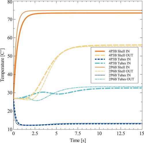
The simulation case selected is heat exchanger startup where all temperatures are equal throughout the heat exchanger at the initial time. At time 0 flow and temperature stepped to operation conditions. Figure 9 shows the transient response for the first and last thermal lumps of shell and tube flow for the two designs. The model predicts different transient response for the two designs before reaching approximately the same steady state temperature, however at different times.

Figure 9. Comparison of two STHE layouts, 4 pass 3 baffles (4P3B) and 2 pass 6 baffles (2P6B), during start up.

3.2. Heat exchanger network modelling

An example of the suggested HEN system modelling approach has been implemented and simulated. The goal of the simulation example is to compare the effect of different values of the bulk modulus on temperature and mass flow results and the simulation speed. The example is based on the bypass arrangement in Figure 8 with two parallel PHEs.

The bypass valve is controlled by a PI controller with a set point of 309 K. Both the cold and warm side inlet temperatures vary harmonically with different frequencies to ensure that the bypass valve closes both the bypass loop and the heat exchanger loop. The simulation scenario starts at 0 s and ends at 60 s. Temperature and mass flow results are plotted in Figure 10. The differences between using a bulk modulus of 2.2e9 and the modified bulk modulus values are plotted in Figure 11, while the simulation speed results are given in Table 4.

Table 4. Comparison of simulation speeds for a 60 s scenario with different values of the bulk modulus. Simulation time in seconds on a standard laptop computer.

Bulk modulus [Pa]	Simulation speed (times faster)	Simulation time [s]
2.2e9	1	108.1
2.2e8	20	5.5
2.2e7	35	3.1
2.2e6	120	0.9
2.2e5	272	0.4

Figure 10. Simulation results for mass flow in hot flow heat exchanger one, the bypass temperature out and the cold flow temperature out. Comparison of the effect of different values of the bulk modulus on the simulation results. Flow 1 is the flow controlled by the bypass valve (hot), while Flow 2 is the uncontrolled flow in the heat exchangers (cold).

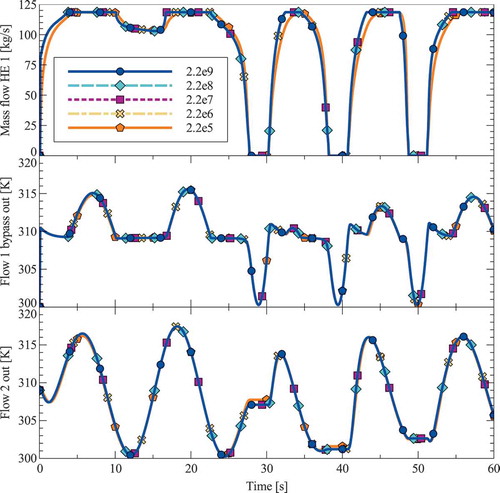
Figure 11. Simulation results for mass flow in hot flow heat exchanger one, the bypass temperature out and the cold flow temperature out. Difference between results when using a bulk modulus of 2.2e9 and modified bulk modulus values.

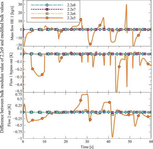
Relatively no effect on mass flow and temperature is found before a bulk modulus of 2.2e5 is simulated. However, significant simulation time gains are achieved with every reduction of the bulk modulus. Robust results and significantly increased simulation speeds are found for bulk modulus values in the range of $1\cdot {10}^6-1\cdot {10}^7$, which are recommended as a best practice.

4. Discussion and conclusion

The modelling approach suggested allows for easy assembly of complex HEN models for which all required sub-model modules are available in a common modelling framework. Different types of heat exchangers have been developed. The modelling framework fits the requirement for interchangeable and reusable models of appropriate fidelity for system simulation by ensuring compatible interfaces. The use of bond graphs allows for connection to additional models of components common to thermal power systems. This allows for the investigation of coupled effects in complex engineering systems. The use of bond graphs also highlights numerical issues with model assembly such as algebraic loops and requirements for internal iterations. The use of bulk modulus control volumes to resolve these algebraic loops is put forward as a method to resolve these algebraic loops. However, introducing bulk modulus control volumes is not without challenges, as they may introduce very small time constants. To mitigate this problem, the time constants have to be modified by reducing the value of the bulk modulus. The use of bulk modulus values in the range of $1\cdot {10}^6-1\cdot {10}^7$ was found to produce significant improvement of the simulation speed without any significant negative effect on the heat exchanger performance predictions. This again allows for assembly of larger more complex networks without exponential growth in computational power requirements.

Acknowledgments

This work was carried out at SFI Smart Maritime, which is mainly supported by the Research Council of Norway through the Centres for Research-based Innovation (SFI) funding scheme, project number 237917.

Disclosure statement

No potential conflict of interest was reported by the authors.

Additional information

Funding

This work was supported by the Norges Forskningsråd [237917]

References

- C. Paredis, A. DiazCalderon, R. Sinha, and P. Khosla, Composable models for simulationbased design, Eng. Comput. 17 (2001), pp. 112–128. Available at http://link.springer.com/10.1007/PL00007197.
- P.T. Hewlett and T.M. Kiehne, Dynamic simulation of shipsystem thermal load management, in 6th annual IEEE Conference on Automation Science and Engineering, Toronto, Canada, 2010, pp. 734–741.
- S. Yang, J. Ordonez, J. Vargas, J. Chalfant, and C. Chryssostomidis, Systemlevel ship thermal management tool for dynamic thermal and piping network analyses in earlydesign stages, in IEEE Electric Ship Technology Symposium, Vol. 2956, Arlington, VA, 2017, pp. 501–507.
- S. Papastratos, A. Isambert, and D. Depeyre, Computerized optimum design and dynamic simulation of heat, Computers Chem. Eng. 17 (1993), pp. S329–S334. doi:10.1016/00981354(93)80247K
- K.W. Mathisen, M. Morari, and S. Skogestad, Dynamic models for heat exchangers and heat exchanger networks, Comput. Chem. Eng. 18 (1994), pp. S459–S463. Available at http://www.scopus.com/inward/record.url?eid=2s2.00028320726&partnerID=tZOtx3y1.
- H. Vangheluwe, MultiFormalism Modelling and Simulation, Ph.D. diss., University of Gent, 2000.
- J.U. Thoma, Bond graphs for thermal energy transport and entropy flow, J Franklin Inst. 292 (1971), pp. 109–120. Available at http://linkinghub.elsevier.com/retrieve/pii/0016003271901980.
- J.U. Thoma, Entropy and mass flow for energy conversion, J Franklin Inst. 299 (1975), pp. 89–96. Available at http://linkinghub.elsevier.com/retrieve/pii/0016003275901313.
- F.T. Brown, Convection bonds and bond graphs, J Franklin Inst 328 (1991), pp. 871–886. doi:10.1016/0016-0032(91)90059-C.
- D. Karnopp, A bond graph modeling philosophy for thermofluid systems, J. Dyn. Syst. Meas. Control. 100 (1978), pp. 70. Available at http://www.scopus.com/inward/record.url?eid=2s2.00017944732&partnerID=tZOtx3y1.
- R.A. Shoureshi and K. McLaughlin, Analytical and experimental investigation of flowreversible heat exchangers using temperatureentropy bond graphs, Am. Control Conf. 106 (1983), pp. 1299–1304. Available at http://ieeexplore.ieee.org.ezproxy.masdar.ac.ae/xpl/articleDetails.jsp?tp=&arnumber=4788325&contentTypereversible+heat+exchangers+using+temperature.
- M. Delgado and J. Thoma, Bond graph modeling and simulation of a water cooling system for a moulding plastic plant, Syst. Anal. Modeling Simulation 36 (1999), pp. 153–171.
- J. Thoma and B.O. Bouamama, Modelling and Simulation in Thermal and Chemical Engineering, Springer Berlin Heidelberg, Berlin, Heidelberg, 2000. Available at http://link.springer.com/10.1007/9783662041819.
- T. Bentaleb, M.T. Pham, D. Eberard, and W. MarquisFavre, Bond graph model of a water heat exchanger, in Proceedings 30th European Conference on Modelling and Simulation, Regensburg, Germany, June, 2016.
- W. Borutzky, Bond Graph Methodology: Development and Analysis of Mul- Tidisciplinary Dynamic System Models, Springer, London, 2010. Available at http://books.google.com/books?hl=en&id=TUlPJ5M7jIUC&pgis=1.
- H. Engja, Modeling and simulation of heat exchanger dynamics using bond graph, in European Simulation Congress, Antwerpen, 1986.
- E. Todini and L.A. Rossman, Unified framework for deriving simultaneous equation algorithms for water distribution networks, J. Hydraulic Eng. 139 (2013), pp. 511–526. Available at http://ascelibrary.org/doi/10.1061/%28ASCE%29HY.19437900.0000703.
- F. Incropera, D. DeWitt, and T. Bergman, Transient conduction, in Principles of Heat and Mass Transfer, 7th ed., Wiley, Singapore, 2013, pp. 280–376.
- S. Kaka¸C, H. Liu, and A. Pramuanjaroenkij, Heat Exchangers: Selection, Rating, and Thermal Design, 3rd ed., CRC Press, Boca Raton, 2012.
- H.B. Nielsen, Methods for analyzing pipe networks, J. Hydraulic Eng. 115 (1989), pp. 139–157. Available at http://ascelibrary.org/doi/10.1061/%28ASCE%2907339429%281989%29115%3A2%28139%29.
- R. Gupta and T.D. Prasad, Extended use of linear graph theory for analysis of pipe networks, J. Hydraulic Eng. 126 (2000), pp. 56–62. Available at http://ascelibrary.org/doi/10.1061/%28ASCE%2907339429%282000%29126%3A1%2856%29.
- J. Deuerlein, S. Elhay, and A.R. Simpson, Fast graph matrix partitioning algorithm for solving the water distribution system equations, J. Water Resour. Plann. Manag. 142 (2016), pp. 04015037. Available at http://ascelibrary.org/doi/10.1061/%28ASCE%29WR.19435452.0000561.
- H. Engja and E. Pedersen, Integration versus iteration for flow analysis in piping net- works, in 10th European Simulation Symposium and Exhibition, Nottingham, 1998.
- V. Gnielinski, New equations for heat and mass transfer in turbulent pipe and channel flow, Int. Chem. Eng. 16 (1976), pp. 359–368.
- A.P. Fraas, Heat Exchanger Design, John Wiley & Sons, New York, 1989.
- D.Q. Kern, Process Heat Transfer, McGRAWHILL, New York, 1950.
- L. Wang and B. Sundén, Optimal design of plate heat exchangers with and without pressure drop specifications, Appl. Thermal Eng. 23 (2003), pp. 295–311. Available at http://www.sciencedirect.com/science/article/pii/S1359431102001953.