Performance analysis and optimization of a retrial queue with working vacations and starting failures

ABSTRACT

This paper presents a steady-state analysis of an M/M/1 retrial queue with working vacations, in which the server is subject to starting failures. The proposed queueing model is described in terms of the quasi-birth-death (QBD) process. We first derive the system stability condition. We then use the matrix-geometric method to compute the stationary probability distribution of the orbit size. Some performance measures for the system are developed. We construct a cost model, and our objective is to determine the optimal service rates during normal and vacation periods that minimize the expected cost per unit time. The canonical particle swarm optimization (CPSO) algorithm is employed to deal with the cost optimization problem. Numerical results are provided to illustrate the effects of system parameters on the performance measures and the optimal service rates. These results depict the system behaviour and show how the CPSO algorithm can be used to find numerical solutions for optimal service rates.

KEYWORDS:

• Matrix-geometric method
• starting failure
• working vacation

1. Introduction

In retrial queues with a single server, customers who find the server occupied upon arrival join the retrial group (orbit) to retry obtaining service after a random period of time. If the server is free when a customer arrives, then the customer is served immediately. Over the last two decades, intensive research has been conducted on retrial queues due to their wide applicability in telecommunication networks, communication systems, cellular mobile network, telephone switching systems, and computer networks. For a comprehensive survey on retrial queues, we refer the reader to two survey papers by Yang and Templeton [1] and Shekhar et al. [2]; three bibliographies of Artalejo [3–5]; and two books by Falin and Templeton [6] and Artalejo and Gomez-Corral [7].

In most of the literature on queueing systems, the server is assumed to be reliable (i.e., never fails). However, in the real world, servers are subject to breakdowns and/or repairs. When a breakdown occurs, service is interrupted until the failed server has been repaired. Retrial queues with server breakdowns have been addressed by many authors, including Sherman and Kharoufeh [8], Falin [9], Choudhury and Ke [10], and Chang et al. [11]. One important feature of retrial queues with server breakdowns is the issue of starting failure. Yang and Li [12] described retrial queues with starting failures as follows: ‘If the server is idle, an arriving customer turns on the server in a negligible time. If the server is started successfully (with a certain probability), the customer gets service immediately. Otherwise, the server is sent to repair immediately, and the customer leaves the service area and repeats the request at a later time.’ They derived analytical results for the queue length distribution of M/G/1 retrial queues with starting failures, where it was assumed that retrial times are exponentially distributed. Kumar et al. [13] subsequently investigated the M/G/1 retrial queue with starting failures and feedback, where it was assumed that retrial times are generally distributed. Wang and Zhao [14] extended the work of Yang and Li [12] to a discrete-time Geo/G/1 retrial queue with second optional service. Atencia et al. [15] used the generating function technique to analyse a discrete-time Geo/G/1 retrial queue with general retrial times and Bernoulli feedback, in which the server is subject to starting failures. Wang and Zhou [16] derived the steady-state probabilities for the M^[X]/G/1 retrial queue with starting failures and Bernoulli feedback, where Bernoulli admission control was used for each individual customer. Multi-server retrial systems with starting failures were presented by Yang et al. [17] and Ke et al. [18].

In many real-world systems, the server becomes unavailable for a random amount of time (referred to as vacation time) immediately upon the departure of the last customer from the system. Vacation times can be used to perform tasks such as maintenance work or cleaning operations. The queueing systems with server vacations introduced by Levy and Yechiali [19] are widely used in manufacturing systems, production systems, service systems, inventory systems, and other stochastic systems. The literature on vacation queueing models is extensive. Excellent surveys on this topic can be found in [20–23]. During such vacation periods, the server stops working completely; however, in many practical cases, the server continues working during vacation periods. This type of vacation policy (referred to as a working vacation) was introduced by Servi and Finn [24] for the analysis of wavelength-division multiplexing optical access network using multiple wavelengths. Servi and Finn [24] considered an M/M/1 queue with working vacations, wherein vacation times are exponentially distributed. Most of the earlier work on queueing models with working vacations can be found in the survey papers of Tian et al. [25] and Chandrasekaran et al. [26]. The M/M/1 retrial queue with working vacations was first studied by Do [27], who derived closed-form solutions for the steady-state probabilities pertaining to the number of customers in the orbit. Li et al. [28] and Liu and Song [29] extended this work to discrete-time Geo/Geo/1 queues. Tao et al. [30] generalized the model of Do [27] to include vacation interruptions and collisions. Li et al. [31] employed the probability generating function method to obtain the stationary probability distribution of M/M/1 retrial queues with working vacations and vacation interruption. Arivudainambi et al. [32] used the method of supplementary variables to analyse the M/G/1 retrial queue with general retrial times and a single working vacation. Gao et al. [33] used the same method to study the M/G/1 retrial queue with working vacations and vacation interruptions. Li et al. [34] extended the model of Gao et al. [33] to M/G/1 retrial queues with working vacations and vacation interruptions under Bernoulli scheduling, wherein arriving customers may balk (with a certain probability) upon finding that the server is busy. Recently, Do et al. [35] investigated the equilibrium and socially optimal balking strategies of customers in M/M/1 retrial queues with working vacations.

In light of the practical applications of working vacations and service interruptions, this study focuses on retrial queues with working vacations and starting failures. Such a queueing model has potential applications in a health-care scenario. Rapid economic development and improving living standards have raised awareness of health-related matters and the demand for medical services. Some hospitals or clinics provide online consultation services to resolve the problem of long on-site queues. This allows patients to consult with a doctor without having to wait in line. Following this initial consultation, the patients may visit the hospital for further examination if necessary. Such consultation service also helps patients save time and money. We consider an online medical consultation service system, which operates via an APP running on a mobile device. A doctor is responsible for providing medical consultation services. Unfortunately, server disconnections or software bugs lead to inconsistencies in the provision of service (i.e., starting failure in queueing terminology). When no patients are waiting for online consultation service, the doctor is free to leave the system in order to perform other tasks, such as taking care of patients. While the doctor is absent from the system, a chatbot provides consultation services. After a period of time, the doctor returns to the online service to take over from the chatbot. Therefore, the proposed queueing model would be suitable for studying the above scenario.

The remainder of this paper is organized as follows. In Section 2, we present a description of the proposed model and the underlying assumptions. In Section 3, the stationary analysis of the M/M/1 retrial queue with working vacations and starting failures is presented in terms of the quasi-birth-death (QBD) process. We obtain the closed-form expression of the stability condition and use the matrix-geometric method to compute the steady-steady probability distribution. In Section 4, we develop the performance measures for the system. In Section 5, we deal with a cost optimization problem and provide numerical examples to illustrate the effects of parameters on optimal service rates. A special case and numerical comparisons are also presented. Conclusions are drawn in Section 6.

2. The model description and assumptions

In this paper, we consider an M/M/1 retrial queue with working vacations and starting failures, where arrivals follow a Poisson process with rate $\lambda$. We assume that new arrivals who find the server unavailable enter an orbit from which connection attempts are repeated until the requested service is completed. The intervals between successive connection attempts (retrials) are exponentially distributed with rate $n\gamma$ when there are n customers in orbit. To make the analysis tractable, customers in orbit are permitted to conduct retrials up to $N(\ge 1)$ retrials. In other words, the retrial rate is $min\{n,N\}\gamma$ if the number of customers in orbit is n. The server leaves for a vacation at the instant the system becomes empty. Vacation times follow an exponential distribution with parameter $\nu$. During a vacation period, the server continues working at a lower level, rather than halting service entirely. If the system remains empty when a vacation ends, then the server takes another vacation. Service times during normal busy and vacation periods are exponentially distributed with parameters ${\mu }_b$ and ${\mu }_v$ ($<{\mu }_b$), respectively.

In cases where the server is on vacation when an arrival occurs, the arrival triggers the server to switch on with probability $\delta$. When the server is operating normally during busy periods, the probability that service will be commenced for a new or returning customer is $\theta$. If the server is successfully started, then the customer is served immediately. Otherwise, the server is sent for repairs, and the repair time follows an exponential distribution with parameter $\beta$. In the event that a server fails, the customer is moved into an orbit form which retrial requests are forwarded. The inter-arrival times, vacation times, service times during normal busy and vacation periods, and repair times are mutually independent. Henceforth, we refer to the above model as the M/M/1/WV retrial queue with starting failures. The general structure of the queueing model is illustrated in Figure 1.

Figure 1. Basic model for an M/M/1/WV retrial queue with starting failures.

3. Stability condition and stationary distribution

Let $L(t)$ be the number of customers in the orbit at time $t$, and $\varsigma (t)$ be the state of the server at time $t$, where

$\varsigma (t)=\left\{\begin{array}{c}0,\mathrm{i}\mathrm{f}\mathrm{t}\mathrm{h}\mathrm{e}\mathrm{s}\mathrm{e}\mathrm{r}\mathrm{v}\mathrm{e}\mathrm{r}\mathrm{i}\mathrm{s}\mathrm{d}\mathrm{o}\mathrm{w}\mathrm{n}\mathrm{d}\mathrm{u}\mathrm{r}\mathrm{i}\mathrm{n}\mathrm{g}\mathrm{a}\mathrm{w}\mathrm{o}\mathrm{r}\mathrm{k}\mathrm{i}\mathrm{n}\mathrm{g}\mathrm{v}\mathrm{a}\mathrm{c}\mathrm{a}\mathrm{t}\mathrm{i}\mathrm{o}\mathrm{n}\mathrm{p}\mathrm{e}\mathrm{r}\mathrm{i}\mathrm{o}\mathrm{d}\mathrm{a}\mathrm{t}\mathrm{t}\mathrm{i}\mathrm{m}\mathrm{e}t,\\ 1,\mathrm{i}\mathrm{f}\mathrm{t}\mathrm{h}\mathrm{e}\mathrm{s}\mathrm{e}\mathrm{r}\mathrm{v}\mathrm{e}\mathrm{r}\mathrm{i}\mathrm{s}\mathrm{i}\mathrm{d}\mathrm{l}\mathrm{e}\mathrm{d}\mathrm{u}\mathrm{r}\mathrm{i}\mathrm{n}\mathrm{g}\mathrm{a}\mathrm{w}\mathrm{o}\mathrm{r}\mathrm{k}\mathrm{i}\mathrm{n}\mathrm{g}\mathrm{v}\mathrm{a}\mathrm{c}\mathrm{a}\mathrm{t}\mathrm{i}\mathrm{o}\mathrm{n}\mathrm{p}\mathrm{e}\mathrm{r}\mathrm{i}\mathrm{o}\mathrm{d}\mathrm{a}\mathrm{t}\mathrm{t}\mathrm{i}\mathrm{m}\mathrm{e}t,\\ 2,\mathrm{i}\mathrm{f}\mathrm{t}\mathrm{h}\mathrm{e}\mathrm{s}\mathrm{e}\mathrm{r}\mathrm{v}\mathrm{e}\mathrm{r}\mathrm{i}\mathrm{s}\mathrm{b}\mathrm{u}\mathrm{s}\mathrm{y}\mathrm{d}\mathrm{u}\mathrm{r}\mathrm{i}\mathrm{n}\mathrm{g}\mathrm{a}\mathrm{w}\mathrm{o}\mathrm{r}\mathrm{k}\mathrm{i}\mathrm{n}\mathrm{g}\mathrm{v}\mathrm{a}\mathrm{c}\mathrm{a}\mathrm{t}\mathrm{i}\mathrm{o}\mathrm{n}\mathrm{p}\mathrm{e}\mathrm{r}\mathrm{i}\mathrm{o}\mathrm{d}\mathrm{a}\mathrm{t}\mathrm{t}\mathrm{i}\mathrm{m}\mathrm{e}t,\\ 3,\mathrm{i}\mathrm{f}\mathrm{t}\mathrm{h}\mathrm{e}\mathrm{s}\mathrm{e}\mathrm{r}\mathrm{v}\mathrm{e}\mathrm{r}\mathrm{i}\mathrm{s}\mathrm{d}\mathrm{o}\mathrm{w}\mathrm{n}\mathrm{d}\mathrm{u}\mathrm{r}\mathrm{i}\mathrm{n}\mathrm{g}\mathrm{a}\mathrm{n}\mathrm{o}\mathrm{r}\mathrm{m}\mathrm{a}\mathrm{l}\mathrm{b}\mathrm{u}\mathrm{s}\mathrm{y}\mathrm{p}\mathrm{e}\mathrm{r}\mathrm{i}\mathrm{o}\mathrm{d}\mathrm{a}\mathrm{t}\mathrm{t}\mathrm{i}\mathrm{m}\mathrm{e}t,\\ 4,\mathrm{i}\mathrm{f}\mathrm{t}\mathrm{h}\mathrm{e}\mathrm{s}\mathrm{e}\mathrm{r}\mathrm{v}\mathrm{e}\mathrm{r}\mathrm{i}\mathrm{s}\mathrm{i}\mathrm{d}\mathrm{l}\mathrm{e}\mathrm{d}\mathrm{u}\mathrm{r}\mathrm{i}\mathrm{n}\mathrm{g}\mathrm{a}\mathrm{n}\mathrm{o}\mathrm{r}\mathrm{m}\mathrm{a}\mathrm{l}\mathrm{b}\mathrm{u}\mathrm{s}\mathrm{y}\mathrm{p}\mathrm{e}\mathrm{r}\mathrm{i}\mathrm{o}\mathrm{d}\mathrm{a}\mathrm{t}\mathrm{t}\mathrm{i}\mathrm{m}\mathrm{e}t,\\ 5,\mathrm{i}\mathrm{f}\mathrm{t}\mathrm{h}\mathrm{e}\mathrm{s}\mathrm{e}\mathrm{r}\mathrm{v}\mathrm{e}\mathrm{r}\mathrm{i}\mathrm{s}\mathrm{b}\mathrm{u}\mathrm{s}\mathrm{y}\mathrm{d}\mathrm{u}\mathrm{r}\mathrm{i}\mathrm{n}\mathrm{g}\mathrm{a}\mathrm{n}\mathrm{o}\mathrm{r}\mathrm{m}\mathrm{a}\mathrm{l}\mathrm{b}\mathrm{u}\mathrm{s}\mathrm{y}\mathrm{p}\mathrm{e}\mathrm{r}\mathrm{i}\mathrm{o}\mathrm{d}\mathrm{a}\mathrm{t}\mathrm{t}\mathrm{i}\mathrm{m}\mathrm{e}t.\end{array}\right.$

The M/M/1/WV retrial queue with starting failures can be modelled using a two-dimensional continuous-time Markov process $\{(\varsigma (t),L(t)),t\ge 0\}$ with state space $\mathrm{\Omega }=\{(1,0),(2,0),(5,0)\}\cup \{(i,n):0\le i\le 5,n\ge 1\}$. A Markov process is a QBD process when its one-step transitions from each state are restricted to states in the same level or in the two adjacent levels (see Van Leeuwaarden et al. [36]). Thus, the stochastic process $\{(\varsigma (t),L(t)),t\ge 0\}$ is a QBD process. The state transition diagram is depicted in Figure 2. Using the lexicographical sequence for the states, the infinitesimal generator $\mathbf{Q}$ of the process has the block structure as follows:,

$\mathbf{Q}=\left[\begin{array}{ccccccccc}{\mathbf{A}}_0& {\mathbf{B}}_0& \hspace{0.17em}& \hspace{0.17em}& \hspace{0.17em}& \hspace{0.17em}& \hspace{0.17em}& \hspace{0.17em}& \hspace{0.17em}\\ {\mathbf{C}}_1& {\mathbf{A}}_1& \mathbf{B}& \hspace{0.17em}& \hspace{0.17em}& \hspace{0.17em}& \hspace{0.17em}& \hspace{0.17em}& \hspace{0.17em}\\ \hspace{0.17em}& {\mathbf{C}}_2& {\mathbf{A}}_2& \mathbf{B}& \hspace{0.17em}& \hspace{0.17em}& \hspace{0.17em}& \hspace{0.17em}& \hspace{0.17em}\\ \hspace{0.17em}& \hspace{0.17em}& \ddots & \ddots & \ddots & \hspace{0.17em}& \hspace{0.17em}& \hspace{0.17em}& \hspace{0.17em}\\ \hspace{0.17em}& \hspace{0.17em}& \hspace{0.17em}& \ddots & \ddots & \ddots & \hspace{0.17em}& \hspace{0.17em}& \hspace{0.17em}\\ \hspace{0.17em}& \hspace{0.17em}& \hspace{0.17em}& \hspace{0.17em}& {\mathbf{C}}_{N-1}& {\mathbf{A}}_{N-1}& \mathbf{B}& \hspace{0.17em}& \hspace{0.17em}\\ \hspace{0.17em}& \hspace{0.17em}& \hspace{0.17em}& \hspace{0.17em}& \hspace{0.17em}& {\mathbf{C}}_N& {\mathbf{A}}_N& \mathbf{B}& \hspace{0.17em}\\ \hspace{0.17em}& \hspace{0.17em}& \hspace{0.17em}& \hspace{0.17em}& \hspace{0.17em}& \hspace{0.17em}& \ddots & \ddots & \ddots \\ \hspace{0.17em}& \hspace{0.17em}& \hspace{0.17em}& \hspace{0.17em}& \hspace{0.17em}& \hspace{0.17em}& \hspace{0.17em}& \ddots & \ddots \end{array}\right],$

Figure 2. The state transition diagram for an M/M/1/WV retrial queue with starting failures.

where

$\begin{array}{rl}& {\mathbf{A}}_0=\left[\begin{array}{ccc}-\lambda & \lambda \delta & 0\\ {\mu }_v& -\left(\lambda +{\mu }_v\right)& 0\\ {\mu }_b& 0& -\left(\lambda +{\mu }_b\right)\end{array}\right],\\ & {\mathbf{B}}_0=\left[\begin{array}{cccccc}\lambda \bar{\delta }& 0& 0& 0& 0& 0\\ 0& 0& \lambda & 0& 0& 0\\ 0& 0& 0& 0& 0& \lambda \end{array}\right],\end{array}$

${\mathbf{C}}_1=\left[\begin{array}{ccc}0& 0& 0\\ 0& \gamma \delta & 0\\ 0& 0& 0\\ 0& 0& 0\\ 0& 0& \gamma \theta \\ 0& 0& 0\end{array}\right].$

${\mathbf{A}}_i$, $\mathbf{B}$, and ${\mathbf{C}}_i$ are square matrices of order 6, given by

${\mathbf{A}}_i=\left[\begin{array}{cc}{\mathbf{A}}_i^{wv}& \mathbf{V}\\ {\mathbf{O}}_3& {\mathbf{A}}_i^{nb}\end{array}\right],i\ge 1,\mathbf{B}=\left[\begin{array}{cccccc}\lambda & 0& 0& 0& 0& 0\\ \lambda \bar{\delta }& 0& 0& 0& 0& 0\\ 0& 0& \lambda & 0& 0& 0\\ 0& 0& 0& \lambda & 0& 0\\ 0& 0& 0& \lambda \bar{\theta }& 0& 0\\ 0& 0& 0& 0& 0& \lambda \end{array}\right],$

${\mathbf{C}}_i=\left[\begin{array}{cccccc}0& 0& 0& 0& 0& 0\\ 0& 0& i\gamma \delta & 0& 0& 0\\ 0& 0& 0& 0& 0& 0\\ 0& 0& 0& 0& 0& 0\\ 0& 0& 0& 0& 0& i\gamma \theta \\ 0& 0& 0& 0& 0& 0\end{array}\right],i\ge 2,$

where

${\mathbf{A}}_i^{wv}=\left[\begin{array}{ccc}-\left(\lambda +\beta +v\right)& \beta & 0\\ i\gamma \bar{\delta }& -\left(\lambda +i\gamma +v\right)& \lambda \delta \\ 0& {\mu }_v& -\left(\lambda +{\mu }_v+v\right)\end{array}\right],$

${\mathbf{A}}_i^{nb}=\left[\begin{array}{ccc}-\left(\lambda +\beta \right)& \beta & 0\\ i\gamma \bar{\theta }& -\left(\lambda +i\gamma \right)& \lambda \theta \\ 0& {\mu }_b& -\left(\lambda +{\mu }_b\right)\end{array}\right],$

${\mathbf{O}}_3$ is a zero matrix of size $3\times 3$, and $\mathbf{V}$ is a $3\times 3$ diagonal matrix with diagonal elements equal $v$.

3.1. Stability condition

We first study the stability condition of the system. To this end, let us define the invariant probability vector $\mathbf{x}=\left[x_0,x_1,x_2,x_3,x_4,x_5\right]$ that satisfies $\mathbf{x}\left(\mathbf{B}+{\mathbf{A}}_N+{\mathbf{C}}_N\right)={\mathbf{0}}_6$ and $\mathbf{x}{\mathbf{e}}_6=1$, where ${\mathbf{0}}_6$ is a zero row vector of length 6, and ${\mathbf{e}}_6$ denotes the identity column vector of order 6. Based on Theorem 3.1.1 in Neuts [37], it follows that $\mathbf{x}{\mathbf{C}}_N{\mathbf{e}}_6>\mathbf{x}\mathbf{B}{\mathbf{e}}_6$. Then, the necessary and sufficient condition for the system to be stable is

(1) $\frac{\lambda \bar{\theta }}{\theta \beta }+\frac{\lambda }{{\mu }_b}+\frac{\lambda }{\left(\lambda +N\gamma \right)\theta }<1$(1)

Remark: If $N=1$ and $\theta =1$, the stability condition becomes $\gamma >\frac{{\lambda }^2}{{\mu }_b-\lambda }$, which coincides with Do [27].

3.2. Stationary distribution

If the stability condition is fulfiled, let $(\varsigma ,L)$ be the stationary limit of the QBD process $\{(\varsigma (t),L(t))\}$. We define the steady-state probability vectors as

${\mathbf{p}}_0=[p_{1,0},p_{2,0},p_{5,0}];{\mathbf{p}}_i=[p_{0,i},p_{1,i},p_{2,i},p_{3,i},p_{4,i},p_{5,i},p_{6,i}],i\ge 1,$

$p_{i,n}=P(\varsigma =i,L=n)=\underset{t\to \mathrm{\infty }}{lim}P(\varsigma (t)=i,L(t)=n),(i,n)\in \mathrm{\Omega }.$

We denote the steady-state probability vector using $\mathbf{P}=\left[{\mathbf{p}}_0,{\mathbf{p}}_1,{\mathbf{p}}_2,...\right]$, which satisfies the steady-state equations $\mathbf{P}\mathbf{Q}=\mathbf{0}$ and the normalization condition $\mathbf{P}\mathbf{e}=1$, where $\mathbf{0}$ is a zero row vector and $\mathbf{e}$ is a column vector with ones. Based on Neuts [37], the steady-state probability vector $\left[{\mathbf{p}}_N,{\mathbf{p}}_{N+1},{\mathbf{p}}_{N+2},...\right]$ takes the following geometric form:

(2) ${\mathbf{p}}_i={\mathbf{p}}_N{\mathbf{R}}^{i-N},i\ge N,$(2)

where $\mathbf{R}$ is the minimal nonnegative solution to the matrix-quadratic equation

(3) $\mathbf{B}+\mathbf{R}{\mathbf{A}}_N+{\mathbf{R}}^2{\mathbf{C}}_N={\mathbf{O}}_6,$(3)

and ${\mathbf{O}}_6$ is a zero matrix of size $6\times 6$. The spectral radius of the matrix $\mathbf{R}$ is less than one if the stability condition is satisfied. We numerically compute matrix $\mathbf{R}$ using the iterative method. Starting with the initial value ${\mathbf{R}}_0={\mathbf{O}}_6$, the following iteration is executed until the sum of the absolute value of all elements of the matrix is smaller than ${10}^{-5}$, i.e., ${\mathbf{e}}_6^T\left|\mathbf{B}+\mathbf{R}{\mathbf{A}}_N+{\mathbf{R}}^2{\mathbf{C}}_N\right|{\mathbf{e}}_6<{10}^{-5}$.

(4) ${\mathbf{R}}_{i+1}=-(\mathbf{B}+{\mathbf{R}}_i^2{\mathbf{C}}_N){\mathbf{A}}_N^{-1},i=0,1,2,...$(4)

The steady-state equations $\mathbf{P}\mathbf{Q}=\mathbf{0}$ can be written as

(5) ${\mathbf{p}}_0{\mathbf{A}}_0+{\mathbf{p}}_1{\mathbf{C}}_1={\mathbf{0}}_3,$(5)

(6) ${\mathbf{p}}_0{\mathbf{B}}_0+{\mathbf{p}}_1{\mathbf{A}}_1+{\mathbf{p}}_2{\mathbf{C}}_2={\mathbf{0}}_6,$(6)

(7) ${\mathbf{p}}_{i-1}\mathbf{B}+{\mathbf{p}}_i{\mathbf{A}}_i+{\mathbf{p}}_{i+1}{\mathbf{C}}_{i+1}={\mathbf{0}}_6,2\le i\le N-1,$(7)

(8) ${\mathbf{p}}_{N-1}\mathbf{B}+{\mathbf{p}}_N{\mathbf{A}}_N+{\mathbf{p}}_N\mathbf{R}{\mathbf{C}}_N={\mathbf{0}}_6,$(8)

(9) ${\mathbf{p}}_N{\mathbf{R}}^{i-1-N}\left[\mathbf{B}+\mathbf{R}{\mathbf{A}}_N+{\mathbf{R}}^2{\mathbf{C}}_N\right]={\mathbf{0}}_6,i\ge N+1,$(9)

where ${\mathbf{0}}_3$ represents a row vector of length 3, in which all elements are zero.

Since the determinant of the matrix ${\mathbf{A}}_0$ is $-\lambda (\lambda +{\mu }_b)(\lambda +\bar{\delta }{\mu }_v)\ne 0$, the matrix ${\mathbf{A}}_0$ is non-singular and its inverse exists. After some manipulations, Equations (5)–(7) become

(10) ${\mathbf{p}}_0={\mathbf{p}}_1(-{\mathbf{C}}_1{\mathbf{A}}_0^{-1})={\mathbf{p}}_1{\psi }_1,$(10)

(11) ${\mathbf{p}}_1={\mathbf{p}}_2\left[-{\mathbf{C}}_2{({\psi }_1{\mathbf{B}}_0+{\mathbf{A}}_1)}^{-1}\right]={\mathbf{p}}_2{\psi }_2,$(11)

(12) ${\mathbf{p}}_{i-1}={\mathbf{p}}_i\left[-{\mathbf{C}}_i{({\psi }_{i-1}\mathbf{B}+{\mathbf{A}}_{i-1})}^{-1}\right]={\mathbf{p}}_i{\psi }_i,3\le i\le N,$(12)

where ${\psi }_1=(-{\mathbf{C}}_1{\mathbf{A}}_0^{-1})$, ${\psi }_2=-{\mathbf{C}}_2({\psi }_1{\mathbf{B}}_0+{\mathbf{A}}_1{)}^{-1}$, and ${\psi }_i=-{\mathbf{C}}_i({\psi }_{i-1}\mathbf{B}+{\mathbf{A}}_{i-1}{)}^{-1}$ for $3\le i\le N$. Substituting Equations (10)–(12) into Equation (8) gives

(13) ${\mathbf{p}}_N\left({\psi }_N\mathbf{B}+{\mathbf{A}}_N+\mathbf{R}{\mathbf{C}}_N\right)={\mathbf{0}}_6.$(13)

The vector ${\mathbf{p}}_N$ is determined by Equation (13) and the normalization condition

(14) ${\mathbf{p}}_0{\mathbf{e}}_3+\sum _{i=1}^{\mathrm{\infty }}{\mathbf{p}}_i{\mathbf{e}}_6={\mathbf{p}}_N\left[\prod _{j=N}^1{\psi }_j{\mathbf{e}}_3+\sum _{i=2}^N\prod _{j=N}^i{\psi }_j{\mathbf{e}}_6+{\left(\mathbf{I}-\mathbf{R}\right)}^{-1}{\mathbf{e}}_6\right]=1.$(14)

Then, the vectors ${\mathbf{p}}_i$ ($0\le i\le N-1$, $i\ge N+1$) can be obtained using Equations (2) and (10)–(12).

4. Performance measures

Once the steady-state probability vector has been obtained, we are able to develop the following performance measures for the system.

• The expected number of customers in the system

(15) $\begin{array}{rl}& L_s={\mathbf{p}}_N\left[\prod _{j=N}^1{\psi }_j\times {[0,1,1]}^T+\sum _{i=2}^N\prod _{j=N}^i{\psi }_j\times \left(i{\mathbf{e}}_6-{[1,1,0,1,1,0]}^T\right)\right.\\ & +\left.{\left(\mathbf{I}-\mathbf{R}\right)}^{-1}\times \left(N{\mathbf{e}}_6+{[0,0,1,0,0,1]}^T\right)+\mathbf{R}{\left(\mathbf{I}-\mathbf{R}\right)}^{-2}{\mathbf{e}}_6\right].\end{array}$(15)

• The expected number of customers in the orbit

(16) $L_o={\mathbf{p}}_N\left[\sum _{i=2}^N\prod _{j=N}^i\left(i-1\right){\psi }_j+N{\left(\mathbf{I}-\mathbf{R}\right)}^{-1}+\mathbf{R}{\left(\mathbf{I}-\mathbf{R}\right)}^{-2}\right]{\mathbf{e}}_6.$(16)

• The probability that the server is on vacation

(17) $P_V={\mathbf{p}}_N\left\{\prod _{j=N}^1{\psi }_j\times {[1,1,0]}^T+\left[\sum _{i=2}^N\prod _{j=N}^i{\psi }_j+{\left(\mathbf{I}-\mathbf{R}\right)}^{-1}\right]\times {[1,1,1,0,0,0]}^T\right\}.$(17)

• The probability that the server undergoes repair

(18) $P_D={\mathbf{p}}_N\left[\sum _{i=2}^N\prod _{j=N}^i{\psi }_j+{\left(\mathbf{I}-\mathbf{R}\right)}^{-1}\right]\times [1,0,0,1,0,0{]}^T.$(18)

• The probability that the server is idle and waits for newly arriving or retrial customers

(19) $P_I={\mathbf{p}}_N\left\{\prod _{j=N}^1{\psi }_j\times {[1,0,0]}^T+\left[\sum _{i=2}^N\prod _{j=N}^i{\psi }_j+{\left(\mathbf{I}-\mathbf{R}\right)}^{-1}\right]\times {[0,1,0,0,1,0]}^T\right\}.$(19)

• The probability that the server is busy

(20) $P_B={\mathbf{p}}_N\left\{\prod _{j=N}^1{\psi }_j\times {[0,1,1]}^T+\left[\sum _{i=2}^N\prod _{j=N}^i{\psi }_j+{\left(\mathbf{I}-\mathbf{R}\right)}^{-1}\right]\times {[0,0,1,0,0,1]}^T\right\}.$(20)

In the following, we present numerical results illustrating the influence of various system parameters on some performance measures. The numerical results are computed using a PC with an Intel Core i5-7500 CPU and 16 GB RAM running R software (version 3.5.0). We fix $N=30$ and consider the following eight cases:

Case 1: ${\mu }_v=1.0$, ${\mu }_b=2.5$, $\beta =1.0$, $v=0.2$, $\gamma =2.0$, $\delta =0.9$ and $\theta =0.8$ for various values of $\lambda$.

Case 2: $\lambda =1.0$, ${\mu }_b=2.5$, $\beta =1.0$, $v=0.2$, $\gamma =2.0$, $\delta =0.9$ and $\theta =0.8$ for various values of ${\mu }_v$.

Case 3: $\lambda =1.0$, ${\mu }_v=1.0$, $\beta =1.0$, $v=0.2$, $\gamma =2.0$, $\delta =0.9$ and $\theta =0.8$ for various values of ${\mu }_b$.

Case 4: $\lambda =1.0$, ${\mu }_v=1.0$, ${\mu }_b=2.5$, $v=0.2$, $\gamma =2.0$, $\delta =0.9$ and $\theta =0.8$ for various values of $\beta$.

Case 5: $\lambda =1.0$, ${\mu }_v=1.0$, ${\mu }_b=2.5$, $\beta =1.0$, $\gamma =2.0$, $\delta =0.9$ and $\theta =0.8$ for various values of $v$.

Case 6: $\lambda =1.0$, ${\mu }_v=1.0$, ${\mu }_b=2.5$, $\beta =1.0$, $v=0.2$, $\delta =0.9$ and $\theta =0.8$ for various values of $\gamma$.

Case 7: $\lambda =1.0$, ${\mu }_v=1.0$, ${\mu }_b=2.5$, $\beta =1.0$, $v=0.2$, $\gamma =2.0$ and $\theta =0.8$ for various values of $\delta$.

Case 8: $\lambda =1.0$, ${\mu }_v=1.0$, ${\mu }_b=2.5$, $\beta =1.0$, $v=0.2$, $\gamma =2.0$ and $\delta =0.9$ for various values of $\theta$.

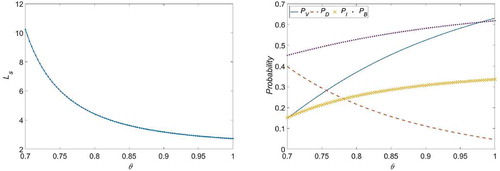
In each case, the selection of all system parameters fulfils the condition for stability. The behaviours of the performance measures for cases 1–8 are visualized in Figure 3–10, respectively. Figure 3 shows that $L_s$ increases with an increase in $\lambda$. This may be due to the fact that any increase in the arrival rate would promote an increase in the number of customers who find the server unavailable (busy or failed) and are subsequently moved into the retrial orbit. Conversely, Figures 4 and 5 show that $L_s$ decreases as ${\mu }_v$ or ${\mu }_b$ increases. In Figures 3–5, we can see that the mean arrival rate ($\lambda$) and the mean service rates (${\mu }_v$ and ${\mu }_b$) have counter effects on probabilities $P_V$, $P_D$, $P_I$, and $P_B$. We can see in Figure 6 that an increase in $\beta$ leads to (i) $L_s$ and $P_D$ decrease, and (ii) $P_V$, $P_B$ and $P_I$ increase. This can be attributed to the fact that any increase in the repair rate would increase the probability of keeping the server available or operational. In Figure 7, it is obvious that $L_s$, $P_B$ and $P_V$ decrease with an increase in the value of $\nu$. We can also see that $P_I$ increases as $\nu$ increases. Figure 8 shows that the larger is $\gamma$, the smaller are $L_s$ and $P_I$. Furthermore, any increase in $\gamma$ would lead to increases in $P_B$ and $P_V$. Thus, it is reasonable that an increase in $\gamma$ would lead to an increase in the frequency with which customers make repeated attempts to access service. Moreover, Figures 7 and 8 show that $P_D$ is insensitive to change in $\nu$ or $\gamma$. Figures 9 and 10 clearly show that (i) $L_s$ and $P_D$ decrease with an increase in $\delta$ or $\theta$, and (ii) $P_I$, $P_V$ and $P_B$ increase as $\delta$ or $\theta$ increases. Based on the figures described above, we can conclude that the behaviour of the performance measures is generally in line with our expectations.

Figure 3. Effect of $\lambda$ on $L_S$, $P_V$, $P_D$, $P_I$, and $P_B$ (case 1).

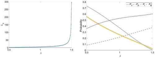
Figure 4. Effect of ${\mu }_v$ on $L_S$, $P_V$, $P_D$, $P_I$, and $P_B$ (case 2).

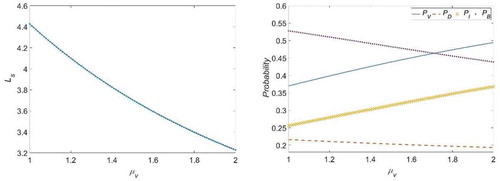
Figure 5. Effect of ${\mu }_b$ on $L_S$, $P_V$, $P_D$, $P_I$, and $P_B$ (case 3).

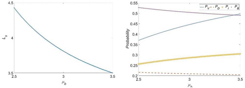
Figure 6. Effect of $\beta$ on $L_S$, $P_V$, $P_D$, $P_I$, and $P_B$ (case 4).

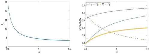
Figure 7. Effect of $\nu$ on $L_S$, $P_V$, $P_D$, $P_I$, and $P_B$ (case 5).

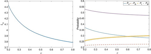
Figure 8. Effect of $\gamma$ on $L_S$, $P_V$, $P_D$, $P_I$, and $P_B$ (case 6).

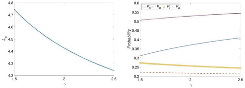
Figure 9. Effect of $\delta$ on $L_S$, $P_V$, $P_D$, $P_I$, and $P_B$ (case 7).

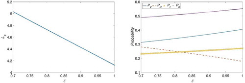
Figure 10. Effect of $\theta$ on $L_S$, $P_V$, $P_D$, $P_I$, and $P_B$ (case 8).

5. The cost model and optimization

We construct an expected cost function per unit time, in which the service rates ${\mu }_v$ and ${\mu }_b$ are decision variables. We define the cost elements as follows:

$C_h\equiv$ holding cost per unit time per customer in the system;

$C_v\equiv$ cost per unit time when the server is on vacation;

$C_b\equiv$ cost per unit time when the server is busy;

$C_1\equiv$ cost per customer served under mean service rate ${\mu }_v$;

$C_2\equiv$ cost per customer served under mean service rate ${\mu }_b$.

Based on the above definitions of the cost elements and the corresponding performance measures of the system, the expected cost function per unit time can be derived as follows:

(21) $F({\mu }_v,{\mu }_b)=C_h{L}_s+C_v{P}_V+C_b{P}_B+C_1{\mu }_v+C_2{\mu }_b,$(21)

where $L_s$, $P_V$ and $P_B$ are obtained using Equations (15), (17) and (20), respectively. In Equation (21), the first term refers to the cost incurred by customers in the system, and the last four terms denote the costs incurred by the server. Our purpose is to determine the optimal service rates $({\mu }_v^{\ast },{\mu }_b^{\ast })$ by minimizing the expected cost function shown in Equation (21), where $F({\mu }_v^{\ast },{\mu }_b^{\ast })$ represents the corresponding minimum value of the expected cost function; i.e. $F({\mu }_v^{\ast },{\mu }_b^{\ast })=\underset{{\mu }_v,{\mu }_b}{min}F({\mu }_v,{\mu }_b)$. The expected cost function is complex and rigorous, making it difficult to derive explicit expressions for the optimal service rates. We, therefore, calculate numerical solutions.

5.1. Canonical particle swarm optimization algorithm

The particle swarm optimization (PSO) algorithm introduced by Kennedy and Eberhart [38] is an efficient stochastic approach to optimizing continuous nonlinear functions. For more information on the PSO algorithm, readers are referred to [39–41]. In this study, we utilize the canonical particle swarm optimization (CPSO) algorithm presented by Carlisle and Dozier [42] to obtain numerical results for $({\mu }_v^{\ast },{\mu }_b^{\ast })$. The CPSO algorithm has been widely used by several researchers to solve optimization problems in a variety of queueing systems ([43–47]). To approximate an optimal solution for $({\mu }_v^{\ast },{\mu }_b^{\ast })$, we implement the following procedure based on the CPSO algorithm.

Step 1: Set $t=0$, the population size $M$, the upper bound of the position value $X_{max}$, and the lower bound of the position value $X_{min}$.

Step 2: The initial positions and velocities of particles are randomly generated as follows: $X_i^{(t)}=(x_{1,i}^{(t)},x_{2,i}^{(t)})$ and $V_i^{(t)}=(v_{1,i}^{(t)},v_{2,i}^{(t)})$, where $i=1,2,...,M$.

Step 3: Assess the fitness values of each particle using the expected cost function in Equation (21); i.e., $F(X_i^{(t)})=F(x_{1,i}^{(t)},x_{2,i}^{(t)})$.

Step 4: The initial position of the particle i is set to the initial personal best position of the particle i ($pbes{t}_i^{(0)}$), and the initial global best position of all particles is set to $gbest=\underset{1\le i\le N}{arg}\{minF(X_i^{(0)})\}$.

Step 5: Update the velocity of each particle using the following equation:

$v_{d,i}^{(t+1)}=\left\{\begin{array}{c}\mathrm{{\rm Y}}\left(v_{d,i}^{(t)}+c_1{r}_1(pbes{t}_i^{(t)}-x_{d,i}^{(t)})+c_2{r}_2(gbes{t}^{(t)}-x_{d,i}^{(t)})\right),X_{min}<x_{d,i}^{(t)}<X_{max},\\ 0,\mathrm{o}\mathrm{t}\mathrm{h}\mathrm{e}\mathrm{r}\mathrm{w}\mathrm{i}\mathrm{s}\mathrm{e},\end{array}\right.$

where $d=1,2$ and $i=1,2,...,M$. We generate random values for $r_1$ and $r_2$ in [0, 1]. Note that $\mathrm{{\rm Y}}=2/|2-\phi -\sqrt{{\phi }^2-4\phi }|$ is the constriction coefficient, and $\phi$ is the sum of acceleration constants $c_1$ and $c_2$; i.e. $\phi =c_1+c_2$. Moreover, $c_1$ and $c_2$ are set to 2.8 and 1.3, respectively.

Step 6: Update the position of each particle using the following equation:

$x_{d,i}^{(t+1)}=\left\{\begin{array}{c}{x}_{d,i}^{(t)}+v_{d,i}^{(t+1)},X_{min}<x_{d,i}^{(t)}+v_{d,i}^{(t+1)}<X_{max},\\ X_{max},x_{d,i}^{(t)}+v_{d,i}^{(t+1)}>X_{max},\\ X_{min},x_{d,i}^{(t)}+v_{d,i}^{(t+1)}<X_{min}.\end{array}\right.$

Step 7: Update the personal best position of particle i ($pbes{t}_i^{(t)}$) and the global best position of all particles $gbest$.

Step 8: Update the iteration counter $t=t+1$.

Step 9: Stopping criterion: If $\underset{1\le i\le M}{max}F(X_i^{(t)})-\underset{1\le j\le M}{min}F(X_j^{(t)})$ is less than tolerance $\epsilon$, then the algorithm terminates; else return to Step 5.

Step 10: Output $({\mu }_v^{\ast },{\mu }_b^{\ast })=gbest$ and $F({\mu }_v^{\ast },{\mu }_b^{\ast })$.

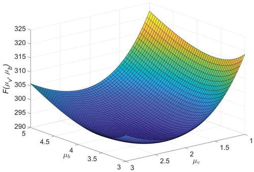
5.2. Numerical results

In the following, we present a numerical experiment to check the convexity of $F({\mu }_v,{\mu }_b)$. The graphical representation of $F({\mu }_v,{\mu }_b)$ is plotted in Figure 11 with the following parameter setting: $N=30$, $\lambda =1.0$, $\gamma =2.0$, $\beta =1.0$, $v=0.2$, $\delta =0.9$, $\theta =0.8$, $C_h=45$, $C_v=60$, $C_b=90,$ $C_1=30$, and $C_2=15$. Figure 11 shows that $F({\mu }_v,{\mu }_b)$ is convex with respect to service rates ${\mu }_b$ and ${\mu }_v$; i.e. there exists a (local) minimum in the surface of the expected cost. We find the minimum expected cost using the CPSO algorithm to approximate the optimal values for ${\mu }_b$ and ${\mu }_v$. We then explore the sensitivity of the approximate optimal service rates $({\mu }_v^{\ast },{\mu }_b^{\ast })$ with respect to various system parameters. In implementing the CPSO algorithm, we fix the upper and lower bounds of ${\mu }_b$ and ${\mu }_v$ at 0 and $10\lambda$, respectively. The population size is set to 500 ($M=500$), and the tolerance is set to 0.01 ($\epsilon ={10}^{-2}$). The results are given in Tables 1–6, wherein CPU time represents the running time (in seconds) of the algorithm.

Table 1. Optimal service rates $({\mu }_v^{\ast },{\mu }_b^{\ast })$ and the corresponding expected cost $F({\mu }_v^{\ast },{\mu }_b^{\ast })$ for different values of $\lambda$.

$\lambda$	0.5	1.0	1.5	2.0	2.5	3.0
${\mu }_v^{\ast }$	1.4932	2.1842	2.8395	3.4717	4.0449	4.3651
${\mu }_b^{\ast }$	1.5810	3.6002	6.7294	11.8441	21.2200	30.0000
$F({\mu }_v^{\ast },{\mu }_b^{\ast })$	189.796	290.395	432.258	661.191	1083.050	2301.318
Iterations	47	64	47	62	59	54
CPU time	43.091	100.785	95.806	161.140	203.165	341.029

Table 2. Optimal service rates $({\mu }_v^{\ast },{\mu }_b^{\ast })$ and the corresponding expected cost $F({\mu }_v^{\ast },{\mu }_b^{\ast })$ for different values of $\beta$.

$\beta$	0.5	0.7	0.9	1.1	1.3	1.5
${\mu }_v^{\ast }$	2.2472	2.1887	2.1820	2.1879	2.1966	2.2055
${\mu }_b^{\ast }$	6.8209	4.6189	3.8268	3.4315	3.1986	3.0465
$F({\mu }_v^{\ast },{\mu }_b^{\ast })$	448.016	335.273	299.848	283.586	274.546	268.895
Iterations	56	85	115	173	61	48
CPU time	124.829	138.64	195.984	232.822	68.648	2953.08

Table 3. Optimal service rates $({\mu }_v^{\ast },{\mu }_b^{\ast })$ and the corresponding expected cost $F({\mu }_v^{\ast },{\mu }_b^{\ast })$ for different values of $v$.

$v$	0.5	0.7	0.9	1.1	1.3	1.5
${\mu }_v^{\ast }$	1.2032	0.7135	0.2945	0	0	0
${\mu }_b^{\ast }$	3.9246	4.0103	4.0577	4.0846	4.1082	4.1260
$F({\mu }_v^{\ast },{\mu }_b^{\ast })$	274.079	265.080	257.431	250.880	245.968	242.385
Iterations	45	62	47	46	51	58
CPU time	65.869	82.761	68.052	65.692	71.943	80.614

Table 4. Optimal service rates $({\mu }_v^{\ast },{\mu }_b^{\ast })$ and the corresponding expected cost $F({\mu }_v^{\ast },{\mu }_b^{\ast })$ for different values of $\gamma$.

$\gamma$	0.5	1.0	1.5	2.0	2.5	3.0
${\mu }_v^{\ast }$	1.2349	1.8555	2.0781	2.1843	2.2437	2.2809
${\mu }_b^{\ast }$	5.1534	4.2113	3.8171	3.6002	3.4634	3.3695
$F({\mu }_v^{\ast },{\mu }_b^{\ast })$	340.251	309.048	297.049	290.395	286.118	283.128
Iterations	95	40	101	43	52	89
CPU time	135.811	50.677	136.717	59.182	70.484	118.308

Table 5. Optimal service rates $({\mu }_v^{\ast },{\mu }_b^{\ast })$ and the corresponding expected cost $F({\mu }_v^{\ast },{\mu }_b^{\ast })$ for different values of $\delta$.

$\delta$	0.3	0.4	0.5	0.6	0.7	0.8
${\mu }_v^{\ast }$	0.5793	0.8332	1.1059	1.3884	1.6637	1.9222
${\mu }_b^{\ast }$	3.8856	3.8804	3.8731	3.8562	3.8191	3.7439
$F({\mu }_v^{\ast },{\mu }_b^{\ast })$	370.612	361.847	351.046	338.241	323.665	307.700
Iterations	45	42	55	50	86	52
CPU time	86.399	73.611	94.646	78.236	125.566	74.321

Table 6. Optimal service rates $({\mu }_v^{\ast },{\mu }_b^{\ast })$ and the corresponding expected cost $F({\mu }_v^{\ast },{\mu }_b^{\ast })$ for different values of $\theta$.

$\theta$	0.55	0.6	0.7	0.8	0.9	1.0
${\mu }_v^{\ast }$	3.4578	2.8021	2.3038	2.1842	2.1680	2.1843
${\mu }_b^{\ast }$	10.0000	10.0000	5.2442	3.6002	2.8435	2.4279
$F({\mu }_v^{\ast },{\mu }_b^{\ast })$	1772.060	574.944	346.610	290.395	268.831	258.717
Iterations	44	97	65	72	59	135
CPU time	268.664	238.092	108.138	99.508	71.901	147.042

Figure 11. Expected cost $F({\mu }_v,{\mu }_b)$ for various values of ${\mu }_v$ and ${\mu }_b$.

From Table 1, we can see that ${\mu }_v^{\ast }$ and ${\mu }_b^{\ast }$ increase with an increase in $\lambda$. This can be attributed to the fact that an increase in the arrival rate would increase the probability of congestion. An increase in the service rate would decrease the congestion of the system. From Table 2, it reveals that ${\mu }_b^{\ast }$ decreases with an increase in the value of $\beta$. Table 3 shows that ${\mu }_v^{\ast }$ decreases and ${\mu }_b^{\ast }$ increases as $v$ increases. It is noted that ${\mu }_v^{\ast }$ remains at 0 even when $v$ is varied between 1.1 and 1.5. As shown in Table 4, ${\mu }_v^{\ast }$ increases and ${\mu }_b^{\ast }$ decreases with an increase in $\gamma$. In Table 5, one can see that an increase in $\delta$ causes ${\mu }_v^{\ast }$ to increase and ${\mu }_b^{\ast }$ to decrease. We can see in Table 6 that ${\mu }_v^{\ast }$ decreases when $\theta$ is varied from 0.55 to 0.9. Furthermore, increasing $\theta$ leads to a decrease in ${\mu }_b^{\ast }$. As shown in Table 1–6, $F({\mu }_v^{\ast },{\mu }_b^{\ast })$ increases with an increase in the value of $\lambda$ and decreases with an increase in any one of the parameters $\beta$, $v$, $\gamma$, $\delta$, or $\theta$. The results listed above demonstrate that system managers could optimize system costs by adjusting various system parameters. This observation provides a useful reference for decision-making.

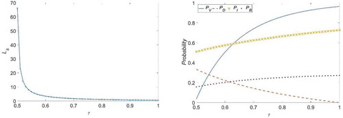
5.3. A special case and numerical comparison

The model of Do [27] is a special case of our model when $\delta =\theta =1$ (the server always starts successfully) and $N=1$ (constant retrial policy). We set $\tau =\delta =\theta$ and choose the system parameters as $N=1$, $\lambda =1.0$, $\gamma =3.0$, $\beta =3.0$, and $v=0.2$. The cost elements are identical to those used in Section 5.2. We select different values of $\tau$ to compare the numerical results with Do [27]’s model. Given the mean service rates ${\mu }_v=3.5$ and ${\mu }_b=6.5$, Figure 12 shows that the effects of $\tau$ on some performance measures. It reveals that $L_s$ and $P_D$ decrease as $\tau$ increases. This is because that when $\tau$ increases, the server is less prone to breakdowns, which leads to the smaller value of $L_S$ and $P_D$. It is also found that $P_V$, $P_I$ and $P_B$ increase with an increase in $\tau$. Table 7 shows the optimal service rates $({\mu }_v^{\ast },{\mu }_b^{\ast })$ and the corresponding expected cost $F({\mu }_v^{\ast },{\mu }_b^{\ast })$ for different values of $\tau$. From Table 7, we observe that ${\mu }_v^{\ast }$ increases and ${\mu }_b^{\ast }$ decreases as $\tau$ increases. Moreover, it is found that $F({\mu }_v^{\ast },{\mu }_b^{\ast })$ decreases with increasing values of $\tau$. Therefore, we conclude that the probability $\tau$ has an impact on the performance measures, the optimal service rates, and the minimum expected cost per unit time.

Table 7. Optimal service rates $({\mu }_v^{\ast },{\mu }_b^{\ast })$ and the corresponding expected cost $F({\mu }_v^{\ast },{\mu }_b^{\ast })$ for different values of $\tau$.

$\tau$	0.5	0.6	0.7	0.8	0.9	1.0
${\mu }_v^{\ast }$	1.9544	2.1495	2.3090	2.4291	2.5209	2.5341
${\mu }_b^{\ast }$	15.3794	6.4964	4.3709	3.4129	2.8591	2.5341
$F({\mu }_v^{\ast },{\mu }_b^{\ast })$	733.521	391.981	316.170	282.770	263.354	250.272
Iterations	63	129	80	75	81	146
CPU time	189.996	202.83	81.788	64.783	57.212	53.376

Figure 12. Effect of $\tau$ on $L_S$, $P_V$, $P_D$, $P_I$, and $P_B$.

6. Conclusions

In this paper, we analysed the M/M/1/WV retrial queue with starting failures. The proposed queueing model was described by a QBD process. We first derived the stability conditions of the model. We then used the matrix-geometric method to obtain the stationary probability distribution and developed a number of performance measures. We formulated a cost optimization problem to determine the optimal service rates $({\mu }_v^{\ast },{\mu }_b^{\ast })$ at the minimum expected cost per unit time. The CPSO algorithm was employed to obtain numerical solutions for $({\mu }_v^{\ast },{\mu }_b^{\ast })$. We also examined the effects of various system parameters on performance measures and $({\mu }_v^{\ast },{\mu }_b^{\ast })$ through numerical experiments. In future works, the arrival process could be extended to the Markovian arrival process. Another direction would be to study the proposed queueing model within scenarios involving multiple servers.

Acknowledgments

The authors thank two anonymous referees for their valuable comments on this manuscript. This work was partially supported by the Ministry of Science and Technology, Taiwan, under Grant No. MOST 107-2218-E-009-058-MY2.

Disclosure statement

No potential conflict of interest was reported by the authors.

Additional information

Funding

This work was partially supported by the Ministry of Science and Technology, Taiwan [MOST 107-2218-E-009-058-MY2].

References

- T. Yang and J.G.C. Templeton, A survey on retrial queues, Queueing Syst. 2 (1987), pp. 201–233. doi:10.1007/BF01158899
- C. Shekhar, A.A. Raina, and A. Kumar, A brief review on retrial queue: Progress in 2010–2015, Int. J. Appl. Sci. Eng. Res. 5 (2016), pp. 324–336. doi:10.6088/ijaser.05032
- J.R. Artalejo, A classified bibliography of research on retrial queues: Progress in 1990–1999, Top. 7 (1999), pp. 187–211. doi:10.1007/BF02564721
- J.R. Artalejo, Accessible bibliography on retrial queues, Math. Comput. Model. 30 (1999), pp. 1–6. doi:10.1016/j.mcm.2009.12.011
- J.R. Artalejo, Accessible bibliography on retrial queues: Progress in 2000–2009, Math. Comput. Model. 51 (2010), pp. 1071–1081. doi:10.1016/j.mcm.2009.12.011
- G.I. Falin and J.G.C. Templeton, Retrial Queues, Chapman and Hall, London, 1997.
- J.R. Artalejo and A. Gomez-Corral, Retrial Queueing Systems: A Computational Approach, Springer-Verlag, Berlin, Heidelberg, 2008.
- N.P. Sherman and J.P. Kharoufeh, An M/M/1 retrial queue with unreliable server, Oper. Res. Lett. 34 (2006), pp. 697–705. doi:10.1016/j.orl.2005.11.003
- G. Falin, An M/G/1 retrial queue with an unreliable server and general repair times, Perform. Eval. 67 (2010), pp. 569–582. doi:10.1016/j.peva.2010.01.007
- G. Choudhury and J.-C. Ke, An unreliable retrial queue with delaying repair and general retrial times under Bernoulli vacation schedule, Appl. Math. Comput. 230 (2014), pp. 436–450. doi:10.1016/j.amc.2013.12.108
- F.-M. Chang, T.-H. Liu, and J.-C. Ke, On an unreliable-server retrial queue with customer feedback and impatience, Appl. Math. Model. 55 (2018), pp. 171–182. doi:10.1016/j.apm.2017.10.025
- T. Yang and H. Li, The M/G/1 retrial queue with the server subject to starting failures, Queueing Syst. 16 (1994), pp. 83–96. doi:10.1007/BF01158950
- B.K. Kumar, S.P. Madheswari, and A. Vijayakumar, The M/G/1 retrial queue with feedback and starting failures, Appl. Math. Model. 26 (2002), pp. 1057–1075. doi:10.1016/S0307-904X(02)00061-6
- J. Wang and Q. Zhao, A discrete-time Geo/G/1 retrial queue with starting failures and second optional service, Comput. Math. Appl. 53 (2007), pp. 115–127. doi:10.1016/j.camwa.2006.10.024
- I. Atencia, I. Fortes, and S. Sánchez, A discrete-time retrial queueing system with starting failures, Bernoulli feedback and general retrial times, Comput. Ind. Eng. 57 (2009), pp. 1291–1299. doi:10.1016/j.cie.2009.06.011
- J. Wang and P.-F. Zhou, A batch arrival retrial queue with starting failures, feedback and admission control, J. Syst. Sci. Syst. Eng. 19 (2010), pp. 306–320. doi:10.1007/s11518-010-5140-z
- D.-Y. Yang, J.-C. Ke, and C.-H. Wu, The multi-server retrial system with Bernoulli feedback and starting failures, Int. J. Comput. Math. 92 (2015), pp. 954–969. doi:10.1080/00207160.2014.932908
- J.-C. Ke, T.-H. Liu, and D.-Y. Yang, Retrial queues with starting failure and service interruption, IET Commun. 12 (2018), pp. 1431–1437. doi:10.1049/iet-com.2017.0820
- Y. Levy and U. Yechiali, Utilization of idle time in an M/G/1 queueing system, Manage. Sci. 22 (1975), pp. 202–211. doi:10.1287/mnsc.22.2.202
- B.T. Doshi, Queueing systems with vacations—a survey, Queueing Syst. 1 (1986), pp. 29–66. doi:10.1007/BF01149327
- H. Takagi, Queueing Analysis: A Foundation of Performance Evaluation, Vol. 1, North-Holland, Amsterdam, 1991.
- N.-S. Tian and Z.G. Zhang, Vacation Queueing Models: Theory and Applications, Springer-Verlag, New York, 2006.
- J.-C. Ke, C.-H. Wu, and Z.-G. Zhang, Recent developments in vacation queueing models: a short survey, Int. J. Oper. Res. 7 (2010), pp. 3–8.
- L.D. Servi and S.G. Finn, M/M/1 queues with working vacations (M/M/1/WV), Perform. Eval. 50 (2002), pp. 41–52. doi:10.1016/S0166-5316(02)00057-3
- N.-S. Tian, J.-H. Li, and Z.G. Zhang, Matrix analytic method and working vacation queues—a survey, Int. J. Inf. Manage. Sci. 20 (2009), pp. 603–633.
- V.M. Chandrasekaran, K. Indhira, M.C. Saravanarajan, and P. Rajadurai, A survey on working vacation queueing models, Int. J. Pure Appl. Math. 106 (2016), pp. 33–41. doi:10.12732/ijpam.v106i6.5
- T.V. Do, M/M/1 retrial queue with working vacations, Acta Inform. 47 (2010), pp. 67–75. doi:10.1007/s00236-009-0110-y
- T. Li, Z. Wang, and Z. Liu, Geo/Geo/1 retrial queue with working vacations and vacation interruption, J. Appl. Math. Computing. 39 (2012), pp. 131–143. doi:10.1007/s12190-011-0516-x
- Z. Liu and Y. Song, Geo/Geo/1 retrial queue with non-persistent customers and working vacations, J. Appl. Math. Computing. 42 (2013), pp. 103–115. doi:10.1007/s12190-012-0623-3
- L. Tao, Z. Liu, and Z. Wang, M/M/1 retrial queue with collisions and working vacation interruption under N-policy, Rairo-Oper. Res. 46 (2012), pp. 355–371. doi:10.1051/ro/2012022
- T. Li, L. Zhang, and S. Gao, Performance of an M/M/1 retrial queue with working vacation interruption and classical retrial policy, Adv. Oper. Res. (2016), Article ID 4538031, PP. 9. doi:10.1155/2016/4538031.
- D. Arivudainambi, P. Godhandaraman, and P. Rajadurai, Performance analysis of a single server retrial queue with working vacation, Opsearch. 51 (2014), pp. 434–462. doi:10.1007/s12597-013-0154-1.
- S. Gao, J. Wang, and W.W. Li, An M/G/1 retrial queue with general retrial times, working vacations and vacation interruption, Asia Pac. J. Oper. Res. 31 (2014), pp. 25. doi:10.1142/S0217595914400065.
- T. Li, L. Zhang, and S. Gao, An M/G/1 retrial queue with balking customers and Bernoulli working vacation interruption, Qual. Technol. Quant. Manag. 16 (2019), pp. 511–530. doi:10.1080/16843703.2018.1480264
- N.H. Do, T.V. Do, and A. Melikov, Equilibrium customer behavior in the M/M/1 retrial queue with working vacations and a constant retrial rate, Oper. Res. Int. J. (2018). doi:10.1007/s12351-017-0369-7.
- J.S.H. Van Leeuwaarden, M.S. Squillante, and E.M.M. Winands, Quasi-birth-and-death processes, lattice path counting, and hypergeometric functions, J. Appl. Probab. 46 (2009), pp. 507–520. doi:10.1239/jap/1245676103
- M. Neuts, Matrix-Geometric Solutions in Stochastic Models, Johns Hopkins University Press, Baltimore, 1981.
- J. Kennedy and R. Eberhart, PSO optimization. In Proceedings of the IEEE international conference on Neural Networks, IEEE service center, Piscataway, NJ, pp. 1942–1948, 1995.
- Y. Shi and R. Eberhart, A modified particle swarm optimizer, In Proceedings of the IEEE International Conference on Evolutionary Computation, Anchorage, AK, USA, 1998, pp.69–73.
- J. Robinson and Y. Rahmat-Samii, Particle swarm optimization in electromagnetics, IEEE Trans. Antennas Propag. 52 (2004), pp. 397–407. doi:10.1109/TAP.2004.823969
- R. Poli, J. Kennedy, and T. Blackwell, Particle swarm optimization, Swarm Intell. 1 (2007), pp. 33–57. doi:10.1007/s11721-007-0002-0
- A. Carlisle and G. Dozier, An off-the-shelf PSO, In Proceeding of the workshop on particle swarm optimization, Purdue School of Engineering and Technology, Indianapolis, 2001.
- X. Zhang, J. Wang, and T.V. Do, Threshold properties of the M/M/1 queue under T-policy with applications, Appl. Math. Comput. 261 (2015), pp. 284–301. doi:10.1016/j.amc.2015.03.109
- X. Zhang, J. Wang, and Q. Ma, Optimal design for a retrial queueing system with state-dependent service rate, J. Syst. Sci. Complex. 30 (2017), pp. 883–900. doi:10.1007/s11424-017-5097-9
- Y. Zhang and J. Wang, Equilibrium pricing in an M/G/1 retrial queue with reserved idle time and setup time, Appl. Math. Model. 49 (2017), pp. 514–530. doi:10.1016/j.apm.2017.05.017
- J. Wang, X. Zhang, and P. Huang, Strategic behavior and social optimization in a constant retrial queue with the N-policy, Eur. J. Oper. Res. 256 (2017), pp. 841–849. doi:10.1016/j.ejor.2016.06.034
- K.-H. Wang, J. Wang, C.-D. Liou, and X. Zhang, Particle swarm optimization to the retrial machine repair problem with working breakdowns under the N policy, Queueing Mod, Serv. Manage 2 (2019), pp. 61–81.