Nonlinear modeling and performance analysis of a closed-loop supply chain in the presence of stochastic noise

ABSTRACT

We study four-echelon supply chains consisting of manufacturer, wholesaler, retailer and customer with recovery center as hybrid recycling channels. In order to gain a larger market share, the retailer often takes the sales as a decision-making variable. For this purpose, in this supply chain, the retailer limits the forecast of market demand in future periods with expected logic. It also manages demand by leveraging prices and choosing market. In this paper, first, we investigate the state-space model of this supply chain system and examine the effect of complex dynamic and stochastic noise on the bullwhip effect. We analytically prove that this factor leads to the bullwhip effect. So, first, we filtered the information between nodes with extended Kalman filter after which we regulated the destructive effects of the bullwhip phenomenon by designing a non-linear quadratic Gaussian optimal controller. Eventually, the simulation results indicate the efficiency of the proposed method.

KEYWORDS:

• Non-linear supply chain
• EKF
• LQG
• hybrid recycling channels
• bullwhip effect
• sales game

1. Introduction

The concept of supply chain management (SCM) is becoming more popular today, given the progressive global competition in the global marketplace [1]. SCM may be defined as a set of relationships between suppliers, manufacturers, distributors and retailers, which transforms the raw materials to the end products [2]. Modelling and controlling such systems involve taking all commercial components into account in this complexity [1]. SCM has recently attracted a great deal of attention among engineers in the processing system [3]. The tendency of orders to increase in diversity as a supply chain move is commonly known as the bullwhip effect. Dejonckheere [4] initiated the analysis of this variance amplification phenomenon, whose work has inspired many authors to develop business games to demonstrate the bullwhip effect.

Due to global population increasing, the social economy developing and people’s living standard improving, the existing natural resources are not sufficient to meet people’s needs where earth’s ecosystems are facing progressive threat [5]. As a result, many enterprises are actively planning their supply chain structures in order to better handle both the forward flow and the reverse flow of product [6]. In real life, some manufacturers entrust a third-party recovery provider to be responsible for the task of recycling business. So, the recovery process can be completed by the manufacturer and third-party recovery provider simultaneously which is called hybrid recycling channels.

Since demand forecasting is one of the main reasons for the effect of the bullwhip effect, many scholars seek to develop prediction methods and inventory control systems to fulfil the demand during lead time services. Chen et al. [7] quantified the effects of the bullwhip on a simple and two-stage supply chain, including a retailer and a producer, using the moving average and exponential smoothing method.

In production systems for ordering, the manufacturer must be able to coordinate himself with the demand of different markets and deliver the product at the desired times with the right and desirable quality. In most of the production planning models that have been reviewed so far, the demand for products in different periods of planning horizon is already set which becomes an uncontrollable factor outside of the production system into the model. Note that regardless of the conditions of competitive markets and demand growth, and despite limited production capacity, it is not mandatory to meet all the demands of the manufacturer. Therefore, the manufacturer must be able to control the level of demand by applying leverage. Two convenient levers in demand management include pricing and selecting the target market. In real problems, despite the diversity and competitiveness of manufacturing companies, the customer has the right to choose his product from similar products by different manufacturers [8].

Selection of inventory management policies is recognized as an important factor in controlling supply chain costs. One of the important and efficient approaches to improving the dynamics of the supply chain is the use of control theory methods [9]. As an introduction to the first applications of linear control theory, we refer the reader to Franklin et al. [10], to Nise [11] and to Benett [12] for a brief overview of its historic background. In an inventory management field, linear control method was first applied by Simon [13] and Vassion [14], where Simon took into account the continuous form of time for studying the steady-state behaviour of an existing system. Vassion investigated a discrete time display to apply an order based on the customer’s current order. Meyer and Groover [15] along with Burns and Sivazlian [16] were the first to investigate linear control methods to analyse multi-echelon problems. In recent years, linear control methods have been used to develop existing policies and investigate the bullwhip effects. John et al. [17] introduced the APIOBPCS (Automatic Pipeline, inventory and order-based production control system) inventory policy which bases orders on a demand anticipation, the error between target and actual inventory, and the error between target and actual effort in progress. Dejonckheere et al. [4] introduced an order increase induced by order-up-to policies and the APIOBPCS method. Dejonckheere et al. [18] investigated our work by analysing the effect of sharing data to enhance order changes. In addition to order variability, Disney and Towill [19] probed the inventory amplification induced by an APIOBPCS-related inventory methods.

Berrin Agaran et al. [1] introduced modern control theory and Linear Quadratic Gauss controller to regulating bullwhip effect phenomenon. Their work provided the opportunity to extend the modelling and control work to non-linear, time-varying, stochastic, adaptive and large-scale systems. Pin et al. [3] reduced bullwhip in supply chain via z-transform analysis. Ignaciuk et al. [20] designed an optimal strategy with Linear Quadratic Integretorcontroller in supply chain to mitigate demand variability. Chandra et al. [21] designed a controllable, observable and stable supply chain system representation of a generalized order-up-to policy. Further, Dongfei et al. [22] quantified and mitigated the bullwhip in a benchmark supply chain by extending prediction self-adaptive control.

For hybrid recycling channels, Li et al. [23] analysed the stable operation of a closed-loop supply chain with mixed recycling channels using game theory. Yi and Liang [24] constructed three hybrid recycling methods of the product remanufacturing closed-loop supply chain under premium and penalty mechanisms. One of the key issues was the selection of a suitable channel pattern among the three hybrid gathering channels [25]. Other researchers [26,27] attempted to reduce the fluctuation resulting from the complexity of hybrid recycling through analysing robust stability of closed-loop forms. Elsewhere, Zhang et al. [28] employed fuzzy control method to control the bullwhip effect in uncertain closed-loop supply chains with hybrid recycling channels [28]. Zheng et al. managed to restrain bullwhip effect by considering the uncertainties in the closed-loop supply chain system and fuzzy control method (Takagi-Sugeno). Their method not only restrained the bullwhip effect but also caused the supply chain to retain robust stability.

The first step in regulating the bullwhip effect is measuring this phenomenon. Goodarzi et al. [29] measured the bullwhip effect using network data envelopment analysis. They introduced a new mathematical model to measure the bullwhip effect and presented a non-radial WPF-DEA model with a network structure. In Kannan Govindan et al.'s [30] research, planning decisions, network combination, samples and position related to SCM were considered. They also explored the existing optimization materials for dealing with uncertainty, such as recourse-based stochastic programming, risk-averse stochastic programming, robust optimization and fuzzy mathematical programming in the qualification of mathematical modelling and solution approaches.

SMC is useful in reducing inventory oscillation. In Ignaciuk et al.'s [32]research, LQ optimal sliding mode supply policy was developed for periodic review inventory systems. Piotr Levniewski et al. [33] applied the control-theoretic approach to design a new replenishment law for supply chain systems with perishable inventory. They represented a Bartoszewicz et al.'s [34] proposed sliding mode control of inventory management systems with a bounded batch size. Their proposed law for such systems ensured full consent of the ambivalent consumers’ demand while adhering to state and input constraints. sliding mode control and selected its parameters to minimize a quadratic quality criterion. The control method proposed in their research ensured bounded orders, guaranteed full consumers’ demand satisfaction, and decreased the risk of exceeding the warehouse capacity

Also, Wandong et al. [34] attempted to mitigate the bullwhip phenomenon in supply chains with sales game and consumer returns using chaos theory. They studied a supply chain system consisting of one manufacturer and two retailers including a traditional retailer and an online retailer. It supposed bounded rational expectation to anticipate the future demand in the sale game system with weak noise. They found that high return rates will reduce the profit of both retailers and the adjustment speed of the bounded rational sales expectation. In this work, the demand was as regarded as an uncontrollable input, but Torabi et al. [35] in their research attempted to consider demand as a controllable factor and decision-making variable. They presented an innovative algorithm in an NP (Network Petri)-hard model to minimize linear target.

The rest of the paper is organized as follows. In Section 2, we develop the dynamic model of supply chain with hybrid recycling channel and sales game. In Section 3, the model is analysed and in Section 4, we design LQG optimal control to restrain the bullwhip effect. Numerical simulations are provided based on the proposed method in Section 5. Finally, the conclusions of the paper are discussed in Section 6.

2. Problem formulation

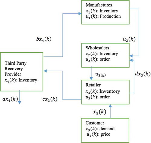
We study a supply chain model with four levels consisting of one factory, wholesaler, retailer and customer including the recovery center as hybrid recycling channel of an inventory system. The supply chain designed is intended to be controllable. Information between the nodes is visible. For this purpose, it is assumed that the nodes share their information throughout the chain.

Our target is to provide a sustainable model of fluctuation while modifying the bullwhip effect and pursuing a specific index. To achieve the desired performance, in this model, the retailer can return some of its inventory to the wholesaler for any reason. The recovery center focuses on incoming products, to return damaged product to the factory or deliver it to the retailer after recovery. Indeed, the customer is not directly connected to the recovery center. Note that designed supply chain system is discrete and time-invariant.

As mentioned earlier, it is assumed that all levels share their information, and thus all state variables are measurable.

Retailers tend to adopt some sales promotion strategies to claim a larger market share and profits. For example, they usually use advertising, gifts and other methods to stimulate consumers’ willingness to buy more, in order to achieve the goal of improving market demand for their products. We operate on the assumption that retailers make a reasonable decision to determine their sales volume. The retailer is familiar with market conditions and can easily obtain the current demand information for its products in a timely manner. Also, the retailer uses a limited logical expectation to use a sales game to predict sales volume (demand forecast) for the next period.

It is assumed that order-to-inventory policies are used by retailers, based on the current and anticipated demand for the future. Suppose that the retailers determine forecasted demand in the next period with limited rationality [31], which based on an estimated partial margin of profit for the current period. This means that the retailer will reduce its sales volume forecast for the next period if the current marginal profit is negative. The retailer will maintain its sales volume if the current marginal profit is zero; otherwise, the retailer will increase the sales volume in the next period. The inverse demand function ($k$) can be written as [36]:

(1) $k=p-qD$(1)

where the parameter p represents the acceptable price ceiling of the product for the retailer, the parameter $q$ denotes the relationship between prices and sales and $D$ is the customer demand. We can earn the profit of the retailer as follows:

(2) $\pi =D\left(p-qD\right)$(2)

The marginal profit of the retailer can be estimated by Equation (3):

(3) $\frac{\mathrm{\partial }\pi }{\mathrm{\partial }D}=p-2qD$(3)

When a retailer takes a sales game, they will consider some of the available sales information marginally. If the marginal profit is greater than zero, the retailer can increase sales based on the current sales volume. The retailers can give the forecast demand for the next period according to the bounded rational expectation:

(4) $\bar{D}=D+\alpha D\left(p-2qD\right)$(4)

The parameter $\alpha$ in Equation (4) represents the retailer adjustment speed. The value of this parameter depends on the enthusiasm of the retailer’s profit seeking. By taking the retailer demand as a state variable, the demand forecasting model with random disturbance is as follows:

(5) $x_5\left(k+1\right)=x_5\left(k\right)+\alpha x_5\left(k\right)\left(p-2q{x}_5\left(k\right)\right)$(5)

The control variable $u_4\left(\mathrm{k}\right)$ is the price (surplus penalty on the price of the product) to control the demand, which is utilized in the demand forecasting equation:

(6) $x_5\left(k+1\right)=x_5\left(k\right)+\alpha x_5\left(k\right)\left(p-2q{x}_5\left(k\right)-\theta \right)-u_4\left(k\right)$(6)

The recovery provider as a recycling channel receives defective goods and applies rebuilding measures. So, they return the repaired goods to the customer while returning the part of the goods that cannot be repaired to the factory. Equation (7) indicates the inventory position for the recovery center:

(7) $x_4\left(k+1\right)=x_4\left(k\right)+c{x}_3\left(k\right)-a{x}_4\left(k\right)-b{x}_4\left(k\right)$(7)

In step $k$, after forecasting demand, the retailer regulates his stock by sending order to the wholesaler. In this way, the retailers send some of his inventory to the recovery center and the wholesaler. The retailer inventory in step $k+1$ is obtained from Equation (8):

(8) $x_3\left(k+1\right)=x_3\left(k\right)+u_3\left(k\right)-d{x}_3\left(k\right)-c{x}_3\left(k\right)-x_5\left(k\right)$(8)

After preparing the retailer order by the wholesaler, the wholesaler will send the order to set up his inventory:

(9) $x_2\left(k+1\right)=x_2\left(k\right)+u_2\left(k\right)+d{x}_3\left(k\right)-u_3\left(k\right)$(9)

Equation (10) shows the factory inventory at period $k+1$.

(10) $x_1\left(k+1\right)=x_1\left(k\right)+u_1\left(k\right)+b{x}_4\left(k\right)-u_2\left(k\right)$(10)

As shown in Figure 1, there are many certain factors in the internal and external systems. This parameter may cause changes in the manufacturer’s inventory and retailer’s inventory. The non-linear supply chain with sales games and hybrid recycling channels is as follows:

$x_1\left(k+1\right)=x_1\left(k\right)+u_1\left(k\right)+b{x}_4\left(k\right)-u_2\left(k\right)$

$x_2\left(k+1\right)=x_2\left(k\right)+u_2\left(k\right)+d{x}_3\left(k\right)-u_3\left(k\right)$

(11) $x_3\left(k+1\right)=x_3\left(k\right)+u_3\left(k\right)-d{x}_3\left(k\right)-c{x}_3\left(k\right)-x_5\left(k\right)$(11)

$x_4\left(k+1\right)=x_4\left(k\right)+c{x}_3\left(k\right)-a{x}_4\left(k\right)-b{x}_4\left(k\right)$

$x_5\left(k+1\right)=x_5\left(k\right)+\alpha x_5\left(k\right)\left(p-2q{x}_5\left(k\right)-\theta \right)+u_4\left(k\right)$

$y_1\left(k+1\right)=x_1\left(k+1\right)$

Figure 1. The supply chain system with hybrid recycling channel and sales game.

$y_2\left(k+1\right)=x_2\left(k+1\right)$

$y_3\left(k+1\right)=x_3\left(k+1\right)$

$y_4\left(k+1\right)=x_4\left(k+1\right)$

$y_5\left(k+1\right)=x_5\left(k+1\right)$

$a+b=1$

$c+d\le 1$

Table 1 reports the operations management-related variables and parameters of the proposed non-linear supply chain model.

Table 1. Notations.

$x_1\left(k\right)$	Manufacturer inventory
$x_2\left(k\right)$	Wholesaler inventory
$x_3\left(k\right)$	Retailer inventory
$x_4\left(k\right)$	Recovery provider inventory
$x_5\left(k\right)$	Customer demand
$u_1\left(k\right)$	Production
$u_2\left(k\right)$	Wholesaler order
$u_3\left(k\right)$	Retailer order
$u_4\left(k\right)$	Price as penalty
$a$	Disposal rate
$b$	Remanufacturing rate
$c$	Recycling rate
$d$	Return rate
$p$	Acceptable price ceiling of the product for the retailer
$q$	The order quantity of retailer
$\theta$	The impact factor of return rate on the price
$\alpha$	The retailer adjustment speed

3. Main results

In this paper, we first linearize the supply chain to test the effects of system complexity and stochastic noise on the bullwhip effect. Suppose that $X=\left(x_1^{\ast }\left(k\right),x_2^{\ast }\left(k\right),x_3^{\ast }\left(k\right),x_4^{\ast }\left(k\right),x_5^{\ast }\left(k\right)\right)$ and $U=\left(u_1^{\ast }\left(k\right),u_2^{\ast }\left(k\right),u_3^{\ast }\left(k\right),u_4^{\ast }\left(k\right)\right)$ are equilibrium points for a non-linear system. Through Taylor series, we can write:

$x_1\left(k+1\right)=x_1\left(k\right)+b{x}_4\left(k\right)+u_1\left(k\right)-u_2\left(k\right)$

$x_2\left(k+1\right)=x_2\left(k\right)+d{x}_3\left(k\right)+u_2\left(k\right)-u_3\left(k\right)$

(12) $x_3\left(k+1\right)=\left(1-c-d\right)x_3\left(k\right)-x_5\left(k\right)+u_3\left(k\right)$(12)

$x_4\left(k+1\right)=c{x}_3\left(k\right)$

$x_5\left(k+1\right)=\left(1+\alpha p-4\alpha q{x}_5^{\ast }\left(k\right)\right)x_5\left(k\right)-u_4\left(k\right)$

If we suppose $x_5^{\ast }\left(k\right)=h,$then by applying z transfer, we can write:

$X_1\left(z\right)=\frac{1}{z-1}\left[b{X}_4\left(z\right)+U_1\left(z\right)-U_2\left(z\right)\right]$

$X_2\left(z\right)=\frac{1}{z-1}\left[d{X}_3\left(z\right)+U_2\left(z\right)-U_3\left(z\right)\right]$

(13) $X_3\left(z\right)=\frac{1}{z-1+c+d}\left[-X_5\left(z\right)+U_3\left(z\right)\right]$(13)

$X_4\left(z\right)=\frac{1}{z}\left[c{X}_3\left(z\right)\right]$

$X_5\left(z\right)=\frac{1}{z-1-\alpha p-4\alpha qh}\left[-U_4\left(z\right)\right]$

Then,

$U_1\left(z\right)=\left(z-1\right)X_1\left(z\right)+\left(z-1\right)X_2\left(z\right)-\left(z-1+c\right)X_3\left(z\right)-b{X}_4\left(z\right)+X_5\left(z\right)U_2\left(z\right)=\left(z-1\right)X_2\left(z\right)+\left(z-1+c\right)X_3\left(z\right)+X_5\left(z\right)$

$U_3\left(z\right)=\left(z-1+c+d\right)X_3\left(z\right)+X_5\left(z\right)$

$U_4\left(z\right)=-\left(z-1-\alpha p-4\alpha qh\right)X_5\left(z\right)$

3.1. Complexity dynamic effect on the bullwhip phenomenon

To investigate the effect of various factors on the bullwhip phenomenon, we use frequency response for every node. The transfer function in the downstream node (retailer) is as follows:

$\frac{U_3\left(z\right)}{X_5\left(z\right)}=\left(z-1+c+d\right)\frac{X_3\left(z\right)}{X_5\left(z\right)}+1$

In the case of aggressive demand (as ordering), by assuming a fixed stock for the retailer, we obtain:

(14) $\left|\frac{U_3\left(z\right)}{X_5\left(z\right)}\right|=1$(14)

Hence, in this case, the bullwhip effect does not hold.

If the downstream node sends his order via demand forecasting strategy, then we can obtain Equation (15):

(15) $U_j\left(z\right)=k_j\left(S_j\left(z\right)-X_j\left(z\right)\right),j=1,2,3$(15)

where $S_j\left(z\right)$ is the set point of inventory position at node j and $k_j$ represents the gain of proportional controller [3].

(16) $U_3\left(z\right)=k_3\left(S_3\left(z\right)-X_3\left(z\right)\right)=k\left(L{X}_5\left(z\right)-X_3\left(z\right)\right)$(16)

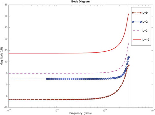
In Equation (16), $L$ is the lead time. Using Equation (13), Equation (16) becomes:

(17) $\frac{U_3\left(z\right)}{X_5\left(z\right)}=\frac{k\left(1+L\left(z-1+c+d\right)\right)}{\left(z-1+c+d+k\right)\left(z-1+c+d\right)}$(17)

The bullwhip effect can happen, if the magnitude of the transfer function in the bode diagram becomes larger than zero. The simulation results show that complex and non-linear dynamics lead to the bullwhip effect.

Figure 2 displays that when supply chain becomes complex by forecasting demand strategy and the retailer sends his order accordingly, the bullwhip effect happens. In this case, with prolongation of the lead time, the magnitude of bullwhip effect increases. Consequently, the lead time has a direct relationship with the bullwhip effect [37].

Figure 2. Frequency responses of $\frac{{\mathrm{U}}_3\left(\mathrm{z}\right)}{X_5\left(z\right)}$ in the case of complexity dynamic for various lead time.

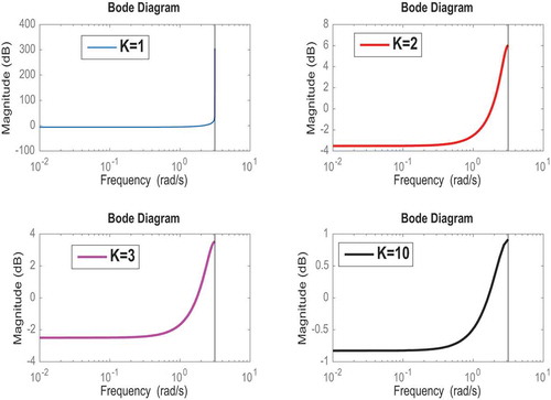
Note that the gain in ordering policy has no direct relationship with the bullwhip effect. We show that from $k=1$ until $k=2$, the magnitude of the bullwhip effect increases. However, from $k=3$ until $k=10$, the magnitude of the bullwhip effect diminishes (Figure 3).

Figure 3. Frequency responses of $\frac{{\mathrm{U}}_3\left(\mathrm{z}\right)}{X_5\left(z\right)}$ in the case of complexity dynamic for various gain.

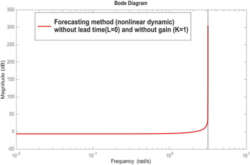
As seen in Figure 4, without any lead time and proportional gain, inevitably the bullwhip effect does not happen. In other words, if supply chain dynamics becomes complex (non-linear), then the bullwhip effect does not occur.

Figure 4. Frequency responses of $\frac{{\mathrm{U}}_3\left(\mathrm{z}\right)}{X_5\left(z\right)}$ in the case of complexity without any lead time and gain.

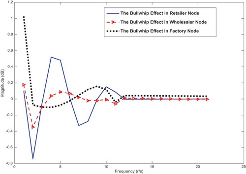
In the above, we found that non-linear dynamics leads to the bullwhip effect in downstream nodes. Subsequently, we probe these matters in upstream nodes and compare the magnitude of the bullwhip effect for downstream and upstream nodes.

Figure 5 shows the magnitude of the bullwhip effect for retailer node, wholesaler node and factory node. As seen, the bullwhip effect arising from non-linear dynamics decreases in the wholesaler node. However, this phenomenon reaches its maximum in the upstream node (factory). Therefore, we can say that it increases non uniformly.

Figure 5. The magnitude ratio of transfer function for all nodes.

3.2. Stochastic noise effect on the bullwhip phenomenon

We intend to indicate that the stochastic noisy information in the chain leads to the bullwhip effect. In this case, the supply chain with stochastic noise becomes:

$x_1\left(k+1\right)=x_1\left(k\right)+b{x}_4\left(k\right)+u_1\left(k\right)-u_2\left(k\right)+w\left(k\right)$

$x_2\left(k+1\right)=x_2\left(k\right)+d{x}_3\left(k\right)+u_2\left(k\right)-u_3\left(k\right)+w\left(k\right)$

(18) $x_3\left(k+1\right)=\left(1-c-d\right)x_3\left(k\right)-x_5\left(k\right)+u_3\left(k\right)+w\left(k\right)$(18)

$x_4\left(k+1\right)=c{x}_3\left(k\right)+w\left(k\right)$

$x_5\left(k+1\right)=\left(1+\alpha p-4\alpha qh\right)x_5\left(k\right)-u_4\left(k\right)+w\left(k\right)$

$y_1\left(k+1\right)=x_1\left(k+1\right)+v_1\left(k\right)$

$y_2\left(k+1\right)=x_2\left(k+1\right)+v_2\left(k\right)$

$y_3\left(k+1\right)=x_3\left(k+1\right)+v_3\left(k\right)$

$y_4\left(k+1\right)=x_4\left(k+1\right)+v_4\left(k\right)$

$y_5\left(k+1\right)=x_5\left(k+1\right)+v_5\left(k\right)$

where $w\left(k\right)$ is the process noise and $V\left(k\right)$ is the measurement noise vector, while usually assuming normal white noise.

We use the command ‘cra’ in MATLAB software to simulate the transfer function behaviour in the case of existence of the stochastic noise. Figure 6 indicates that the stochastic noise is one of the factors that creates the bullwhip effect. We simulated the impulse response of open-loop supply chain in four cases of stochastic noise: without noise, large variance noise ($Q_w=10,R_w=10eye\left(3\right)$), medium variance noise ($Q_w=1,R_w=1eye\left(3\right)$) and low variance noise $\left(Q_w=0.1,R_w=0.1eye\left(3\right)\right);$ where $Q_w$ and $R_w$ denote the covariance of process and measurement noise.

Figure 6. Frequency responses of $\frac{U_3\left(z\right)}{X_5\left(z\right)}$ for various variance noise (process and measurement noise).

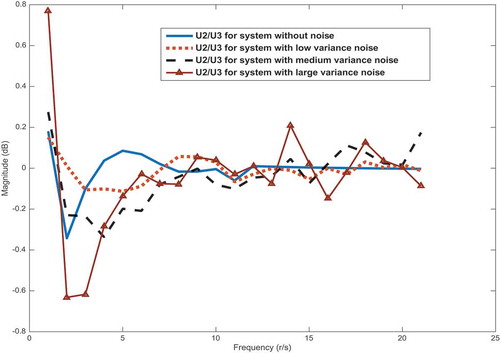
The results indicate (Figure 7) that the supply chain without noise loses its bullwhip effect form after a short period of time. Indeed, there is no bullwhip effect in the absence of noise. However, with the addition of noises to the system, the bullwhip effect appears, which is a direct relationship. As the noise increases, the bullwhip effect also grows. In general, we conclude that stochastic noise is a vital threat for the supply chain efficiency due to the information noise in modelling, engineering and statistics.

Figure 7. Frequency responses of $\frac{U_j\left(z\right)}{U_{j+1}\left(z\right)}$ for all nodes with same variance noise.

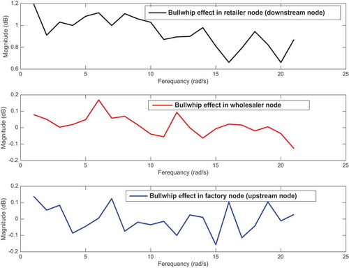
In the above, we revealed that the stochastic noise leads to the bullwhip effect in downstream nodes. Next, we probe this matter in upstream nodes and compare the magnitude of the bullwhip effect for downstream and upstream nodes.

The size of the bullwhip effect occurring by non-linear dynamics is not necessarily a bullish trend. On the contrary, the bullwhip effect generated by stochastic noise increases dramatically throughout the chain. Therefore, providing guidelines for adjusting the bullwhip effect on the supply chain with stochastic noise is important. This phenomenon can lead to a catastrophe in other noisy supply chains. Note that control theory is a powerful method for solving these problems.

4. Proposed method to mitigate the bullwhip effect

In the previous section, we proved that noisy information in the supply chain is very dangerous, as this phenomenon can lead to a catastrophe in supply chains. Therefore, filtering the information is the first attempt in regulating the bullwhip effect. One of the optimal methods to reducing the noise effect is Kalman filter (KF). One of the objectives of the optimal controller design is speed, as it is important for the simultaneous design of the controller. High speed can be achieved with great gain which causes greater sensitivity for the system in the presence of noise. The KF is indeed the state observer, with the difference in the optimal compromise between minimizing the error and reducing the effects of noise (speed of controller and minimized sensitivity to the stochastic noise). The proposed supply chain is complex and non-linear dynamic. So, we use extended Kalman filter (EKF). By filtering the information from the beginning of the chain (demand) to the end (the information received by the factory) of the chain, EKF reduces one of the most destructive factors in the supply chain.

The EKF [38] extends the scope of KF to non-linear optimal filtering problems by forming a Gaussian approximation to the joint distribution of state $x$ and measuring $y$ using a Taylor series based on transformation. The filtering model (EKF) for the suggested non-linear supply chain in Equation (11) (without inputs) to estimate the state variable is as follows:

(19) $X\left(k+1\right)=f\left(\left(k\right),k\right)+w\left(k\right)$(19)

$Y\left(k+1\right)=h\left(X\left(k\right),k\right)+V\left(k\right)$

where $X\left(k\right)\in R^n$ is the state vector, $Y\left(k\right)\in R^n$ shows the measurement vector, $w\left(k\right)\sim N\left(0,Q_w\right)$ is the process noise, $v\left(k\right)\sim N\left(0,R_w\right)$ is the measurement noise, f denotes the (possibly non-linear) dynamic model function and h represents the (again possibly non-linear) measurement model function. The first-order EKFs approximates the distribution of state $x\left(k\right)$ given the observations $y\left(1:k\right)$:

(20) $p\left(x\left(k+1\right)|y\left(1:k+1\right)\right)\approx N(x\left(k+1\right)|m\left(k+1\right),P\left(k+1\right))$(20)

As with KF, the EKF is also separated into two steps. The steps for the first-order EKF are as follows:

Prediction step is:

(21) $m^{-}\left(k+1\right)=f\left(m\left(k\right),k\right)$(21)

$p^{-}\left(k+1\right)=F_x\left(m\left(k\right),k\right)P\left(k\right)F_x^T\left(m\left(k\right),k\right)+Q_w$

Also, the update step becomes:

$K\left(k+1\right)=P_{\hspace{0.17em}}^{-}\left(k+1\right)H_x^T\left(m_{\hspace{0.17em}}^{-}\left(k+1\right),k+1\right)(H_x\left(m_{\hspace{0.17em}}^{-}\left(k+1\right),k+1\right)P_{\hspace{0.17em}}^{-}\left(k+1\right)H_x^T\left(m_{\hspace{0.17em}}^{-}\left(k+1\right),k+1\right)+R_w{)}^{-1}$

(22) $m\left(k+1\right)=m_{\hspace{0.17em}}^{-}\left(k+1\right)+K\left(k\right)(y\left(k+1\right)-h\left(m_{\hspace{0.17em}}^{-}\left(k+1\right),k+1)\right)$(22)

$P\left(k+1\right)=P_{\hspace{0.17em}}^{-}\left(k+1\right)-K\left(k\right)H_x\left(m_{\hspace{0.17em}}^{-}\left(k+1\right),k+1\right)P_{\hspace{0.17em}}^{-}\left(k+1\right)H_x^T\left(m_{\hspace{0.17em}}^{-}\left(k+1\right),k+1\right)+R_{\hspace{0.17em}}{K}_{\hspace{0.17em}}^T\left(k+1\right)$

where the matrices $F_x\left(m,k+1\right)$ and $H_x\left(m,k+1\right)$ indicate the Jacobian matrices of fand h with elements.

(23) ${\left[F_x\left(m,k+1\right)\right]}_{j,j^{\prime }}=\frac{\mathrm{\partial }{f}_j\left(x,k+1\right)}{\mathrm{\partial }{x}_{j^{\prime }}}$(23)

${\left[H_x\left(m,k+1\right)\right]}_{j,j^{\prime }}=\frac{\mathrm{\partial }{h}_j\left(x,k+1\right)}{\mathrm{\partial }{x}_{j^{\prime }}},x=m$

Note that the difference between the first-order EKF and KF is that in KF the matrices, $A$ and $C$ are replaced with the Jacobian matrices $F_x\left(m\left(k+1\right),k+1\right)$ and $H_x\left(m_{\hspace{0.17em}}^{-}\left(k+1\right),k+1\right)$ in EKF.

After filtering the data, control-theoretic approach is employed to design a discrete-time controller for a considered inventory system (18) with white noise. To regulate the bullwhip effect, we propose the application of the dynamic optimization with quadratic quality scale and filtering noisy information.

Non-linear LQG deals with uncertain non-linear systems disturbed by additive white Gaussian noise, having incomplete state information (i.e. not all state variables are measured and available for feedback) and enduring control subject to quadratic costs.

Equation (24) is a general quadratic cost function. For discrete-time non-linear systems (18), after linearization in the operating point (equilibrium point), the quadratic cost function to be minimized is [39]:

(24) $J=E\left\{\sum _{k=1}^N\left(X^T\left(k\right)QX\left(k\right)+U^T\left(k\right)RU\left(k\right)\right)\right\}$(24)

where E is the expected value and Q and R are positive semidefinite matrices to regulate the evaluation outputs and weighting the control force, respectively. This weighting matrix should be carefully selected in order to achieve a desired performance from the regulator.

In the following, instead of J, two Riccati equations are used. Without loss of generality, one may assume that the active control force $U\left(t\right)$ is proportional to the estimated state variable $X\left(t\right)$; so to design discrete-time LQG controller using KF gain (Equation (14)) and feedback control low, we have:

$X\left(k+1\right)=AX\left(k\right)+BU\left(k\right)+K\left(k\right)\left(Y\left(k+1\right)-C\left\{AX\left(k\right)+BU\left(k\right)\right\}\right)$

(25) $U\left(k\right)=-L\left(k\right)X\left(k\right)$(25)

The feedback gain matrix equals to:

(26) $L\left(k\right)=R^{-1}{B}^T\mathrm{P}\left(\mathrm{k}\right)$(26)

where $P\left(k\right)$ is determined by the following Riccati matrix difference equation which is run backward in time:

(27) $P\left(k+1\right)+P\left(k\right)A-P\left(k\right)B{R}^{-1}{B}^{T}P\left(k\right)+Q+A^T\left(k\right)=0$(27)

This equation is solved through introducing known parameters in MATLAB Control toolbox, where by different Q matrices a set of different controllers is gained. In order to achieve a suitable controller for system, proper weights should be given to Q matrix. In this regard, we can weigh the important evaluation parameters for the system and place them in one diagonal matrix.

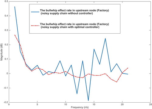
Figures 8 and 9 demonstrate the efficiency of the proposed method for the bullwhip effect reduction. As seen in Figure 8, the supply chain with controller has no bullwhip effect in the downstream nodes. Also, closed-loop systems can regulate the bullwhip in the upstream node.

Figure 8. The bullwhip effect in supply chain without controller and supply chain with controller.

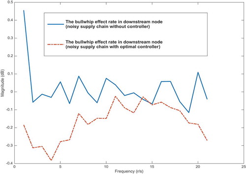
Figure 9. The bullwhip effect in supply chain without controller and supply chain with controller.

5. Simulation studies

We assume that the inventory obtained from the retailer, the recovery centre, the wholesaler and the factory have a normal white noise. This information has variance $Q_w$ while the measurement data have white noise with covariance $R_w$. The simulation was used to estimate the optimum data using non-linear optimal control for 100-day periods. The results reveal the optimal and accurate estimation for inventories for each level. In this supply chain, the retailer returns one-tenth of his inventory to the wholesaler for any reason and sends the same amount of inventory to the recovery centre for repairs. Also, the recovery centre immediately returns half of the stock to the factory.

Since the retailer node is a downstream member of the chain, its awareness of the customer real demand is due to self-prediction. Therefore, these nodes forecast their future order based on the customer previous demands. Note that the wholesaler orders are sent to the factory by taking into account its present inventory quantity.

In the second level of the supply chain, the wholesaler communicates with the retailer. The retailer orders are considered as the wholesaler inputs. Consequently, the wholesaler set its own next period demand based on the retailer previous orders. Also, in the third level of the supply chain, the manufacturer communicates with the wholesaler. Indeed, the wholesaler orders are considered as the input of this layer. Consequently, the manufacturer forecasts its next step inventory level based on the wholesaler previous orders.

In the following, non-linear quadratic Gaussian feedback control method will be utilized to restraint the bullwhip effect of the closed-loop supply chain with hybrid recycling channels and sale games. As mentioned above, the match production enterprise is called ‘Meshkin match’.

$x_1\left(k\right)$ is the factory inventory, I_1s represents the factory safety inventory, I_1e shows the factory expected inventory and I_1m denotes the factory maximum inventory. $x_2\left(k\right)$ is the wholesaler inventory, I_2s indicates the wholesaler safety inventory, I_2e reflects the wholesaler expected inventory and I_2m shows the wholesaler maximum inventory. $x_3\left(k\right)$ is the retailer inventory, I_3s represents the retailer safety inventory, I_3e is the retailer expected inventory and I_3m denotes the retailer maximum inventory. Table 2 reports real information, where $x_5\left(k\right)$ is the customer demand in step $t$. All of which have been normalized.

Table 2. Simulation data.

	Manufacturer	Wholesaler	Retailer
Initial inventory	200	170	100
Safety inventory	150	160	90
Expected inventory	400	180	120
Maximum inventory	600	200	130

$Q$ is the cost of inventory and $R$ represents the cost matrix of order. Figure 10 indicates the response of non-linear quadratic Gaussian optimal controller, compared with open-loop responses (the supply chain without controller).

Figure 10. Output of closed-loop supply chain (system with optimal controller).

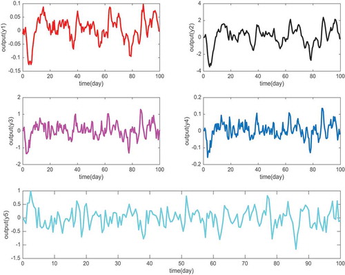
The response of open-loop supply chain to week disturbance (impulse) has been zero in the first 100 days. However, after step 90, the demand predicted by sales game approaches infinite.

As seen in Figure 10, with minimizing the cost of inventories and ordering, the designed supply chain with the controller can control fluctuations caused by the bullwhip effect in the chain. In the open-loop supply chain, the wholesaler inventory measured in 100 days tends to infinity and becomes unstable. Nevertheless, as mentioned for every node of the chain, we can keep the inventory level in a stable phase and minimize this stock cost.

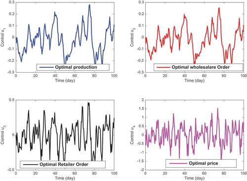
Given the cost of orders (control variables) and cost of inventories (state variables), to achieve an optimal index, control force is required. The retailer sends optimal orders to the wholesaler, after receiving demand of the downstream node (Figure 11(c)). The retailer adjusts the market demand in 20 days according to Figure 11. The wholesaler receives optimal order and adopts an optimal strategy to send for the factory in accordance with Figure 11(b). Ultimately, the factory will work to gain optimal inventory level based on Figure 11(a).

Figure 11. Optimal policy.

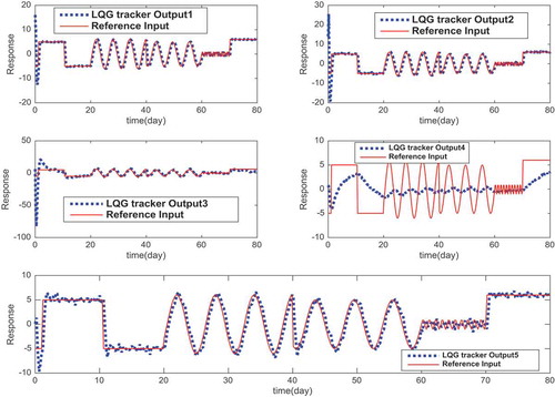
If the system becomes complicated by sending periodic requests to the retailer, then we have a tracker problem. The reference input (demand) provided by the customer in 80 days is shown in Figure 12. The closed-loop supply chain must minimize the cost and track reference input while also regulating the bullwhip effect.

Figure 12. LQG tracker.

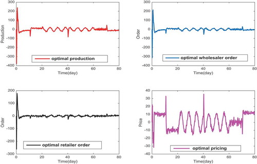
In order to track the demand from different markets, the manager must adopt a larger penalty for goods on days 2, 15, 40 and 75. The price strategy is displayed in Figure 13(d). The retailer must send optimal order according to Figure 13(c). This optimal strategy has oscillation during the first days, but after step 5, the domain of demand oscillation decreases gradually. The optimal order policy for the wholesaler is shown in part 2 in Figure 13. The last step of optimal control is the factory production (Figure 13(a)).

Figure 13. Optimal order, production and pricing.

Overall, managers can adapt the real supply chain model from the proposed one, sending optimal orders for the next periods (based on the LQG controller) by simulating and predicting market demands via the KF. Ultimately, such a strategy will adjust the inventory variances. The simulation results indicated the method efficiency.

6. Conclusion

In this paper, a model was developed for the hybrid recycling channel supply chain system. In this model, retailer attempts to achieve a large share of the competitive market with sales game and predicting market demand with consideration of demand as a decision-making variable. The forecasting method used by the retailer leads to uncertainty and unhealthy information. This issue results in complex and non-linear dynamic for supply chain. Also, stochastic noise in state variable and measurements leads to a stochastic system. We investigated the effect of these issues on the bullwhip effect and found that the mentioned factors lead to the bullwhip effect. In the non-linear supply chain, we proved that the bullwhip effect was happening. Without any lead time and gains, if the system has lead time, then the bullwhip effect has a direct relationship with this lead time. In the case of gain, the relation is not uniformly direct. Simulation and analytical results for stochastic noise effect on the bullwhip phenomenon showed that if we have the supply chain with stochastic noise, then the bullwhip effect occurs, where this relationship is uniformly direct. After probing the effects of noisy and complexity of the system, we investigated EKF method for reducing the stochastic noise in the system. Using EKF filter, we could provide an optimal estimate instead of ordinary demand forecasting method. Finally, non-linear quadratic Gaussian optimal controller could regulate the bullwhip effect. The results in the case study revealed that the proposed method for bullwhip was efficient.

So, to regulate the bullwhip effect, retailers who anticipate demands, should avoid the variable pricing as much as possible. All in all, price discounts in the online retail market amplify the bullwhip effect in the online retail supply chain [40]. Also, these price changes cause unpredictable phenomena such as the reverse bullwhip effect. Although demand forecasting methods complicate the system dynamics, they do not play a role in producing the bullwhip effect alone. Instead, the controller gain in the demand forecasting method and order time delay should be considered as appropriate to the model structure as possible. The wholesaler node receives a small share of the bullwhip effect. As a result, this node is a place where the manager can further adjust the fluctuations of the bullwhip effect. The stochastic noise contribution to the production of the bullwhip effect was higher than the other factors. Therefore, sharing information from the downstream to the upstream should be done with the least error (in line with the results of the Nagaraja et al.'s research [41]).

Non-linear quadratic Gaussian optimal controller can be easily extended to other multi-echelon supply chains with stochastic noise and complex dynamics. We suggest researchers to apply this method in power systems, economic systems, chemical engineering systems and so on. Also, due to the lack of comprehensive non-linear supply chain models, this non-linear model can be the starting point for controlling the bullwhip effect with other control methods. Time delays, demand forecasts, price discounts, stochastic noise, as well as periodic and stochastic demands are the main factors in creating the bullwhip effect. Note that control engineering has other powerful tools to control these factors. These methods can include fuzzy control, SMC, chaos control and a variety of other methods. For example, it is possible to control this phenomenon using SMC. Time delay is one of the main factors causing the bullwhip effect where non-linear control methods can be useful in the presence of delay. Given the powerful tools for analysing linear systems, a sublinear supply chain model from the proposed non-linear supply chain can be useful.

Disclosure statement

No potential conflict of interest was reported by the authors.

References

- B. Agaran, W.W. Buchanan, and M.K. Yurtseven, Regulating bullwhip effect in supply chain through modern control theory, IEEE Conference, USA, 2007.
- L. Beamon and M. Benita, Supply chain design and analysis: models and method, Int. J. Prod. Econ. 55 (1998), pp. 281–294. doi:10.1016/S0925-5273(98)00079-6.
- L. Pin-Ho, D. Shan-Hill, and J.S. Shang, Controller design and reduction of bullwhip for a model supply chain system using z-transform analysis, J. Process Control 14 (2004), pp. 487–499. doi:10.1016/j.jprocont.2003.09.005.
- J. Dejonckheere, S. Disney, M.R. Lambrecht, and D.R. Towill, Measuring and avoiding the bullwhip effect: a control theoretic approach, Eur. J. Oper. Res. 147 (2003), pp. 567–590. doi:10.1016/S0377-2217(02)00369-7.
- F.M. Asif, C.A. Bianchi, N. Rashid, and C.M. Niclescu, Performance analysis of the closed loop supply chain, J. Remanuf. 2 (1) (2012), pp. 1–21. doi:10.1186/2210-4690-2-4.
- N. Gao and S.M. Ryan, Robust design of a closed loop supply chain network for uncertain carbon regulations and random product flow, Euro. J. Transport. Logist. 3 (1) (2014), pp. 5–34. doi:10.1007/s13676-014-0043-7.
- F. Chen, Z. Drezner, J. Ryan, and D. Simchi-levi, Quantifying the bullwhip effect in a simple supply chain: the impact of forecasting, lead time, and information, Manage. sci. 46 (2000), pp. 436–443. doi:10.1287/mnsc.46.3.436.12069.
- J. Geunes, H.E. Romeijin, and K. Taaffe, Model for integrated production planning and order selection. Industrial Engineering Research Conference, IERC, Orlando, 2002.
- P.H. Zipkin, Foundations of Inventory Management, Mc Graw-Hill, New York, 2000.
- G.F. Franklin, J.D. Powell, and A. Emami, Feedback Control of Dynamic Systems, 4th ed., Prentice - Hall, New jersey, 2002.
- N.S. Nise, Control Systems Engineering, 3rd ed., John Wiley and Sons, Ins., New York, 2000.
- S. Benett, A brief history of automatic control, IEEE Control Syst. Mag. 16 (1996), pp. 17–25. doi:10.1109/37.506394.
- H.A. Simon, On the application of servomechanism theory in a study of production control, Econometrica 20 (1952), pp. 247–268. doi:10.2307/1907849.
- H.J. Vassian, Application of discrete variable servo theory to inventory control, Oper. Res. 3 (1955), pp. 272–282.
- U. Meyer and M.P. Groover, Multi echelon inventory systems using continuous systems analysis and simulation, AIIE Trans. 4 (1972), pp. 318–327. doi:10.1080/05695557208974869.
- J.F. Burns and B.D. Sivaslian, Dynamic analysis of multi-echelon supply systems, Comput. Ind. Eng. 2 (1978), pp. 181–193. doi:10.1016/0360-8352(78)90010-4.
- S. John, M.M. Naim, and D.R. Towill, Dynamic analysis of a WIP compensated decision support system, Int. J. Manuf. Syst. Des 1 (1994), pp. 283–297.
- J. Dejonckheere, S.M. Disney, M.R. Lambrecht, and D.R. Towill, The impact of information enrichment on a bullwhip effect in supply chain: a control engineering perspective, Eur. J. Oper. Res. 153 (2004), pp. 727–750. doi:10.1016/S0377-2217(02)00808-1.
- S.M. Disney and D.R. Towill, On the bullwhip and the inventory variance produced by an ordering policy, Omega 31 (2003), pp. 157–167. doi:10.1016/S0305-0483(03)00028-8.
- P. Ignaciuk and A. Bartoszewicz, Linear - quadratic optimal control of periodic-review perishable inventory systems, IEEE Trans. Control Syst. Technol. 20 (5) (2012). doi:10.1109/TCST.2011.2161086
- S. Chandra, S.,.M. Lalwani, D.R. Disney, and L. Towill, Controllable, observable and stable state space representation of generalized order-up-to policy, Int. J. Prod. Econ. 101 (2006), pp. 172–184. doi:10.1016/j.ijpe.2005.05.014.
- F. Dongfei, I. Clara, A. El-Houssaine, and K. Robin, Quantifying and mitigating the bullwhip effect in a benchmark supply chain system by an extended prediction self-adaptive control ordering policy, Comput. Ind. Eng. 81 (2015), pp. 46–57. doi:10.1016/j.cie.2014.12.024.
- W.C. Li, Y. Jing, W. Wang, and L. Deng, Dynamic model and robust H infinity control of remanufacturing system whit hybrid recycling channels, Syst. Eng. 30 (2012), pp. 51–56.
- Y.Y. Yi and J.M. Liang, Hybrid recycling modes for closed loop supply chain under premium and penalty mechanism, Comput. Int. Manuf. Sys. 20 (2014), pp. 215–223.
- X.P. Hang, Z.J. Wang, and H.G. Zhang, Decision models of closed loop supply chain with remanufacturing under hybrid dual-channel collection, Int. J. Adv. Manuf. Techol. 68 (5–8) (2013), pp. 1851–1865. doi:10.1007/s00170-013-4982-1.
- S.T. Zhang and X.W. Zhao, Fuzzy robust control for an uncertain switched dual-channel closed loop supply chain model, IEEE Trans. Fuzzy Sys. 23 (2015), pp. 485–500. doi:10.1109/TFUZZ.2014.2315659.
- Z.H. Xiu and G. Ren, Stability analysis and systematic design of T-S fuzzy control system, Fuzzy Sets Syst. 151 (2005), pp. 119–138. doi:10.1016/j.fss.2004.04.008.
- S. Zhang, X. Li, and C. Zhang, A fuzzy control model for restrain of bullwhip effect in uncertain closed loop supply chain whit hybrid recycling channels, Trans. Fuzzy Syst. 25 (2016), pp. 457–482.
- M. Goodarzi and R. Farzipoor, How to measure bullwhip effect by network data envelopment analysis? J. Comput. Ind. Eng. (2018). doi:10.1016/j.cie.2018.09.046.
- K. Govindan, M. Fattahi, and E. Keyvanshokooh, Supply chain network design under uncertainty: a comprehensive review and future research directions, J. Eur. J. Oper. Res. (2017). doi:10.1016/j.ejor.2017.04.009.
- P. Ignaciuk and A. Bartoszewicz, LQ optimal sliding mode supply policy for periodic review inventory systems, IEEE Trans. Autom. Control 55 (1) (2010), pp. 269–274. doi:10.1109/TAC.2009.2036305.
- P. LeVniewski and A. Bartoszewicz, LQ optimal sliding mode control of periodic review perishable inventories with transportation losses, Math. Prob. Eng. (2013), pp. 1–9. Article ID 325274. doi:10.1155/2013/325274.
- A. Bartoszewicz and P. Latosi´nski, Sliding mode control of inventory management systems with bounded batch size, J. Appl. Math. Model. (2018). doi:10.1016/j.apm.2018.09.010.
- L. Wandong, M. Junhai, and Z. Xueli, Bullwhip entropy analysis and chaos control in the supply chain with sales game and consumer returns, Entropy 64 (2017), pp. 1–19.
- S. Torabi, A. Morteza, and M. Moghadam, Provide a new approach to decision-making on demand management and production planning, Ind. Eng. J. Iran 45 (2011), pp. 31–44.
- T. Li and J. Ma, Complexity analysis of the dual-channel supply chain model with delay decision, Nonlinear Dyn. 78 (2014), pp. 2617–2626. doi:10.1007/s11071-014-1613-9.
- X. Wang and S.M. Disney, Mitigating variance amplification under stochastic lead-time: the proportional control approach, Eur. J. Oper. Res. 256 (1) (2017), pp. 151–162. doi:10.1016/j.ejor.2016.06.010.
- J. Hartikainen, A. Solin, and S. Särkka, Optimal Filtering with Kalman Filters and Smoothers, Department of Biomedical Engineering and Computational Science, Aalto University School of Science, Finland, 2011.
- D.E. Krik, Optimal Control Theory, Prentice-Hall, Englewood Cliffs New Jersey, 1990.
- D. Gao, N. Wang, Z. He, and T. Jia, The bullwhip effect in an online retail supply chain: a perspective of price-sensitive demand based on the price discount in ecommerce, IEEE Trans. Eng. Manage. 64 (2) (2017), pp. 134–148. doi:10.1109/TEM.2017.2666265.
- C.H. Nagaraja and T. McElroy, The multivariate bullwhip effect, Eur. J. Oper. Res. 267 (1) (2018), pp. 96–106. doi:10.1016/j.ejor.2017.11.015.