Quantum-computing with AI & blockchain: modelling, fault tolerance and capacity scheduling

ABSTRACT

We model the hardware and software architecture for generalized Internet of Things (IoT) by quantum cloud-computing and blockchain. To reduce the measurement error and increase the efficiency of quantum entanglement (i.e. the capability of fault tolerance) in the current quantum computers and communications, we design a quantum-computing chip by modelling it as a multi-input multi-output (MIMO) quantum channel and obtain its channel capacity via our recently derived mutual information formula. To capture the internal qubit data flow dynamics of the channel, we model it via a deep convolutional neural network (DCNN) with generalized stochastic pooling in terms of resource-competition among different quantum eigenmodes or users. The pooling is corresponding to a resource allocation policy with two levels of competitions as in cognitive radio: the first one is on users’ selection in a ‘win–lose’ manner; the second one is on resourcesharing among selected users in a ‘win–win’ manner. To wit, our scheduling policy is the one by mixing a saddle point to a zero-sum game problem and a Pareto optimal Nash equilibrium point to a nonzero- sum game problem. The effectiveness of our policy is proved by diffusion modelling with theory and numerical examples.

KEYWORDS:

• Quantum-computing modelling
• blockchain
• IoT and DCNN

1. Introduction

With the emergence of quantum-computing (see, e.g. Courtland [1], Dai [2], Deutsch [3], Feynman [4], Gibney [5], Nielsen and Chuang [6]), the currently implementing Industrial 4.0 (IR 4.0, see, e.g. Schwab [7]) will be quickly evolving to Industrial 6.0 (IR 6.0, see, e.g. SIR (Sixth Industrial Revolution) Forum [8]). SIR Forum is an U.S. Los Angeles based Forum and was founded in February of 2018. It foresaw that the quantum computing and blockchain will be the core technology of IR 6.0. Comparing with the today’s system, the future quantum system will have extremely powerful processing, storage, tracing and management capability with strong artificial intelligence (AI), which makes the future (strong or generalized) Internet of Things (IoT) possible. This generalized IoT can be called as Internet of Every Thing (see, e.g. Figure 1; Dai [2] and Santucci [9]).

Figure 1. Evolution of industrial revolution and internet of every thing (IoT).

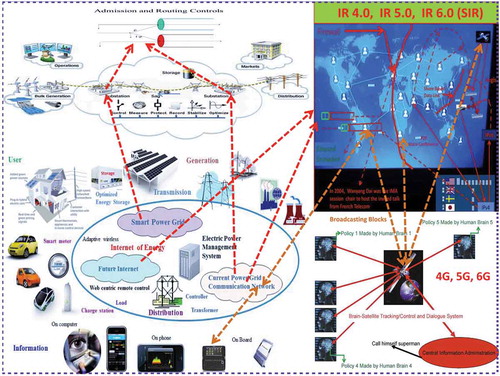
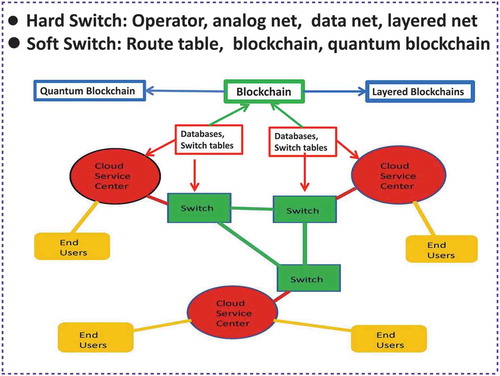
Conceptually, an IoT consists of two parts: Internet and Things. However, the most important feature in an IoT is the efficient interaction between Internet and Things. To reach the efficiency, it requires high-performance network hardware and intelligent softwares with effective integration to realize the future Internet as designed in Figure 1. More precisely, inside the IoT network system, there is an interactive hardware and software system as structured in Figure 2. To realize the interaction between Internet and Things, hardware quantum computing centres and physical Things must be integrated together as in Figure 4 through a data storage and software managing system called quantum blockchain as in Figure 4 with flow chart in Figure 3. Note that, in Figure 4, we consider the Thing as the future quantum MIMO wireless channel, which reflects the trend of future advancements on mobile cloud-computing (see, e.g. Dai [10]).

Figure 2. Blockchain protocol evolution and quantum network architecture.

In the current era of Industrial 4.0, Things in an IoT (see. e.g. the left-hand side in Figure 1) represent the real-world application systems that can be the intelligent end-user’s devices or their generalized forms such as a power and energy system or a supply chain system (see, e.g. Artemis [11] and Dai [2]). However, in the defined Industrial 5.0 of human–machine interactions, Things in an IoT can even be our own human beings (see, e.g. the lower-right graph in Figure 1; Dai [12] and Haykin [13]). The interactions between Internet and Things in an IoT can be realized through optical fibre linkages or wireless multi-input multi-output (MIMO) communication (e.g. 4G, 5G or even the future 6G) channels as shown in Figure 1 and as discussed in Dai [2]. In an IoT, Internet is the major information processing and transmission system (see, e.g. its network architecture in Figure 2 and the study in Dai [14]).

It was originated from the U.S. based ARRP (Advanced Research Projects Agency) and initially implemented in U.S. Navy around the late 1960s (see, e.g. Comer [15]) and then went to civil usage. Traditionally, the transmitted IP packet in each node is not stored or not fully stored due to the limitation of processing and storage capacity. Nevertheless, with the increasing of the service capacity, the blockchain technology with data storage at each node becomes implementable and is even predicted its usage in the U.S. Navy Aegis communication system with the encryption of 256 bit Hashes (see, e.g. Figure 1). Furthermore, to further its efficiency and security, quantum computers come up such as IBM 50-qubit, Google 72-qubit and Rigetti 128-qubit quantum computers. With the enhancements of these quantum computers, the new quantum-computing Moore’s law (see, e.g. Bertels [16]) targeting the realization of a $n$-qubit based quantum computing for a continuously increasing number $n$ is emerging. When $n$ is larger, the corresponding computation power will meet the needs of many real-world applications, e.g. 30-qubit = 10 trillion floating-point operation and 50-qubit = 10 billions of billion floating-point operation (see, e.g. Fan [17]). Thus, we can predict that the current internet protocol (IP) and MIMO communication network will be replaced by quantum IP and quantum MIMO based ones around the next 25 years. Moreover, they will be powered by quantum-cloud-computing and quantum blockchain with the storage capability in each service centre and switch node (see, e.g. Figure 2 and Dai [14]). From one end-user to another one, the user’s quantum data flow consists of qubit data packets will be transmitted from one quantum cloud-computing centre to another one via quantum IP managed by network quantum blockchain software management system (see, e.g. the quantum IP network in Figure 1 with embedded blockchain in Figure 3, and the discussions in Dai [2], Rajan and Visser [18]). For future references, we call this quantum IP network as a QBP internet (a quantum-blockchain-protocol based internet).

Figure 3. Quantum-blockchain evolution and processing chart.

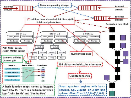
Blockchain is a quickly developing data storage and service technology, which is widely used in IoT, FinTech, Bitcoin/Ethereum, and other applications (see, e.g. Dai [2], Buterin [19], Iansiti and Lakehani [20], Nakamoto [21]) with the functionalities of blockchain management, transaction generation, node communication and block mining. More precisely, blockchain is an orderly distributed database (or called a ledger) system with processing chart of software architecture as presented in Figure 3. With the appearance of real quantum computers built from IBM, Google, Rigetti, D-Wave, etc., it is recently evolving to the quantum-blockchain by substituting the standard cryptographic Hash functions to quantum cryptographic Hash functions (see, e.g. Rajan and Visser [18]). Unchangeable data history and highly secured signature procedure make each trading transaction more safe than ever. Smart contracts in conducting block mining and flexible node communications make it realizable for the blockchain management to be decentralized and can be realized by implementing strategies through running various algorithms aided with AI. In doing so, the efficient interaction between blockchain and its supporting high-performance quantum-computing hardware facilities is a necessity (see, e.g. Figure 4 and Dai [2]).

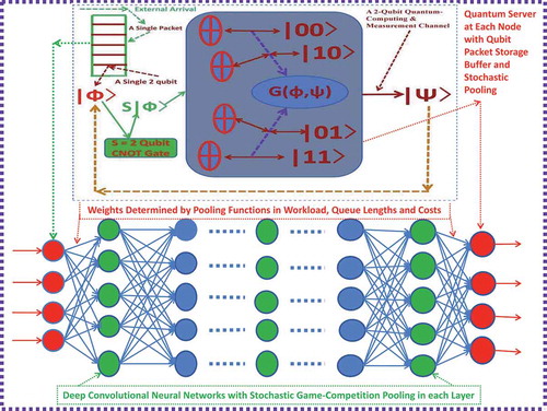
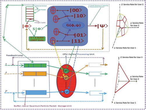
Figure 4. A quantum computing platform with parallel-queues and multiple pools. The upper-left blockchain is from Dai [2] and is detailed in Figure 3. The lower-right graph is a quantum MIMO wireless channel.

Currently, there are numerous physical realizations of quantum computers (e.g. those announced by IBM, Google, Rigetti and D-Wave), which are mainly based on four quantum computing models of practical importance besides the theoretical quantum Turing machine (see, e.g. see, e.g. Deutsch [3], Feynman [4], Nielsen and Chuang [6]). However, the performance of these quantum computers still has much more room to improve in terms of error measurement, computing efficiency, energy consumption and cost. Hence, in this paper, we first propose a quantum-computer chip by modelling it as an MIMO channel. This design was originally announced by Dai [22] as a keynote speech in an IEEE conference. Here, we further formalize it and try to make it publicly available. Then, by the mutual information formula derived in Dai [23], we can study the quantum entanglement and fault tolerance concerning signal measurements and determine the service capacity for our proposed quantum channels. During the procedure, there are two types of problems involved: how to allocate power (or rate) resource to different eigenmodes in a quantum-computing channel and how to allocate the rate resource to different users in quantum-cloud-computing service centres. To solve these problems, we model the internal qubit data flow dynamics of the quantum channel through a deep convolution neural network (DCNN) with generalized stochastic pooling in terms of resource-competition users (see, e.g. Figure 5).

Figure 5. An DCNN with quantum processor and generalized stochastic pooling. The upper graph is adapted from Figure 8.

This dynamical system is corresponding to a so-called game platform that was initially studied in Dai [2,24]. To be consistent with the study in the current AI era, we here use the terminology ‘DCNN with stochastic pooling’ (see, e.g. Zeiler and Fergus [25]) to replace the original one to describe the data flow dynamics in our ‘game platform’. Furthermore, in the studies of Dai [2,24], only a ‘win–win’ non-zero-sum Pareto optimal Nash equilibrium policy was designed dynamically. However, in this paper, we extend this policy to allow the stochastic pooling in our DCNN to have one more competition level with ‘win–lose’ users. In other words, our generalized policy is the one by mixing a saddle point to a zero-sum game problem and a Pareto optimal Nash equilibrium point to a non-zero-sum game problem, which can also be used in more other applications, such as, cognitive radio (see, e.g. Akyildiz et al. [26], Haykin [13]), Internet of Energy (IoE, see, e.g. Artemis [11] and Dai [2]) and FinTech (see, e.g. Buterin [19], Nakamoto [21]).

More precisely, in our game platform, we use the triply stochastic renewal reward process (TSRRP) studied in Dai [2] to model the random dynamics of the input quantum qubit data packet flows (or called big data flows, see, e.g. De Mauro et al. [27], Dedić and Stanier [28], Snijders et al. [29]). Furthermore, as in Dai [2], we model the dynamical rate capacity available for resource-competing users at each channel or service pool as a randomly evolving capacity region driven by a finite state continuous Markov chain (FS-CTMC). The parallel-queues in this platform (see, e.g. Figures 3 and 4) are used to storage and buffer quantum qubit data packets from their corresponding users. Each queue may be served simultaneously by multiple intelligent quantum-computing channels or service pools while each channel or pool may also serve multiple queues at the same time via running smart policies in the blockchain (see, e.g. Figure 4). However, to reflect the dynamic evolving nature of real-world systems and to realize the decentralized operation in a blockchain, the users to be selected at a time is random, the number of pools to serve a particular queue is random, and the number of queues to be served by a particular pool is also random. The efficiency or optimization concerning our designed policy is in terms of system delay, revenue, profit, cost, etc. We will model them through certain utility functions with respect to the performance measures of their internal quantum qubit data flow dynamics such as queue length and workload processes. To illustrate the effectiveness of our policy, we establish a reflecting diffusion with regime-switching (RDRS) model for the performance measures under our proposed policy in order to offer services to different users in an optimal and fair way. Based on this RDRS model, our designed policy is effectively implemented with numerical examples.

The remainder of the paper is organized as follows. In Section 2, we present the quantum system formulation modelled by MIMO channels, fault tolerance by quantum mutual information, quantum storage and particle queueing dynamics. In Section 3, we present the RDRS model and the performance modelling for its internal quantum qubit data flow dynamics of the modelled quantum channel by the RDRS model. Main DCNN and game-competition based scheduling policy together with theoretical modelling results are presented. Numerical simulation examples are also given in this section. In Section 4, we formally prove our main theoretical results. In Section 5, we conclude the paper with remarks.

2. Quantum system formulation modelled by MIMO channels

This section consists of two subsections: qubit presentation and quantum mutual information, quantum storage and particle queueing dynamics.

2.1. Qubit presentation and quantum mutual information

In a quantum-computing-based computer or communication system, the basic information unit is a $n$-qubit with $n\in \{1,2,...\}$ and can be expressed through the conventional complex column-vector oriented ket-notation. More precisely, a state $|\mathrm{\Psi }⟩$ of $n$-qubit register is represented by

(2.1) $|\mathrm{\Psi }⟩=\sum _{j_l\in \{0,1\},l\in \{1,...,n\}}{\psi }_{j_1...j_n}|j_1...j_n⟩,$(2.1)

where, $|j_1...j_n⟩$ for each $j_l\in \{0,1\}$ and $l\in \{1,...,n\}\}$ is called an eigenstate and there are total number $2^n$ of them. In the meanwhile, the basis of bit strings $\{j_1...j_n:j_l\in \{0,1\},l\in \{1,...,n\}\}$ is known as the computational basis with the corresponding complex coefficients denoted by $\{{\psi }_{j_1...j_n}\}$. For example, a special case corresponding to the expression in (2.1) with $n=1$ and ${\psi }_0={\psi }_1=1/\sqrt{2}$ can be realized via the Hadamard gate $H$ (see, e.g. Deutsch [3], Feynman [4], Nielsen and Chuang [6]) as follows,

$H=\frac{1}{\sqrt{2}}\left(\begin{array}{cc}1& 1\\ 1& -1\end{array}\right),$

$H|0⟩=(|0⟩+|1⟩)/\sqrt{2},$

$H|1⟩=(|0⟩-|1⟩)/\sqrt{2}.$

The sum of the squares of the coefficients’ absolute values in (2.1) must be the unity, i.e.

(2.2) $\sum _{j_l\in \{0,1\},l\in \{1,...,n\}}{\left|{\psi }_{j_1...j_n}\right|}^2=1.$(2.2)

For each bit string, $j_1...j_n$, $|{\psi }_{j_1...j_n}{|}^2$ gives the probability of the system being found in the $(j_1...j_n{)}^{th}$ state after a measurement. However, because a complex number encodes not just a magnitude but also a direction in the complex plane, the phase difference between any two coefficients (states) denotes a meaningful parameter. This is a fundamental difference between quantum computing and probabilistic classical computing. Under this computational basis, a state $|\mathrm{\Psi }⟩$ of $n$-qubit register can be represented by its coefficients $\{{\psi }_{j_1...j_n}\}$. For examples, if $n=3$, $|010⟩=(0,0,1,0,0,$ $0,0,0)\prime$ and if $n=1$, $|0⟩=(1,0)\prime$ while $|1⟩=(0,1)\prime$, where, the prime denotes the transpose of a vector. 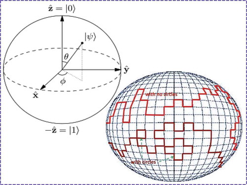Note that, if $n=1$, a single qubit can be used to denote a particle spinning up and down at the same time. The possible quantum states for a single qubit is visualized by the so-called Bloch sphere as in the left-upper graph of Figure 6, where $|\mathrm{\Psi }⟩={\psi }_0|0⟩+{\psi }_1|1⟩\mathrm{w}\mathrm{i}\mathrm{t}\mathrm{h}{\psi }_0=cos\left(\theta /2\right)\mathrm{a}\mathrm{n}\mathrm{d}\beta =e^{i\varphi }sin(\theta /2)$. Note that, the Bloch sphere is the surface of a ball and hence is a two-dimensional manifold since it can be represented by a collection of two-dimensional maps. In the sequel, we just simply call it a 2-sphere by mathematical convention. A pure qubit state can be represented by any point on such a 2-sphere with corresponding angles $\theta$ and $\varphi$. More precisely, $\theta$ is the angle between $z$-axis and $|\mathrm{\Psi }⟩$, and $\varphi$ is the angle between $x$-axis and the projection of $|\mathrm{\Psi }⟩$ onto $xy$-plane.

Figure 6. Qubit representation and random walk.

In the future quantum cloud-computing and communication system (see, Figure 2 for a newly designed example), the traditional binary (zero or one) bit based data packets will be replaced by quantum data packets. Each of them will consist of user’s data payload and packet head that indicates the service requirements managed by system software called quantum blockchain in Dai [2] (see, Figure 4 for detail). The length of a quantum data packet is the number of qubits randomly walking over the Bloch sphere as shown in the lower-right graph of Figure 6. Note that, the random step size for each walk along a particular direction over the sphere may be greater than the unity. Furthermore, the packet length is also random from one quantum data packet to another one. However, no matter whether in a quantum computer or in a quantum communication channel, the service time and quality for a quantum data packet depends on the measurement of each single source qubit. Currently, there are numerous physical realizations of quantum computers, which are mainly based on four quantum computing models of practical importance besides the theoretical quantum Turing machine (see, e.g. Deutsch [3], Feynma [4], Nielsen and Chuang [6]). However, the error from the measurement or unitary operation is still the issue. In general, due to the non-cloning theorem (see, e.g. Niestegge [30], Wootters and Zurek [31]), unknown pure quantum states cannot be copied unless they are orthogonal. Nevertheless, according to Niestegge [30] and references therein, the approximate or imperfect cloning of quantum states is possible, e.g. via a generalized non-Gaussian mutual information formula (see, e.g. Dai [23]) by developing a quantum channel between quantum states and their measurements (or their received states) in a probabilistic way. Furthermore, the quantum Zeno effect or called Zeno’s paradox (i.e. the inhibition of transitions between quantum states by frequent measurements, see, e.g. Itano et al. [32], Misra and Sudarshan [33]) is the other concerned issue. Nevertheless, inside the recently realized IBM 50 qubit quantum computer, the quantum coherence time (the time gap to keep a channel stable (i.e. to keep the number of quantum states the same)) can last up to 90 μs to reduce the influence of Zeno effect, which is enough for the quantum computer to perform the required operation and realize one 20-qubit quantum entanglement in 187 ns (see, e.g. the latest announcement in Song et al. [34]). Therefore, with the hope to reduce the error, we develop a quantum channel method in performing the measurement and computation, which is evolved from the one currently being implemented in MIMO wireless channel (see e.g. Dai [2,24]). An example of such a quantum channel is presented in the lower graph of Figure 7 and illustrated via a comparison with an MIMO channel in the upper-left graph of the figure.

More precisely, consider a quantum state $|\mathrm{\Psi }⟩$ as a wave-packet and suppose that there is an eigenmode corresponding to each eigenstate $|j_1...j_n⟩$ with $j_l\in \{0,1\}$ and $l\in \{1,...,n\}$ in the $n$-qubit register of (2.1). The processing based on a single $n$-qubit chip (e.g. the one designed in the lower graph of Figure 7) is more like the one in a single-user MIMO wireless broadcast channel (currently used for 4G/5G wireless communications, see, e.g. Dai [2,24]).

Figure 7. A comparison between $1$-qubit quantum chip in the lower graph and OAM MIMO channel in the upper-left graph, which is illustrated via an intermediate double-slit experiment in the upper-right graph. Channel function $G(\mathrm{\Phi },\mathrm{\Psi })$ is derived in (2.10). The two upper graphs are not parts of our designed quantum channel, which are presented only for the purpose of comparison and illustration.

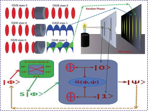
In the upper-left graph of Figure 7, an orbital angular momentum (OAM) channel (i.e. a particular MIMO channel) is pictured, where, each output wave is with given deterministic frequency and phase. However, to be more illustrative, let us observe the upper-right graph (enhanced from Chang [35]) of Figure 7 for a double-slit experiment, bifurcation occurs along the moving paths of quantum particles (see, e.g. Dai [23]). In other words, the output wave is uncertain due to the random phases associated with different quantum particles, which is also related to quantum walks with random phase shifts (see, e.g. Košík et al. [36]). Therefore, the input/output waves in this quantum-computing system form a probabilistic MIMO channel (see, e.g. in the lower graph of Figure 7) and it can be modelled in a generalized way as follows.

Each eigenmode is with power allocation $P_{|j_1...j_n⟩}$ and the total power allocation on the chip processing is subject to a constraint $P$ such that

(2.3) $\sum _{j_l\in \{0,1\},l\{1,...,n\}}{P}_{|j_1...j_n⟩}=P.$(2.3)

A $n$-qubit may be measured in a quantum computer or a quantum communication network. In the later case, some switch functionality may also be involved (e.g. for an entanglement between two qubits and see Sawerwain and Wiśniewska [37] for a reference). Thus, we add a switch gate $S$ to our quantum channel. For a quantum state $|\mathrm{\Phi }⟩$ with complex coefficients $\{{\varphi }_{j_1...j_n},j_l\in \{0,1\},l\in \{1,...,n\}\}$, its corresponding state after switching is denoted by $S|\mathrm{\Phi }⟩$. If the quantum gate $S$ takes an identity matrix $I$, this gate placed in a quantum circuit does not perform any operation on the $n$-qubit, e.g. $S|\mathrm{\Phi }⟩=I|\mathrm{\Phi }⟩=|\mathrm{\Phi }⟩$. However, in a general situation, the gate $S$ will do the required switch operations. For examples, we can take $S$ to be a $1$-qubit Pauli gate $X$ or a $2$-qubit $CNOT$ gate to perform the switch functionality,

(2.4) $X=\left(\begin{array}{cc}0& 1\\ 1& 0\end{array}\right),CNOT=\left(\begin{array}{cccc}1& 0& 0& 0\\ 0& 1& 0& 0\\ 0& 0& 0& 1\\ 0& 0& 1& 0\end{array}\right).$(2.4)

Then, we have the following switch results corresponding to $n=1$ and $n=2$, respectively,

$\begin{array}{rl}& CNOT|00⟩=|00⟩,\\ & X|0⟩=|1⟩,CNOT|01⟩=|01⟩,\\ & X|1⟩=|0⟩,CNOT|10⟩=|11⟩,\\ & CNOT|11⟩=|10⟩.\end{array}$

Furthermore, let $\mathcal{H}(\varphi )$ be the column vector formed by $\{{\varphi }_{j_1...j_n}\}$ and ${\mathcal{H}}^{†}(\varphi )$ be its associated row vector formed by the conjugate complex numbers $\{{\varphi }_{j_1...j_n}^{†}\}$. To be more illustrative, we use an index $h\in \{h_0,h_1,...,h_{2^n-1}\}=\{0,1,...,2^n-1\}$ to denote its corresponding index $j_1\cdot \cdot \cdot j_n$ in (2.1) for an integer $j_l\in \{0,1\}$ and each number $l\in \{1,...,n\}$ as follows,

(2.5) $h=2^{n-1}{j}_n+2^{n-2}{j}_{n-1}+...+2j_2+j_1.$(2.5)

Then, $\mathcal{H}(\varphi )$ and ${\mathcal{H}}^{†}(\varphi )$ can be explicitly expressed by

(2.6) $\mathcal{H}(\varphi )=({\varphi }_{h_0},...,{\varphi }_{h_{2^n-1}})\prime ,{\mathcal{H}}^{†}(\varphi )=({\varphi }_{h_0}^{†},...,{\varphi }_{h_{2^n-1}}^{†}).$(2.6)

Furthermore, let $e(n)$ be the $2^n\times 2^n$ matrix given by

(2.7) $e(n)=(|h_0⟩|h_1⟩\cdot \cdot \cdot |h_{2^n-1}⟩),$(2.7)

where, $|h_i⟩$ with an $i\in \{0,1,...,2^n-1\}$ is a column vector corresponding to a $|j_1\cdot \cdot \cdot j_n⟩$ for an integer $j_l\in \{0,1\}$ and each number $l\in \{1,...,n\}$. Thus, $n$-qubits $S|\mathrm{\Phi }⟩$ and $|\mathrm{\Psi }⟩$ can be denoted by

(2.8) $S|\mathrm{\Phi }⟩=Se(n)\mathcal{H}(\varphi ),|\mathrm{\Psi }⟩=e(n)\mathcal{H}(\psi ).$(2.8)

Thus, under the assumption that the matrix $\mathcal{H}(\varphi ){\mathcal{H}}^{†}(\varphi )$ is invertible, we can conclude that

(2.9) $e(n)=|\mathrm{\Phi }⟩{\mathcal{H}}^{†}(\varphi ){\left(\mathcal{H}(\varphi ){\mathcal{H}}^{†}(\varphi )\right)}^{-1}.$(2.9)

Furthermore, by the expressions in (2.1), (2.8) and (2.9), we can derive a quantum-computing and measurement channel (i.e. a quantum communication channel with an example in Figure 8) between the original $n$-qubit $|\mathrm{\Phi }⟩$ and the measured $n$-qubit $|\mathrm{\Psi }⟩$ as follows,

(2.10) $|\mathrm{\Psi }⟩=|\mathrm{\Phi }⟩{\mathcal{H}}^{†}(\varphi ){\left(\mathcal{H}(\varphi ){\mathcal{H}}^{†}(\varphi )\right)}^{-1}\mathcal{H}(\psi ).$(2.10)

Figure 8. A 2-qubit quantum-computing and measurement channel with channel function $G(\mathrm{\Phi },\mathrm{\Psi })$ derived in (2.10).

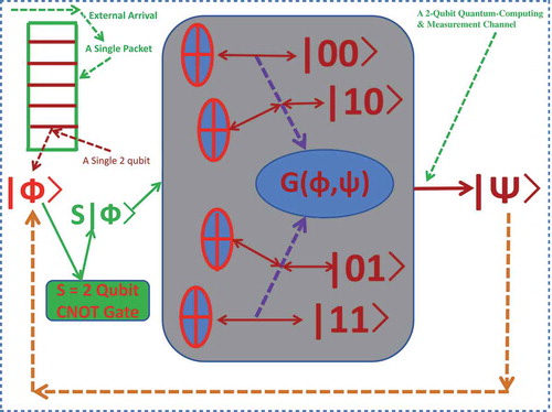
Thus, we are aimed to measure $|\mathrm{\Phi }⟩$ through $|\mathrm{\Psi }⟩$ in (2.10) as accurate as possible. The ideal case is such that the measurement has the closest quantum entanglement properties between $S|\mathrm{\Phi }⟩$ and $|\mathrm{\Psi }⟩$ in terms of position, momentum, spin and polarization (see, e.g. Deutsch [3], Feynman [4], Nielsen and Chuang [6]). Since $S|\mathrm{\Phi }⟩$ in (2.10) is random with distribution $S(|{\varphi }_{\mathrm{0...0}}{|}^2,...,|{\varphi }_{j_1...j_n}{|}^2,...,|{\varphi }_{\mathrm{1...1}}{|}^2)\prime$, we use $M$ to denote its covariance matrix and let $\mathrm{T}\mathrm{r}(M)$ be its trace. If we endow each eigenmode with the power $P_{j_1...j_n}$, i.e. $(\mathrm{T}\mathrm{r}(M){)}_{j_1...j_n}\le P_{j_1...j_n}$, an MIMO MAC channel will be related (see, e.g. Dai [24] and Goldsmith et al. [38]). However, if we endow the whole quantum computer chip with the total power $P$, i.e. $\mathrm{T}\mathrm{r}(M)\le P$, an MIMO BC channel will be concerned (see, e.g. Dai [24] and Goldsmith et al. [38]). In both cases, the maximal transmission rates or minimal error measurements can be reached by applying mutual information formulas and water-filling coding techniques (see, e.g. Cover and Thomas [39], Dai [23], Goldsmith et al. [38]).

2.2. Quantum storage and particle queueing dynamics

In this subsection, we assume that the quantum cloud-computing and communication system has $V$ service pools (indexed by a set of positive integers $\mathcal{V}\equiv \{1,...,V\}$) and $J$ queues in parallel (indexed by $j\in \mathcal{J}\equiv \{1,...,J\}$ and corresponding to $J$ users) as shown in Figure 4. Each pool is equipped with $J_v$ number of flexible quantum-computer based parallel-servers, where $v$ is an integer in $\mathcal{V}$. Associated with the queues, there is an $J$-dimensional quantum data packet arrival process $A=\{A(t)=(A_1(t),...,A_J(t))\prime ,$ $t\ge 0\}$, where $A_j(t)$ with $j\in \mathcal{J}$ and $t\ge 0$ is the number of $n$-qubit data packets that arrive at the $j$th queue during $(0,t]$. Note that, here and elsewhere in the paper, the prime denotes the transpose of a vector or a matrix. The size of the quantum data packet is supposed to be a random number $\zeta \in \{1,2,...\}$. In other words, each quantum data packet can be denoted by a sequence of $n$-qubits $\{|{\mathrm{\Phi }}_1⟩,...,|{\mathrm{\Phi }}_{\zeta }⟩\}$, where, $|{\mathrm{\Phi }}_i⟩$ for each $i\in \{1,2,...,\zeta \}$ denotes a $n$-qubit. For example, the single packet shown in the upper-left corner of Figure 8 consists of seven $2$-qubits including the two green ones, i.e. $\zeta =7$. The whole system is supposed to be driven by a stationary FS-CTMC $\alpha =\{\alpha (t),t\in [0,\mathrm{\infty })\}$ with a finite state space $\mathcal{K}\equiv \{1,...,K\}$. The generator matrix of $\alpha (\cdot )$ is denoted by $G=(g_{il})$ with $i,l\in \mathcal{K}$, and

(2.11) $g_{il}=\left\{\begin{array}{cc}-\gamma (i)& \mathrm{i}\mathrm{f}i=l,\\ \gamma (i)q_{il}& \mathrm{i}\mathrm{f}i\ne l,\end{array}\right.$(2.11)

where, $\gamma (i)$ is the holding rate for the chain staying in a state $i\in \mathcal{K}$ and $Q=(q_{il})$ is the transition matrix of its embedded discrete-time Markov chain (see, e.g. Resnick [40]). Furthermore, let ${\tau }_n$ for each nonnegative integer $n\in \{0,1,...\}$ be defined by

(2.12) ${\tau }_0\equiv 0,{\tau }_n\equiv inf\{t>{\tau }_{n-1}:\alpha (t)\ne \alpha (t^{-})\}.$(2.12)

In other words, ${\tau }_n$ is a random jump time of the Markovian process $\alpha (\cdot )$. As in Dai [2], we model the arrival process $A_j(\cdot )$ for each $j\in \mathcal{J}$ by an TSRRP, and for convenience, we recall the definition of an TSRRP as follows.

Definition 2.1 A process $A_j(\cdot )$ with $j\in \mathcal{J}\equiv \{1,...,J\}$ is called an TSRRP if $A_j({\tau }_n+\cdot )$ for each $n\in \{0,1,...\}$ is the counting process corresponding to a (conditional) delayed renewal reward process with arrival rate ${\lambda }_j(\alpha ({\tau }_n))$ and mean reward $m_j(\alpha ({\tau }_n))$ associated with finite squared coefficients of variations ${\alpha }_j^2(\alpha ({\tau }_n))$ and ${\zeta }_j^2(\alpha ({\tau }_n))$ during time interval $[{\tau }_n,{\tau }_{n+1})$.

In addition, we let $\{u_j(k),k=1,2,...\}$ be the sequence of times between the arrivals of the $(k-1)$th and the $k$th reward batches of packets at the $j$th queue. The corresponding batch reward is denoted by $w_j(k)$ and all the packets arrived with it are indexed in certain successive order. Then, we can define the renewal counting process associated with the inter-arrival time sequence $\{u_j(k),k=1,2,...\}$ for each $j\in \mathcal{J}$ by

(2.13) $N_j(t)=sup\left\{n\ge 0:\sum _{k=1}^n{u}_j(k)\le t\right\}.$(2.13)

Hence, we can present the TSRRP $A_j(\cdot )$ via

(2.14) $A_j(t)=\sum _{k=1}^{N_j(t)}{w}_j(k).$(2.14)

Each $n$-qubit based packet will first get service in the system and then leave it. The service is managed by a quantum blockchain as designed in Figures 4 and 3, which is the future version of the current blockchain (see, e.g. Dai [2], Rajan and Visser [18]). In this blockchain, the service for a quantum packet consists two parts: security checking and policy computation (or real data payload transmission). After the service, the security information and the policy (or the transmission result) will be stored and copied to all the participating partner nodes for storage. In Dai [2], we call the service corresponding to the policy computation as a virtue big data service and the service corresponding to the data payload transmission as a real big data service. Furthermore, we let $\{v_j(k),k=1,2,...\}$ be the sequence of successive arrived packet lengths at queue $j$, which is supposed to be a sequence of strictly positive i.i.d. random variables with average packet length $1/{\mu }_j\in (0,\mathrm{\infty })$ and squared coefficient of variation ${\beta }_j^2\in (0,\mathrm{\infty })$. In addition, we assume that all inter-arrival and service time processes are mutually (conditionally) independent when the environmental state is fixed. For each $j\in \mathcal{J}$ and each nonnegative constant $h$, we use $S_j(\cdot )$ to represent the renewal counting process associated with $\{v_j(k),k=1,2,...\}$, i.e.

(2.15) $S_j(h)=sup\left\{n\ge 0:\sum _{k=1}^n{v}_j(k)\le h\right\}.$(2.15)

Let $Q_j(t)$ be the $j$th queue length with $j\in \mathcal{J}$ at each time $t\in [0,\mathrm{\infty })$ and $D_j(t)$ be the number of packet departures from the $j$th queue in $(0,t]$. Then, the queueing dynamics governing the evolving of data in and data out in the platform can be modelled by

(2.16) $Q_j(t)=Q_j(0)+A_j(t)-D_j(t),$(2.16)

where, each queue is supposed to have an infinite storage capacity to buffer real or virtue data packets (jobs) arrived for a given user. Furthermore, let $T_j(t)$ denote the cumulative amount of service given to the $j$th queue up to time $t$, i.e.

(2.17) $T_j(t)={\int }_0^t{\mathrm{\Lambda }}_j(Q(s),\alpha (s))ds,$(2.17)

where, ${\mathrm{\Lambda }}_j$ for each $s\in [0,\mathrm{\infty }]$ and $j\in \mathcal{J}$ is the summation of all service rates allocated to the $j$th user at time $s$ from all possible pools and servers. Note that, ${\mathrm{\Lambda }}_j$ is given in a feedback control form and depends on both the current queue length $Q(s)$ and the system state $\alpha (s)$ at a time $s$. Thus, if we use $S_j(t)$ to denote the total number of jobs (packets) that finishes service in the system by time $t$, we know that $D_j(t)=S_j(T_j(t))$. Finally, we let $W(t)$ and $W_j(t)$ denote the (expected) total workload in the system at time $t$ and the one corresponding to user $j$ at time $t$, i.e.

(2.18) $W(t)=\sum _{j=1}^J{W}_j(t),W_j(t)=\frac{Q_j(t)}{{\mu }_j}.$(2.18)

In the following study, we will employ $W(t)$ and $Q(t)$ as performance measures and design a rate scheduling policy $\mathrm{\Lambda }=({\mathrm{\Lambda }}_1,...{\mathrm{\Lambda }}_J)$ for different service pools and servers to all the users in order that the total workload $W(t)$ and its associated total cost are minimized. Furthermore, as in the study of Dai [2], the available resources in our current system are generally transformed into service rates although they can be interpreted as other forms, e.g. power in an MIMO wireless channel or in a quantum-computing and measurement channel. In addition, we assume that the available resources from different pools and servers can be flexibly allocated and shared between the system and users, i.e. the system operates under a concurrent resource occupancy service regime.

3. The RDRS model and performance modelling

As pointed out in Dai [2] that, although TSRRPs can exactly model big data arrival streams, it is hard to directly analyse the corresponding physical queueing model in (2.16) or the physical workload model in (2.18) owing to the non-Markovian characteristics of TSRRPs. Hence, in Dai [2], we have used diffusion models to approximate $Q(t)$ and $W(t)$ in (2.16) and (2.18) under different scheduling policies. In this paper, we will continue to employ this scheme to identify the RDRS model corresponding to our newly designed mixed zero-sum and non-zero-sum game-competition oriented scheduling policy by considering our queueing system under the asymptotic regime, where it is heavily loaded, i.e. under the so-called heavy traffic (load balance) condition. Furthermore, we will conduct model justification via diffusion approximation. In addition, we present a simulation case study to show the effectiveness of the identified RDRS model for our newly proposed scheduling policy. The corresponding simulation results are displayed in Figure 9 and their interpretations are presented in Subsection 3.4.

Figure 9. In this simulation, the number of simulation iterative times is N = 96,000, the simulation time interval is $[0,T]$ with $T=30$, which is further divided into $n=10000$ subintervals as explained in Subsection 3.4. Other values of simulation parameters introduced in Definition 3.1 and Subsubsection 3.2.1 are as follows: ${\lambda }_1=85/3$, ${\lambda }_2=85$, $m_1=3$, $m_2=1$, ${\mu }_1=1/10$, ${\mu }_2=1/20$, ${\alpha }_1=10$, ${\alpha }_2=20$, ${\beta }_1=10$, ${\beta }_2=20$, ${\zeta }_1=1$, ${\zeta }_2=2$, ${\rho }_1={\rho }_2=1000$, $c_1^2=c_2^1=1500$, ${\theta }_1=-1$, ${\theta }_2=-1.2$.

3.1. Main claim on RDRS modelling via AI decision

In this subsection, we first present our main claim concerning our RDRS modelling via AI decision. Then, we recall the definition of RDRS model as introduced in Dai [2] for convenience. In doing so, for each $t\ge 0$ and $j\in \mathcal{J}$, we define two sequences of diffusion-scaled processes ${\hat{Q}}^r(\cdot )$ and ${\hat{W}}^r(\cdot )$ by

(3.1) ${\hat{Q}}_j^r(t)\equiv \frac{Q_j^r(r^{2}t)}{r},{\hat{W}}^r(t)\equiv \frac{W^r(r^{2}t)}{r},$(3.1)

where, $\{r,r\in \mathcal{R}\}$ is assumed to be a strictly increasing sequence of positive real numbers and tends to infinity. Thus, we can present our main claim as follows.

Under the heavy traffic condition described in Section 4, the sequence of $2$-tuple scaled processes in (3.1) corresponding to an DCNN and game-competition based AI scheduling policy that is proposed in the following subsection, converges jointly in distribution, i.e.

(3.2) $({\hat{Q}}^r(\cdot ),{\hat{W}}^r(\cdot ))\Rightarrow (\hat{Q}(\cdot ),\hat{W}(\cdot ))\mathrm{a}\mathrm{l}\mathrm{o}\mathrm{n}\mathrm{g}r\in \mathcal{R},$(3.2)

where, $\hat{W}(\cdot )$ is presented by an RDRS model and $\hat{Q}(\cdot )$ is an asymptotic mixed saddle point and Pareto minimal-dual-cost Nash equilibrium policy process globally over $[0,\mathrm{\infty })$.

Definition 3.1 A $u$-dimensional stochastic process $\hat{Z}(\cdot )$ with $u\in \mathcal{J}$ is called an RDRS with oblique reflection if it can be uniquely represented as

(3.3) $\hat{Z}(t)=\hat{X}(t)+{\int }_0^{t}R(\alpha (s),s)d\hat{Y}(s)\ge 0,$(3.3)

where

(3.4) $d\hat{X}(t)=b(\alpha (t),t)dt+{\sigma }^E(t)d{\hat{H}}^E(t)+{\sigma }^S(t)d{\hat{H}}^S(t).$(3.4)

Furthermore, $b(\alpha (t),t)=(b_1(\alpha (t),t),...,b_u(\alpha (t),t)\prime$ is a $u$-dimensional vector, ${\sigma }^E(t)$ and ${\sigma }^S(t)$ are $u\times J$ matrices, and $R(\alpha (t),t)$ for each $t\in R_{+}$ is a $u\times u$ matrix. In addition, $(\hat{Z}(\cdot ),\hat{Y}(\cdot ))$ is continuous a.s. and is a solution of (3.3) with the properties for each $j\in \{1,...,u\}$,

1. ${\hat{Y}}_j(0)=0$;

2. Each component ${\hat{Y}}_j(\cdot )$ of $\hat{Y}(\cdot )=({\hat{Y}}_1(\cdot ),...,{\hat{Y}}_u(\cdot ))\prime$ is non-decreasing;

3. Each component ${\hat{Y}}_j(\cdot )$ can increase only at a time $t\in [0,\mathrm{\infty })$ that ${\hat{Z}}_j(t)=0$, i.e.

${\int }_0^{\mathrm{\infty }}{\hat{Z}}_j(t)d{\hat{Y}}_j(t)=0.$

In addition, a solution to the RDRS in (3.3) – (3.4) is called a strong solution if it is in the pathwise sense and is called a weak solution if it is in the sense of distribution.

Concerning the well-posedness of an RDRS, readers are referred to a general discussion in Dai [23]. Moreover, in Definition 3.1, the processes $B^E(\cdot )$ and $B^S(\cdot )$ are respectively two $J$-dimensional standard Brownian motions, which are independent each other. For each state $i\in \mathcal{K}$ and a time $t\in [0,\mathrm{\infty })$, the nominal arrival rate vector $\lambda (i)$, the mean reward vector $m(i)$, the nominal throughput vector $\rho (i)$, and a constant parameter vector $\theta (i)$ are defined as follows,

(3.5) $\lambda (i)=({\lambda }_1(i),...,{\lambda }_J(i))\prime ,$(3.5)

(3.6) $m(i)=(m_1(i),...,m_J(i))\prime ,$(3.6)

(3.7) $\rho (i)=\left({\rho }_1(i),...,{\rho }_J(i)\right),$(3.7)

(3.8) $\theta (i)=({\theta }_1(i),...,{\theta }_J(i))\prime .$(3.8)

Furthermore, the covariance matrices are defined as

(3.9) $\begin{array}{rl}& {\mathrm{\Gamma }}^E(i)={\left({\mathrm{\Gamma }}_{kl}^E(i)\right)}_{J\times J}\\ & \equiv \mathrm{d}\mathrm{i}\mathrm{a}\mathrm{g}\left({\lambda }_1(i)m_1^2(i){\zeta }_1^2(i)+{\lambda }_1(i)m_1(i){\alpha }_1^2,\right.\\ & \left.\dots ,{\lambda }_J(i)m_J^2(i){\zeta }_J^2(i)+{\lambda }_J(i)m_J(i){\alpha }_J^2\right),\end{array}$(3.9)

(3.10) $\begin{array}{rl}& {\mathrm{\Gamma }}^S(i)={\left({\mathrm{\Gamma }}_{kl}^S(i)\right)}_{J\times J}\\ & \equiv \mathrm{d}\mathrm{i}\mathrm{a}\mathrm{g}\left({\lambda }_1(i)m_1(i){\beta }_1^2,\dots ,{\lambda }_J(i)m_J(i){\beta }_J^2\right).\end{array}$(3.10)

In addition, the Itô’s integrals in terms of the Brownian motions are defined as

(3.11) ${\hat{H}}^e(t)=\left({\hat{H}}_1^e(t)\prime ,...,{\hat{H}}_J^e(t)\right)\mathrm{w}\mathrm{i}\mathrm{t}\mathrm{h}e\in \{E,S\},$(3.11)

(3.12) ${\hat{H}}_j^e(t)={\int }_0^t\sqrt{{\mathrm{\Gamma }}_{jj}^e(\alpha (s))}d{B}_j^e(s).$(3.12)

3.2. The DCNN and game-competition based AI scheduling policy

In this subsection, we design an AI based scheduling strategy by combining DCNN with mixed zero-sum and non-zero-sum myopic game-competition policy for the purpose as stated in the previous subsection and as shown in Figure 5. To be easy, we begin with an illustrative example.

3.2.1. A scheduling policy example

In this subsection, we focus our study on a single-pool system served by a single $1$-qubit quantum computer as shown in the lower graph of Figure 7.

Figure 10. Two capacity regions for users with cooperation and zero-sum game competition.

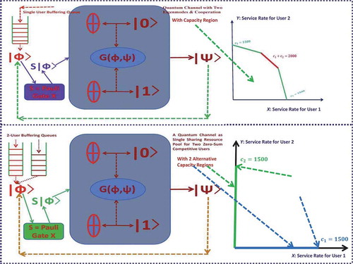
Thus, we will omit the related pool index $v$ in our discussion of this subsection for simplicity. Related to this system, two cases will be concerned as shown in Figure 10. The first case is corresponding to the upper graph in Figure 10, where only single user is allowed. However, we can pretend to allocate the user’s arrival packets into two separate storage buffers with certain proportions as in the lower graph of Figure 10. In this case, we are interested in the issue concerning the rate (i.e. power) resource allocation cooperatively between the two eigenmodes inside the quantum computer. More precisely, in Figure 4, we take $V=1$ and $J=2$ (i.e. we think of the single-pool system with two eigenmodes as a two user MIMO channel). Furthermore, we assume that the state space of the FS-CTMC $\alpha (t)$ defined in Subsection 2.2 consists only of a single state 1 (i.e. $\alpha (t)\equiv 1$ for all $t\in [0,\mathrm{\infty })$). In an MIMO wireless environment, such a case is corresponding to the so-called pseudo static channels (see, e.g. Dai [24] and Bhardwaj et al. [41]). Then, the capacity region denoted by $\mathcal{R}$ is assumed to be a non-degenerate convex one confined by five boundary lines including the two ones on $x$-axis and $y$-axis as shown in the upper-right graph of Figure 10. The capacity upper bound of the region satisfies $c_1+c_2=2000$. This region is corresponding to a degenerate fixed MIMO wireless channel of the generally randomized one in Dai [24]. For each rate vector $c=(c_1,c_2)\in \mathcal{R}$, we take the utility functions for user 1 and user 2, respectively, by

(3.13) $U_1(q,c)=U_1(q_1,c_1)=q_{1}ln(c_1),U_2(q,c)=U_2(q_2,c_2)=-\frac{q_2^2}{c_2^2},$(3.13)

where, $ln(\cdot )$ is the logarithm function with the base $e$. Furthermore, the vector $q=(q_1,q_2)\in [0,\mathrm{\infty })\times [0,\mathrm{\infty })$ is a given queue length of 2-users and it corresponds to the queue length process $Q(t)$ defined in (2.16) at a particular time point. The utility functions $U_1$ and $U_2$ are called proportionally fair and minimal potential delay allocations respectively, which are widely used in the design of communication protocols (see, e.g. Ye and Yao [42]). Based on these utility functions, we can propose our rate-scheduling policy at each time point $t\in [0,\mathrm{\infty })$ by a Pareto maximal-utility Nash equilibrium point to the non-zero-sum game problem for the case of two eigenmode cooperation. This case is a special situation as studied in Dai [2] and hence we will omit the remaining details here. Nevertheless, in the following discussion, we will present our new findings in a zero-sum game case study or called the second case as shown in the lower graph of Figure 10, which also comes up in recent smart power and energy switching system, i.e. IoE (see, e.g. Artemis [11] and Dai [43]).

More precisely, in this second zero-sum game case, only a single user (either user 1 or user 2) is allowed to get into service at each time point $t\in [0,\mathrm{\infty })$. Furthermore, we suppose that the service capacity is already determined as shown in the lower graph of Figure 10, i.e. $c_1=1500$ for user $1$ and $c_2=1500$ for user $2$. Then, based on the above given utility functions, we can design our rate-scheduling policy at each time point $t\in [0,\mathrm{\infty })$ by a saddle point to the zero-sum game problem

(3.14) $\underset{c\in \mathcal{R}}{max}{U}_0(q,c),\underset{c\in \mathcal{R}}{max}{U}_j(q,c),\underset{c\in \mathcal{R}}{max}\left(-U_{2-j+1}(q,c)\right)$(3.14)

for each $j\in \{1,2\}$ and a fixed $q\in R_{+}^2$, where, $U_0(q,c)=U_1(q,c)+U_2(q,c)$ and $R_{+}^2=[0,\mathrm{\infty })\times [0,\mathrm{\infty })$. In other words, if $c^{\ast }=(c_1^{\ast },c_2^{\ast })$ with is a solution to the game problem in (3.14), we can conclude that

(3.15) $U_0(q,c^{\ast })\ge U_0(q,c)$(3.15)

for a fixed $q\in R_{+}^2$. Furthermore, for each $j\in \{1,2\}$,

(3.16) $U_j(q,c^{\ast })\ge U_j(q,c_{-j}^{\ast })\mathrm{w}\mathrm{i}\mathrm{t}\mathrm{h}{c}_{\cdot -1}^{\ast }=(c_j,c_{2-j+1}^{\ast }),$(3.16)

(3.17) $-U_{2-j+1}(q,c^{\ast })\ge -U_{2-j+1}(q,c_{-(2-j+1)}^{\ast })\mathrm{w}\mathrm{i}\mathrm{t}\mathrm{h}{c}_{\cdot -(2-j+1)}^{\ast }=(c_j^{\ast },c_{2-j+1}).$(3.17)

3.2.2. General capacity region

In our platform, the jobs in the $j$th queue for each $j\in \mathcal{J}$ can be served simultaneously by a random but at most $V_j$ ($\le V$) number of service pools at a given time point. It can be realized by processors-sharing techniques or through multiple users’ and antennas’ cooperation in MIMO wireless channels, i.e. base stations can perform joint beamforming and/or power control at a particular time period. Under this simultaneous service mechanism, the total service rate for the jth queue at the time point is the summation of the rates from all the pools possibly to serve the jth queue. For convenience, we index such pools by a subset $\mathcal{V}(j)$ of the set $\mathcal{V}$, i.e.

(3.18) $\mathcal{V}(j)\equiv \{v_{1j},...,v_{V_{j}j}\}\subseteq \mathcal{V},$(3.18)

where, $v_{lj}$ for each $l\in \{1,...,V_j\}$ indexes the $v_{lj}$th pool in $\mathcal{V}(j)$.

In the same way, a pool indexed by $v\in \mathcal{V}$ can possibly serve at most $J_v$ number of job classes indexed by a subset $\mathcal{V}(v)$ of the set $\mathcal{J}$, i.e.

(3.19) $\mathcal{J}(v)\equiv \{j_{v1},...,j_{v{J}_v}\}\subseteq \mathcal{J},$(3.19)

where, $j_{vl}$ for each $l\in \{1,...,J_v\}$ indexes the $j_{vl}$th job class in $\mathcal{J}(v)$. The pool $v$ is equipped with $J_v$ number of flexible parallel-servers with rate allocation vector

(3.20) $c_{v\cdot }(t)=(c_{j_{v1}}(t),...,c_{j_{v{J}_v}}(t))\prime ,$(3.20)

where, $c_{j_{vl}}(t)$ for each $l\in \{1,...,J_v\}$ is the assigned service rate to the $j_{vl}$th user at pool $v$ and time $t$. In the sequel, we will also denote the rate $c_{j_{vl}}(t)$ by $c_{vj}(t)$ for an index $j\in \mathcal{J}(v)$ that corresponds to the $l\in \{1,...,J_v\}$. The vector in (3.20) takes values in a capacity region ${\mathcal{R}}_v(\alpha (t))$ driven by the FS-CTMC $\alpha =\{\alpha (t),t\in [0,\mathrm{\infty })\}$.

Figure 11. A 3-user capacity set in $R_{+}^3$ for a cooperative MIMO wireless channel in the left graph. A degenerate 3-user capacity set in $R_{+}^3$ for a cloud-processors-sharing system in the right graph. The upper graph is adapted from Figure 8.

For each $i\in \mathcal{K}$ and $v\in \mathcal{V}$, the set ${\mathcal{R}}_v(i)$ is a convex region consisting of the origin and owns $L_v$ $(>J_v)$ boundary pieces (see, e.g. the left graph of Figure 11 is an example in Dai [24], the right graph of Figure 11 is an example of Ye and Yao [42], and the detailed explanations for these two graphs are presented at the end of this subsubsection). In the region, each point is defined according to the corresponding users, i.e. $x=(x_{j_{v1}},...,x_{j_{v{J}_v}})$. On the boundary of ${\mathcal{R}}_v(i)$ for each $i\in \mathcal{K}$, $J_v$ of them are $(J_v-1)$-dimensional linear facets along the coordinate axes. The other ones are located in the interior of $R_{+}^{J_v}$ and form the so-called capacity surface represented by ${\mathcal{O}}_v(i)$, which has $B_v=L_v-J_v(>0)$ linear or smooth curved facets $h_{vk}(c_{v\cdot },i)$ on $R_{+}^{J_v}$ for $k\in {\mathcal{U}}_v\equiv \{1,2,...,B_v\}$, i.e.

(3.21) ${\mathcal{R}}_v(i)\equiv \left\{c_{v\cdot }\in R_{+}^{J_v}:h_{vk}(c_{v\cdot },i)\le 0,k\in {\mathcal{U}}_v\right\}.$(3.21)

If let $C_{U_v}(i)$ denote the sum capacity upper bound for ${\mathcal{R}}_v(i)$, the facet in the centre of ${\mathcal{O}}_v(i)$ is linear and is assumed to be a non-degenerate $(J_v-1)$-dimensional region. More precisely, it can be expressed by

(3.22) $h_{v{k}_{U_v}}(c_{v\cdot },i)=\sum _{j\in \mathcal{J}(v)}{c}_j-C_{U_v}(i),$(3.22)

where, $k_{U_v}\in {\mathcal{U}}_v$ is the index corresponding to $C_{U_v}(i)$. Furthermore, we assume that any one of the $J_v$ linear facets along the coordinate axes forms an $(J_v-1)$-user capacity region associated with a particular group of $J_v-1$ users when the queue corresponding to the other user is empty. By the same way, we can interpret the $(J_v-l)$-user capacity region for each $l\in \{2,...,J_v-1\}$.

In the allocation of the service resources over the capacity regions to different users, we adopt the so-called head of line service discipline. In other words, the service goes to the packet at the head of the line for a serving queue where packets are stored in the order of their arrivals. The service rates are determined through a function of the environmental state and the number of packets in each of the queues. For each state $i\in \mathcal{K}$ and a given queue length vector $q=(q_1,...,q_J)\prime$, let ${\mathrm{\Lambda }}_{\cdot j}(q,i)$ for each $j\in \mathcal{J}$ denote the rate vector (in bps) of serving the $j$th queue at all its possible service pools, i.e.

(3.23) ${\mathrm{\Lambda }}_{\cdot j}(q,i)=c_{\cdot j}^{\mathcal{Q}(q)}(i)=(c_{v_{1j}}^{\mathcal{Q}(q)}(i),...,c_{v_{V_{j}j}}^{\mathcal{Q}(q)}(i)),$(3.23)

where,

(3.24) $\mathcal{Q}(q)\equiv \{j\in \mathcal{J},q_j=0\}.$(3.24)

In the meanwhile, let ${\mathrm{\Lambda }}_{v\cdot }(q,i)$ for each $v\in \mathcal{V}$ denote the rate vector for all the users possibly served at service pool $v$, i.e.

(3.25) ${\mathrm{\Lambda }}_{v\cdot }(q,i)=c_{v\cdot }^{\mathcal{Q}(q)}(i)=(c_{j_{v1}}^{\mathcal{Q}(q)}(i),...,c_{j_{v{J}_v}}^{\mathcal{Q}(q)}(i)).$(3.25)

Obviously, if the pool index $v_{lj}\in \mathcal{V}(j)$ for an integer $l\in \{1,...,V_j\}$ with $j\in \mathcal{J}$, we have that $c_{v_{lj}}^{\mathcal{Q}(q)}(i)=c_j^{\mathcal{Q}(q)}(i).$ Thus, for each $j\in \mathcal{J}$, the total rate used in (2.17) can be expressed as

(3.26) ${\mathrm{\Lambda }}_j(Q(s),\alpha (s))=\sum _{v\in \mathcal{V}(j)}{c}_{vj}^{\mathcal{Q}(Q(s))}(\alpha (s)).$(3.26)

Finally, we impose the convention that an empty queue should not be served. Thus, for each $v\in \mathcal{V}$ and $\mathcal{Q}\subseteq \mathcal{J}$ (e.g. a set as given by (3.24)), we can define

(3.27) $c_{j_{vl}}^{\mathcal{Q}}(i)\equiv \left\{\begin{array}{cc}=0& \mathrm{i}\mathrm{f}{j}_{vl}\in \mathcal{Q}\mathrm{w}\mathrm{i}\mathrm{t}\mathrm{h}l\in \{1,...,J_v\},\\ >0& \mathrm{i}\mathrm{f}{j}_{vl}\notin \mathcal{Q}\mathrm{w}\mathrm{i}\mathrm{t}\mathrm{h}l\in \{1,...,J_v\},\end{array}\right.$(3.27)

(3.28) $c_{vj}^{\mathcal{Q}}(i)\equiv c_{j_{vl}}^{\mathcal{Q}}(i)\mathrm{f}\mathrm{o}\mathrm{r}\mathrm{s}\mathrm{o}\mathrm{m}\mathrm{e}j\in \mathcal{J}(v)\mathrm{c}\mathrm{o}\mathrm{r}\mathrm{r}\mathrm{e}\mathrm{s}\mathrm{p}\mathrm{o}\mathrm{n}\mathrm{d}\mathrm{i}\mathrm{n}\mathrm{g}\mathrm{t}\mathrm{o}\mathrm{e}\mathrm{a}\mathrm{c}\mathrm{h}l\in \{1,...,J_v\},$(3.28)

(3.29) $F_Q^v(i)\equiv \{x\in {\mathcal{R}}_v(i):x_{j_{vl}}=0\mathrm{f}\mathrm{o}\mathrm{r}\mathrm{a}\mathrm{l}\mathrm{l}{j}_{vl}\in \mathcal{Q}\mathrm{w}\mathrm{i}\mathrm{t}\mathrm{h}l\in \{1,...,J_v\}\}.$(3.29)

Hence, for all $\mathcal{Q}$ such that $\mathrm{\varnothing }\underset{\ne }{\subset }\mathcal{Q}\subseteq J(v)$ corresponding to each $v\in \mathcal{V}$, if $c_{v\cdot }^{\mathcal{Q}}(i)$ is on the boundaries of the capacity region ${\mathcal{R}}_v(i)$, we have the following observation that

(3.30) $\sum _{j\in \mathcal{J}(v)}{c}_{vj}^{\mathrm{\varnothing }}(i)\ge \sum _{j\in \mathcal{J}(v)}{c}_{vj}^{\mathcal{Q}}(i),$(3.30)

(3.31) $\sum _{j\in \mathcal{J}(v)\mathrm{\setminus }\mathcal{Q}}{c}_{vj}^{\mathrm{\varnothing }}(i)\le \sum _{j\in \mathcal{J}(v)\mathrm{\setminus }\mathcal{Q}}{c}_{vj}^{\mathcal{Q}}(i),$(3.31)

where, $c_{v\cdot }^{\mathrm{\varnothing }}(i)\in {\mathcal{O}}_v(i)$ and $\mathrm{\varnothing }$ denotes the empty set.

Typical examples of our capacity region include those for $J$-user MIMO multiple access uplink and broadcast downlink wireless channels, two-way or future quantum communication channels, and $J$-user cloud-processors-sharing centres or links (see, e.g. Goldsmith et al. [38], Jindal [44], Dai [24], Shapiro et al. [45], Childs et al. [46], Ye and Yao [42]). In a cooperative wireless channel, the inequalities in (3.30) and (3.31) are both strict, which leads to a capacity region (e.g. with three users) as displayed in the left graph of Figure 11. Note that, in this three-user case, there are 3 linear facets along the coordinate axes and 13 linear or smooth curved facets on the capacity surface. Furthermore, for such an MIMO channel, the capacity region reflects the cooperation property that the maximum of the sum of the rates is achieved only when all of the queues are non-empty. However, in a general cloud-processors-sharing service system, the equalities in (3.30) and (3.31) may be both true, which leads to a degenerate capacity region as shown in the right graph of Figure 11.

3.2.3. The DCNN and game-competition based scheduling policy

To integrate the decision processes in cognitive radio (see, e.g. Akyildiz et al. and Haykin [13]), FinTech, IoE (see, e.g. Artemis [11] and Dai [43]), etc. into our AI based scheduling system, we classify the users into two types (e.g. primary users and secondary users as in the cognitive radio). In this situation, we first need to smartly select the users (e.g. among the secondary users) to be served, i.e. at each time point and for each pool $v$, we smartly choose a set $\mathcal{M}(i,v)\equiv \{j_{v1}(i),...,j_{v{M}_v}(i)\}$ of users with $j_{vl}\in \mathcal{J}$ and $l\in \{1,...,M_v\}$ for a given $M_v\le J_v$ to get into service. Among these selected users, we need to dynamically realize the optimal and fair resource allocation. Therefore, we design a strategy by mixing a saddle point and a static Pareto maximal-utility Nash equilibrium policy myopically at each time point $t$ to a mixed zero-sum and non-zero-sum game problem for each state $i\in \mathcal{K}$ and a given queue length vector $q=(q_1,...,q_J)\prime$. The saddle point corresponds the users’ selection while the Pareto optimality represents the full utilization of resources in the whole game system and the Nash equilibrium represents the fairness to all the selected users. More precisely, in this game, there are $J$ users (players) corresponding to the $J$ queues and each of them has his own utility function $U_{vj}(q_j,c_{vj})$ with $j\in \mathcal{J}(v)$ and $v\in \mathcal{V}(j)$. The utility functions may also depend on some additional parameters such as prices. Nevertheless, in the current paper, we assume that they are pre-negotiated and are given. Every selected user chooses a policy to maximize his own utility function at each service pool $v$ while the summation of all the users’ utility functions and the summation of the utility functions corresponding to the selected users are also maximized. In other words, we can formulate the following generalized user-selection and resource-scheduling game problem by extending the one in Example 3.4,

(3.32) $\underset{c_{v\cdot }\in F_{\mathcal{Q}}^v(i)}{max}{U}_{00}(q,c)=U_{00}(q,c^{\ast }(i)),$(3.32)

(3.33) $\underset{c_{v\cdot }\in F_{\mathcal{Q}}^v(i)}{max}{U}_{0j}(q,c)=U_{0j}(q,c^{\ast }(i)),j\in \mathcal{M}(i,v)\cap (\mathcal{J}(v)\mathrm{\setminus }\mathcal{Q}(q)),$(3.33)

(3.34) $\underset{c_{v\cdot }\in F_{\mathcal{Q}}^v(i)}{max}(-U_{0j}(q,c))=-U_{0j}(q,c^{\ast }(i)),j\in (\mathcal{J}(v)\mathrm{\setminus }\mathcal{Q}(q))\mathrm{\setminus }\mathcal{M}(i,v))$(3.34)

while we have that

(3.35) $\underset{c_{v\cdot }\in F_{\mathcal{Q}}^v(i),j\in \mathcal{M}(i,v)\cap \left(\mathcal{J}(v)\mathrm{\setminus }\mathcal{Q}(q)\right)}{max}{U}_{vj}(q,c)=U_{vj}(q,c^{\ast }(i)),$(3.35)

(3.36) $\underset{c_{v\cdot }\in F_{\mathcal{Q}}^v(i),j\in \left(\mathcal{J}(v)\mathrm{\setminus }\mathcal{Q}(q)\right)\mathrm{\setminus }\mathcal{M}(i,v)}{max}(-U_{vj}(q,c))=-U_{vj}(q,c^{\ast }(i)).$(3.36)

Note that, the rate vector $c$ in (3.32)–(3.36) is given by

$c=((c_{j_{11}},\dots ,c_{j_{1J_1}}),\dots ,(c_{j_{V1}},\dots ,c_{j_{V{J}_V}}))$

and the objective functions are defined by

$U_{00}(q,c)=\sum _{v\in \mathcal{V}(j)}\sum _{j\in \mathcal{J}(v)\mathrm{\setminus }\mathcal{Q}(q)}{U}_{vj}(q_j,c_{vj}),$

$U_{0j}(q,c)=\sum _{v\in \mathcal{V}(j)}{U}_{vj}(q_j,c_{vj})\mathrm{f}\mathrm{o}\mathrm{r}\mathrm{e}\mathrm{a}\mathrm{c}\mathrm{h}j\in \mathcal{J}(v)\mathrm{\setminus }\mathcal{Q}(q),$

$U_{vj}(q,c)=U_{vj}(q_j,c_{vj})\mathrm{f}\mathrm{o}\mathrm{r}\mathrm{e}\mathrm{a}\mathrm{c}\mathrm{h}j\in \mathcal{J}(v)\mathrm{\setminus }\mathcal{Q}(q)\mathrm{a}\mathrm{n}\mathrm{d}v\in \mathcal{V}(j).$

Note that, the total utility function $U_{00}(q,c)$ does not have to be a constant (e.g. zero). In other words, the game is not necessarily a zero-sum one. Thus, by unifying the concepts of Nash equilibrium and Pareto optimality in Nash [47] and Rosen [48], we have the definition concerning a static Pareto maximal-utility Nash equilibrium policy myopically at a particular time point for the dynamic scheduling game as follows.

Definition 3.2 For each state $i\in \mathcal{K}$ and a queue length vector $q\in R_{+}^J$, the rate vector

$c^{\ast }(i)\in F_{\mathcal{Q}(q)}(i)\equiv F_{\mathcal{Q}(q)}^1(i)\times \dots \times F_{\mathcal{Q}(q)}^V(i)$

is called a mixed saddle-point and static Pareto maximal-utility Nash equilibrium policy to the mixed zero-sum and non-zero-sum game problem in (3.35) if, for each $j\in \mathcal{J}(v)\mathrm{\setminus }\mathcal{Q}(q)$ and any given $c(i)\in F_{\mathcal{Q}(q)}(i)$, we have that

(3.37) $U_{00}(q,c^{\ast }(i))\ge U_{00}(q,c(i)),$(3.37)

(3.38) $U_{vj}(q,c^{\ast }(i))\ge U_{vj}(q,c_{\cdot -j}^{\ast }(i))ifj\in \mathcal{M}(i,v)\cap (\mathcal{J}(v)\mathrm{\setminus }\mathcal{Q}(q)),v\in \{0\}\cup \mathcal{V}(j),$(3.38)

(3.39) $-U_{vj}(q,c^{\ast }(i))\ge -U_{vj}(q,c_{\cdot -j}^{\ast }(i))ifj\in (\mathcal{J}(v)\mathrm{\setminus }\mathcal{Q}(q))\mathrm{\setminus }\mathcal{M}(i,v),v\in \{0\}\cup \mathcal{V}(j),$(3.39)

(3.40) $c_{\cdot -j}^{\ast }(i)\equiv (c_{\cdot 1}^{\ast }(i),...,c_{\cdot j-1}^{\ast }(i),c_{\cdot j}(i),c_{\cdot j+1}^{\ast }(i),...,c_{\cdot J}^{\ast }(i)).$(3.40)

3.3. Identifying an RDRS model under the policy

In this subsection, we identify the exact expression of an RDRS model corresponding to the CNN and game-competition based AI scheduling policy designed in the previous subsection.

3.3.1. The obtained model by asymptotic approximation

To state our main theorem, we need to introduce another concept of the so-called mixed saddle point and static Pareto minimal-dual-cost Nash equilibrium policy myopically at a particular time point. In doing so, we formulate a minimal-dual-cost game problem corresponding to the maximal-utility game problem in (3.35). More precisely, for each given $i\in \mathcal{K}$, a rate vector $c\in \mathcal{R}(i)\equiv {\mathcal{R}}_1(i)\times ...\times {\mathcal{R}}_V(i)$, and a parameter $w\ge 0$, the problem can be stated as follows:

(3.41) $\underset{q_j\in R_{+}}{min}{C}_{00}(q,c),$(3.41)

(3.42) $\underset{q_j\in R_{+},j\in \mathcal{M}(i,v)\bigcap \left(\mathcal{C}(c)\bigcap \mathcal{J}(v)\right)}{min}{C}_{vj}(q,c),$(3.42)

(3.43) $\underset{q_j\in R_{+},j\in \left(\mathcal{C}(c)\bigcap \mathcal{J}(v)\right)\mathrm{\setminus }\mathcal{M}(i,v)}{min}(-C_{vj}(q,c))$(3.43)

subject to

$\sum _{j\in \mathcal{M}(i,v)\bigcap \mathcal{C}(c)}\frac{q_j}{{\mu }_j}\ge w,$

where, the cost function $C_{vj}(q,c)$ for each $j\in \mathcal{J}(v)$ and $v\in \{0\}\cup \mathcal{V}(j)$ is defined by

$C_{00}(q,c)=\sum _{v\in \mathcal{V}(j)}\sum _{j\in \mathcal{C}(c)\bigcap \mathcal{J}(v)}{C}_j(q_j,c_{vj}),$

$C_{0j}(q,c)=\sum _{v\in \mathcal{V}(j)}{C}_{vj}(q_j,c_{vj}),$

$C_{vj}(q,c)=C_{vj}(q_j,c_{vj})=\frac{1}{{\mu }_j}{\int }_0^{q_j}\frac{\mathrm{\partial }{U}_{vj}(u,c_{vj})}{\mathrm{\partial }{c}_{vj}}du\mathrm{f}\mathrm{o}\mathrm{r}j\in \mathcal{C}(c)\cap \mathcal{J}(v),v\in \mathcal{V}(j),$

and $\mathcal{C}(c)$ is an index set corresponding to the non-zero rates and non-empty queues, i.e.

$\mathcal{C}(c)\equiv \{j:c_{\cdot j}\ne 0\mathrm{c}\mathrm{o}\mathrm{m}\mathrm{p}\mathrm{o}\mathrm{n}\mathrm{e}\mathrm{n}\mathrm{t}\mathrm{w}\mathrm{i}\mathrm{s}\mathrm{e}\mathrm{w}\mathrm{i}\mathrm{t}\mathrm{h}j\in \mathcal{J}\}.$

In other words, when the environment is in state $i\in \mathcal{K}$, we try to identify a queue state $q$ corresponding to a given $c\in \mathcal{R}(i)$ and a given parameter $w\ge 0$ such that the individual user’s dual-costs and the total dual-cost over the system are all minimized at the same time while the (average) workload meets or exceeds $w$. In addition, the total dual-cost function $U_{00}(q,c)$ does not have to be a constant. Then, we have the following definition.

Definition 3.3 For each state $i\in \mathcal{K}$ and a rate vector $c(i)\in \mathcal{R}(i)$, the queue length vector $q^{\ast }\in R_{+}^J$ with $q_j^{\ast }=0$ if $j\in \mathcal{J}\mathrm{\setminus }\mathcal{C}(c)$ is called a mixed saddle point and static Pareto minimal-dual-cost Nash equilibrium policy to the mixed zero-sum and non-zero-sum game problem in (3.42) if, for each $j\in \mathcal{C}(c)$, $v\in \{0\}\cup \mathcal{V}$, and any given $q\in R_{+}^J$ with $q_j=0$ when $j\in \mathcal{J}\mathrm{\setminus }\mathcal{C}(c)$, we have that

(3.44) ${\mathcal{C}}_{00}(q^{\ast },c(i))\le {\mathcal{C}}_{00}(q,c(i)),$(3.44)

(3.45) ${\mathcal{C}}_{vj}(q^{\ast },c(i))\le {\mathcal{C}}_{vj}(q_{-j}^{\ast },c(i))ifj\in \mathcal{M}(i,v)\cap (\mathcal{C}(c)\cap \mathcal{J}(v)),$(3.45)

(3.46) $-{\mathcal{C}}_{vj}(q^{\ast },c(i))\le -{\mathcal{C}}_{vj}(q_{-j}^{\ast },c(i))ifj\in (\mathcal{C}(c)\mathcal{J}(v))\mathrm{\setminus }\mathcal{M}(i,v),$(3.46)

(3.47) $q_{-j}^{\ast }\equiv (q_1^{\ast },...,q_{j-1}^{\ast },q_j,q_{j+1}^{\ast },...,q_J^{\ast }).$(3.47)

Based on Definition 3.3 and the concept concerning the asymptotic optimality widely used in heavy traffic analysis (see, e.g. Ye and Yao [42], Dai [24]), we can develop some new concept about the asymptotic Pareto minimal-dual-cost Nash equilibrium policy as follows.

Definition 3.4 Let ${\hat{Q}}^{G,r}(\cdot )$ and ${\hat{W}}^{G,r}(\cdot )$ denote the diffusion-scaled queue length and workload processes respectively under an arbitrarily feasible rate scheduling policy $G$. A process $\hat{Q}(\cdot )$ is called a mixed asymptotic saddle point and Pareto minimal-dual-cost Nash equilibrium policy globally over the whole time horizon if

$\underset{r\to \mathrm{\infty }}{lim\mathrm{i}\mathrm{n}\mathrm{f}}{C}_{00}({\hat{Q}}^{r,G}(t),{\rho }_j(\alpha (t)))\ge C_{00}(\hat{Q}(t),{\rho }_j(\alpha (t))),$

$\underset{r\to \mathrm{\infty }}{lim\mathrm{i}\mathrm{n}\mathrm{f}}{\mathcal{C}}_{vj}({\hat{Q}}_{-j}^{r,G}(t),{\rho }_j(\alpha (t)))\ge {\mathcal{C}}_{vj}(\hat{Q}(t),{\rho }_j(\alpha (t))),j\in \mathcal{M}(\alpha (t),v,t)\cap (\mathcal{C}(c)\cap \mathcal{J}(v)),$

$\underset{r\to \mathrm{\infty }}{lim\mathrm{i}\mathrm{n}\mathrm{f}}(-{\mathcal{C}}_{vj}({\hat{Q}}_{-j}^{r,G}(t),{\rho }_j(\alpha (t))))\ge -{\mathcal{C}}_{vj}(\hat{Q}(t),{\rho }_j(\alpha (t))),j\in (\mathcal{C}(c)\cap \mathcal{J}(v))\mathrm{\setminus }\mathcal{M}(\alpha (t),v,t)$

for any $t\ge 0$, $v\in \{0\}\cup \mathcal{V}(j)$, and

(3.48) ${\hat{Q}}_{-j}^{r,G}(t)=({\hat{Q}}_1(t),...,{\hat{Q}}_j^{r,G}(t),...,{\hat{Q}}_J(t)).$(3.48)

Now, let $q^{\ast }(w,\rho (i))$ be the mixed saddle point and Pareto minimal-dual-cost Nash equilibrium policy to the game problem in (3.42) with respect to each given $w$ and $i\in \mathcal{K}$ at time $t$. Then, our main theorem can be presented as follows.

Theorem 3.1 For the game scheduling policy determined by (3.35) with $Q^r(0)=0$ and conditions (4.7) – (4.12) (that will be detailed in Section 4), the sequence of $2$-tuple processes converges jointly in distribution, i.e.

(3.49) $({\hat{Q}}^r(\cdot ),{\hat{W}}^r(\cdot ))\Rightarrow (\hat{Q}(\cdot ),\hat{W}(\cdot ))alongr\in \mathcal{R}.$(3.49)

Furthermore, the limit queue length $\hat{Q}(\cdot )$ and total workload $\hat{W}(\cdot )$ have the relationship

(3.50) $\hat{Q}(t)=q^{\ast }(\hat{W}(t),\rho (\alpha (t))),$(3.50)

where, $\hat{W}(\cdot )$ is a $1$-dimensional RDRS in strong sense with

(3.51) $b(i,t)=\sum _{j\in {\bigcup }_{v\in \mathcal{V}}\mathcal{M}(i,v,t)}\frac{{\theta }_j(i)}{{\mu }_j},$(3.51)

(3.52) ${\sigma }^E(t)={\sigma }^S(t)=\left({\hat{\sigma }}_1(t),...,{\hat{\sigma }}_J(t)\right),$(3.52)

${\hat{\sigma }}_j(t)=\left\{\begin{array}{cc}\frac{1}{{\mu }_j}& ifj\in {\bigcup }_{v\in \mathcal{V}}\mathcal{M}(i,v,t),\\ 0& otherwise,\end{array}\right.$

(3.53) $R(i,t)=1$(3.53)

for $t\in [0,\mathrm{\infty })$ and some constant ${\theta }_j(i)$ for each $j\in {\bigcup }_{v\in \mathcal{V}}\mathcal{M}(i,v,t)$. In addition, there is a common supporting probability space, under which and with probability one, the limit queue length $\hat{Q}(\cdot )$ is an asymptotic mixed saddle point and Pareto minimal-dual-cost Nash equilibrium policy globally over time interval $[0,\mathrm{\infty })$. Finally, the limit workload $\hat{W}(\cdot )$ is also asymptotic minimal in the sense that

(3.54) $\underset{r\to \mathrm{\infty }}{liminf}{\hat{W}}^{r,G}(t)\ge \hat{W}(t).$(3.54)

Note that, the process $({\hat{Q}}^r(\cdot ),{\hat{W}}^r(\cdot ))$ in (3.49) is directly corresponding to the physical queueing process of $n$-quibt quantum data packets as defined in Subsection 2.2. However, the diffusive approximation limit process $(\hat{Q}(\cdot ),\hat{W}(\cdot ))$ is a continuous one in both time and space. Based on the $n$-qubit quantum computing myopically at each time point, it can be used as an approximating model to measure the system performance in the macro-flow level. Furthermore, due to the zero-sum and non-zero-sum two level competition involved, our current results are different from those in Dai [24], especially, the drift and diffusion coefficients presented in (3.51) and (3.52), respectively. The proof of Theorem 3.1 will be provided in Subsection 4.2. Instead, in the following subsection, we first present a simulation case study that based on a simulation procedure proposed for the RDRS in the theorem. More precisely, for a constant $T\in [0,\mathrm{\infty })$, we divide the interval $[0,T]$ equally into $n$ subintervals $\{[t_i,t_{i+1}],i\in \{0,1,...,n-1\}\}$ with $t_0=0$, $t_n=T$, and $\mathrm{\Delta }{t}_i=t_{i+1}-t_i=\frac{T}{n}$. Furthermore, let

(3.55) $\mathrm{\Delta }F(t_i)\equiv F(t_i)-F(t_{i-1})$(3.55)

for each process $F(\cdot )\in \{B^E(\cdot ),B^S(\cdot ),\hat{W}(\cdot ),\hat{Y}(\cdot )\}$. Then, we can develop an iterative procedure similar to Simulation Procedure 3.1 in Dai [2] to simulate the RDRS model derived in Theorem 3.1.

3.4. A simulation case study via RDRS model

In this subsection, we consider a single-pool system with two-users as presented in Subsubsection 3.2.1 and hence will omit all the related pool index $v$ for simplicity. Note that, in a corresponding real-world system, the parameter vector $q$ in (3.14) is the randomly evolving queue length process $Q(t)$ in (2.16). Furthermore, it is our concern about how to use the RDRS performance model in Definition 3.1 to evaluate the effectiveness of our designed myopic service policies for the scheduling example in Subsubsection 3.2.1 globally over the whole time horizon $[0,\mathrm{\infty })$. As mentioned in Subsubsection 3.2.1, the effectiveness of the myopic non-zero-sum game based policy for the case in the upper graph of Figure 10 has been numerically justified in Dai [2]. Thus, in this subsection, we numerically illustrate the effectiveness of the myopic zero-sum game policy designed in (3.14) for the case in the lower graph of Figure 10. In this case, there are two competing users: user 1 and user 2 with utility functions $U_1(q,c)$ and $U_2(q,c)$, respectively. They try to get into the quantum computing service channel through competition according to the policy in (3.14), i.e. only one user can get access to the channel through bids reflected in their utility functions at each particular time point as shown in Figure 12.

Figure 12. An illustration of simulation case study concerning its importance and applications.

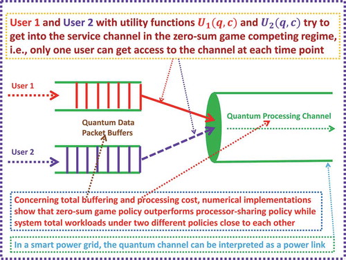
Therefore, our main task in this subsection is to apply the zero-sum game policy in (3.14) to conduct numerical experiments with computational results as displayed in Figure 9. From the figure, we can see that our policy outperforms processor-sharing policy in terms of total buffering and processing costs while the system total workloads under two different policies close to each other. It is worth to point out that our zero-sum game scheduling policy implemented in this section is a generic one. Besides the application in quantum computation, it also has the importance in other real-world problems such as smart power grid scheduling as shown in Figure 12.

To illustrate our numerical implementations, we first identify the associated dual-cost functions $C_j(q,c)$ as defined in (3.42) with $j\in \{1,2\}$ for corresponding $U_j(q,c)$ given in (3.13) . More precisely,

(3.56) $C_1(q_1,c_1)=\frac{1}{{\mu }_1}{\int }_0^{q_1}\frac{\mathrm{\partial }{U}_1(u,c_1)}{\mathrm{\partial }{c}_1}du=\frac{q_1^2}{2{\mu }_1{c}_1},$(3.56)

(3.57) $C_2(q_2,c_2)=\frac{1}{{\mu }_2}{\int }_0^{q_2}\frac{\mathrm{\partial }{U}_2(u,c_2)}{\mathrm{\partial }{c}_2}du=\frac{2q_2^3}{3{\mu }_2{c}_2^3},$(3.57)

where $1/{\mu }_j$ with $j\in \{1,2\}$ are average packet lengths corresponding the two users as explained just after the equation in (2.14) . Then, we can formulate the corresponding minimal dual-cost zero-sum game problem as

(3.58) $\underset{q\in [w{\mu }_1,\mathrm{\infty })\times [w{\mu }_2,\mathrm{\infty })}{min}{C}_0(q,c),\underset{q\in [w{\mu }_j,\mathrm{\infty })}{min}{C}_j(q_j,c_j),\underset{q\in [w{\mu }_{3-j},\mathrm{\infty })}{min}(-C_{3-j}(q_{3-j},c_{3-j})).$(3.58)

for a fixed constant $w>0$, a fixed $c\in \mathcal{R}$, and all $j\in \{0,1,2\}$ with $C_0(q,c)=$ $C_1(q,c)+C_2(q,c)$. Note that, both $C_j(q_j,c_j)$ for $j\in \{1,2\}$ are strictly increasing in terms of $q_j$. Thus, a dual-cost saddle point can be expressed as follows

(3.59) $q_j^{\ast }=\left\{\begin{array}{cc}w{\mu }_j& \mathrm{i}\mathrm{f}{C}_j(w{\mu }_j,c_j)\le C_{3-j}(w{\mu }_{3-j},c_{3-j}),\\ 0& \mathrm{o}\mathrm{t}\mathrm{h}\mathrm{e}\mathrm{r}\mathrm{w}\mathrm{i}\mathrm{s}\mathrm{e}.\end{array}\right.$(3.59)

In other words, for any $q\in [w{\mu }_1,\mathrm{\infty })\times [w{\mu }_2,\mathrm{\infty })$, we have

(3.60) $C_0(q^{\ast },c)\le C_0(q,c),$(3.60)

(3.61) $C_j(q^{\ast },c)\le C_j(q_{-j}^{\ast },c)\mathrm{w}\mathrm{i}\mathrm{t}\mathrm{h}{q}_{-j}^{\ast }=(q_j,q_{3-j}^{\ast }),$(3.61)

(3.62) $-C_{3-j}(q^{\ast },c)\le -C_{3-j}(q_{-(3-j)}^{\ast },c)\mathrm{w}\mathrm{i}\mathrm{t}\mathrm{h}{q}_{-(3-j)}^{\ast }=(q_j^{\ast },q_{3-j}).$(3.62)

Furthermore, for the purpose of comparison, we also design an alternative scheduling policy associated with a uniformly generated random number $u$ over interval $[0,1]$ as follows,

(3.63) $q_j^{\ast }=\left\{\begin{array}{cc}w{\mu }_j& \mathrm{i}\mathrm{f}u\in [0,1/2],\\ 0& \mathrm{i}\mathrm{f}u\in [(1/2,1],\end{array}\right.q_{3-j}^{\ast }=\left\{\begin{array}{cc}0& \mathrm{i}\mathrm{f}u\in [0,1/2],\\ w{\mu }_{3-j}& \mathrm{i}\mathrm{f}u\in (1/2,1].\end{array}\right.$(3.63)

In addition, it follows from the inequalities in (3.60)–(3.62) that the cost of a dual-cost game player $j$ with $j\in \{1,2\}$ cannot be reduced if he unilaterally changes his bid’s policy $q_j$.

Based on these properties, we can illustrate the effectiveness of our designed policy by the dual-cost game problem in (3.58). More precisely, in our Theorem 3.1 and the following RDRS modelling demonstration in Subsection 4, we have the claim that the physical workload $W(t)$ in (2.18) for this single pool case can indeed be modelled by an RDRS as introduced in Definition 0.2 if certain load balance condition holds. Moreover, $W(t)$ is asymptotically minimal at any time $t\in [0,\mathrm{\infty })$ almost surely along any sample path in some supporting probability space. In the meanwhile, the queue length process $Q(t)$ in (2.16) is also minimized in the sense that it is asymptotically dual-cost saddle point process given by $Q(t)=q^{\ast }(W(t))$ where $q^{\ast }(w)$ is given in (3.59). Note that, for this example, it follows from Theorem 3.1 that the coefficients of the 1-dimensional RDRS under our game-based scheduling policy for the physical workload process $\hat{W}$ can be denoted by

(3.64) $\hat{b}=\left\{\begin{array}{cc}\frac{{\theta }_j}{{\mu }_j}& \mathrm{i}\mathrm{f}{C}_j(w{\mu }_j,c_j)\le C_{3-j}(w{\mu }_{3-j},c_{3-j}),\\ \frac{{\theta }_{3-j}}{{\mu }_{3-j}}& \mathrm{o}\mathrm{t}\mathrm{h}\mathrm{e}\mathrm{r}\mathrm{w}\mathrm{i}\mathrm{s}\mathrm{e},\end{array}\right.{\hat{\sigma }}^E={\hat{\sigma }}^S=\left({\hat{\sigma }}_1,{\hat{\sigma }}_2\right),\hat{R}=1.$(3.64)

where, for $j\in \{1,2\}$, we have that

(3.65) ${\hat{\sigma }}_j=\left\{\begin{array}{cc}\frac{1}{{\mu }_j}& \mathrm{i}\mathrm{f}{C}_j(w{\mu }_j,c_j)\le C_{3-j}(w{\mu }_{3-j},c_{3-j}),\\ 0& \mathrm{o}\mathrm{t}\mathrm{h}\mathrm{e}\mathrm{r}\mathrm{w}\mathrm{i}\mathrm{s}\mathrm{e}.\end{array}\right.$(3.65)

Thus, by the $1$-dimensional RDRS corresponding to (3.64) and (3.65) and the saddle point policy $q^{\ast }$ in (3.59), we can apply the iterative formula (called Simulation Procedure $3.1$ in Dai [2]) to conduct our workload based numerical simulation. Here, we point out that all the processes related to the workload processes will be covered with a ‘hat’.

Next, based on the given parameters as shown in the bottom of Figure 9, we present the simulation results for our case study as summarized in the $12$ graphs of the figure. In this example, the number $N$ of simulation iterative times is 96,000. The simulation time interval is $[0,T]$ with $T=30$ and it is divided into n = 10,000 subintervals. Furthermore, all the ‘simulated means’ used in the graphs are in the average sense, e.g. the simulated mean workload is given by

(3.66) $E\left[\hat{W}(t_i)\right]=\frac{1}{N}\sum _{j=1}^N\hat{W}({\omega }_j,t_i),$(3.66)

where, ${\omega }_j$ denotes the used $j$th sample paths of $\hat{W}(\cdot )$ and $t_i\in [0,30]$ with $i\in \{0,1,...,10000\}$ and $t_0=0$ is the time index. Note that, in Figure 9, we give the performance evaluation and comparisons with respect to the workload process $\hat{W}(\cdot )$. The red curve displayed in the first graph of the left column is the simulated mean workload function with respect to time point $t_i$ under the saddle point policy. The result presented in the second graph of this column shows the difference between the simulated mean workload directly through the RDRS model associated with the coefficients in (3.64) and (3.65) and the corresponding one obtained by the saddle point policy displayed in (3.59), i.e.

(3.67) $E[\hat{W}(t_i)]-E[{\hat{W}}^{\ast }(t_i)].$(3.67)

Based on the curves in this graph, we can observe that the two workload processes are quite consistent. The curves shown in the third graph of this column are the decision paths of the saddle point policy given in (3.59) for the two users. The curve in the fourth graph of this column displays the difference of the workloads under the saddle point policy in (3.59) and the arbitrarily selected alternative policy in (3.63). Actually, under this alternative policy, the corresponding system is a single-server polling system with two job classes, the workload process can also be approximated by the RDRS model when our load balance condition is applied (see, e.g. Coffman et al. [49]). Thus, from the workload perspective, the workloads under these two scheduling policies should be close to each other as shown in the graph. However, if we conduct one more deep-level study concerning the system total cost as displayed in the red curve of the fourth graph on the second column, we see that our saddle point policy outperforms the alternative one. In this graph, the other two curves are the errors corresponding to different users. The curves in the first graph of the second column display the decision paths of the alternative policy. The curve in the second graph of this column presents the simulated mean total cost under saddle point policy. The curves in the third graph of this column state the costs for different users under the saddle point policy. The curves in the graphs of the third column display the evolutions of queueing lengths for different users and their comparisons under the saddle point policy and the alternative policy.

4. RDRS modelling demonstration

In this section, we demonstrate the RDRS modelling presented in Theorem 3.1.

4.1. The conditions and assumptions

The utility functions can be either simply taken as the well-known proportionally fair and minimal potential delay allocations as used in (3.13) for Example 3.4 or generally taken such that the existence of a mixed saddle point and Pareto maximal-utility Nash equilibrium policy to the game problem in (3.35) is guaranteed. More precisely, we can suppose that $U_{vj}(q_j,c_{vj})$ for each $j\in \mathcal{J}(v)$ and $v\in \mathcal{V}(j)$ is defined on $R_{+}^J$. It is second-order differentiable and satisfies

(4.1) $U_{vj}(0,c_{vj})=0,$(4.1)

(4.2) $U_{vj}(q_j,c_{vj})={\mathrm{\Phi }}_{vj}(q_j){\mathrm{\Psi }}_v(c_{vj})\mathrm{i}\mathrm{s}\mathrm{s}\mathrm{t}\mathrm{r}\mathrm{i}\mathrm{c}\mathrm{t}\mathrm{l}\mathrm{y}\mathrm{i}\mathrm{n}\mathrm{c}\mathrm{r}\mathrm{e}\mathrm{a}\mathrm{s}\mathrm{i}\mathrm{n}\mathrm{g}\mathrm{a}\mathrm{n}\mathrm{d}\mathrm{c}\mathrm{o}\mathrm{n}\mathrm{c}\mathrm{a}\mathrm{v}\mathrm{e}\mathrm{i}\mathrm{n}{c}_{vj}\mathrm{f}\mathrm{o}\mathrm{r}{q}_j>0,$(4.2)

(4.3) ${\mathrm{\Psi }}_v({\nu }_j{c}_{vj})={\mathrm{\Psi }}_v({\nu }_j){\mathrm{\Psi }}_v(c_{vj})\mathrm{o}\mathrm{r}{\mathrm{\Psi }}_v({\nu }_j{c}_{vj})={\mathrm{\Psi }}_v({\nu }_j)+{\mathrm{\Psi }}_v(c_{vj})\mathrm{f}\mathrm{o}\mathrm{r}\mathrm{c}\mathrm{o}\mathrm{n}\mathrm{s}\mathrm{t}\mathrm{a}\mathrm{n}\mathrm{t}{\nu }_j\ge 0,$(4.3)

(4.4) $\frac{\mathrm{\partial }{U}_{vj}(q_j,c_{vj})}{\mathrm{\partial }{c}_{vj}}\mathrm{i}\mathrm{s}\mathrm{s}\mathrm{t}\mathrm{r}\mathrm{i}\mathrm{c}\mathrm{t}\mathrm{l}\mathrm{y}\mathrm{i}\mathrm{n}\mathrm{c}\mathrm{r}\mathrm{e}\mathrm{a}\mathrm{s}\mathrm{i}\mathrm{n}\mathrm{g}\mathrm{i}\mathrm{n}{q}_j\ge 0,$(4.4)

(4.5) $\frac{\mathrm{\partial }{U}_{vj}(0,c_{vj})}{\mathrm{\partial }{c}_{vj}}=0\mathrm{a}\mathrm{n}\mathrm{d}\underset{q_j\to \mathrm{\infty }}{lim}\frac{\mathrm{\partial }{U}_{vj}(q_j,c_{vj})}{\mathrm{\partial }{c}_{vj}}=+\mathrm{\infty }\mathrm{f}\mathrm{o}\mathrm{r}\mathrm{e}\mathrm{a}\mathrm{c}\mathrm{h}{c}_{vj}>0.$(4.5)

Furthermore, we assume that $\{U_{vj}(q_j,c_{vj}),j\in \mathcal{J}(v),v\in \mathcal{V}(j)\}$ satisfies the so-called radial homogeneity condition at each time point $t\in [0,\mathrm{\infty })$, i.e. for any scalar $a>0$, each $q>0$, $i\in \mathcal{K}$, $v\in \mathcal{V}$, and each $j_l\in \mathcal{M}(i,v,t)$ with corresponding $l\in \{1,...,M_v\}$, its Pareto maximal utility Nash equilibrium point for the game has the radial homogeneity

(4.6) $c_{v{j}_l}(aq,i)=c_{v{j}_l}(q,i).$(4.6)

In addition, we introduce a sequence of independent Markov processes indexed by $r\in \mathcal{R}$, i.e. $\{{\alpha }^r(\cdot ),r\in \mathcal{R}\}$. These systems all have the same basic structure as described in the last section except the arrival rates ${\lambda }_{j_l}^r(i)$ and the holding time rates ${\gamma }^r(i)$ for all $i\in \mathcal{K}$, which may vary with $r\in \mathcal{R}$. Here, we assume that they satisfy the heavy traffic condition

(4.7) $r\left({\lambda }_{j_l}^r(i)-{\lambda }_{j_l}(i)\right)m_{j_l}(i)\to {\theta }_{j_l}(i)\mathrm{a}\mathrm{s}r\to \mathrm{\infty },{\gamma }^r(i)=\frac{\gamma (i)}{r^2},$(4.7)

where, ${\theta }_{j_l}(i)\in R$ is some constant for each $i\in \mathcal{K}$. Moreover, we suppose that the nominal arrival rate ${\lambda }_{j_l}(i)$ is given by

(4.8) ${\lambda }_{j_l}(i)m_{j_l}(i)\equiv {\mu }_{j_l}{\rho }_{j_l}(i)$(4.8)

and ${\rho }_{j_l}(i)$ in (4.8) for $j_l\in \mathcal{M}(i,v,t)$ with $l\in \{1,...,M_v\}$ is the nominal throughput determined by

(4.9) ${\rho }_{j_l}(i)=\sum _{v\in V(j_l)}{\rho }_{v{j}_l}(i)\mathrm{a}\mathrm{n}\mathrm{d}{\rho }_{v{j}_l}(i)={\nu }_{v{j}_l}{\bar{\rho }}_{v{j}_l}(i)$(4.9)

with ${\rho }_{v\cdot }(i)\in {\mathcal{O}}_v(i)$ that is corresponding to the dimension $M_v$. In addition, ${\nu }_{v\cdot }$ and ${\bar{\rho }}_{v\cdot }(i)$ are an $J_v$-dimensional constant vector and a reference service rate vector, respectively, at service pool $v$, satisfying

(4.10) $\sum _{j_l\in \mathcal{M}(i,v,t)\bigcap \mathcal{J}(v)}{\nu }_{j_l}=J_v,{\nu }_{j_l}\ge 0\mathrm{a}\mathrm{r}\mathrm{e}\mathrm{c}\mathrm{o}\mathrm{n}\mathrm{s}\mathrm{t}\mathrm{a}\mathrm{n}\mathrm{t}\mathrm{s}\mathrm{f}\mathrm{o}\mathrm{r}\mathrm{a}\mathrm{l}\mathrm{l}{j}_l\in \mathcal{M}(i,v,t)\cap \mathcal{J}(v),$(4.10)

(4.11) $\sum _{j_l\in \mathcal{M}(i,v,t)\cap \mathcal{J}(v)}{\bar{\rho }}_{v{j}_l}(i)={\mathcal{C}}_{U_v}(i)\mathrm{a}\mathrm{n}\mathrm{d}{\bar{\rho }}_{v{j}_1}(i)={\bar{\rho }}_{v{j}_l}(i)\mathrm{f}\mathrm{o}\mathrm{r}\mathrm{a}\mathrm{l}\mathrm{l}{j}_l\in \mathcal{M}(i,v,t)\cap \mathcal{J}(v).$(4.11)

Remark 4.1 By (3.22), ${\bar{\rho }}_{v\cdot }(i)$ for each $i\in \mathcal{K}$ and $v\in \mathcal{V}(j_l)$ can indeed be selected, which satisfy the second condition in (4.11) . Thus, the nominal throughput $\rho (i)$ in (4.8) can be determined. One simple example that satisfies these conditions is to take ${\nu }_{v{j}_l}=1$ for all $j_l\in \mathcal{M}(i,v,t)\cap \mathcal{J}(v)$ and $v\in \mathcal{V}(j_l)$. Then, the conditions in (4.8) – (4.11) mean that the system manager hopes to maximally and fairly allocate capacity to all users. Furthermore, the system design parameters ${\lambda }_{j_l}(i)$ for all $j_l\in \mathcal{M}(i,v,t)\cap \mathcal{J}$ and each $i\in \mathcal{K}$ can be determined by (4.8) .

Now, we suppose that the inter-arrival time corresponding to the $k$th arriving job batch to the system indexed by $r\in \mathcal{R}$ is given by

(4.12) $u_{j_l}^r(k,i)=\frac{{\hat{u}}_{j_l}(k)}{{\lambda }_{j_l}^r(i)}\mathrm{f}\mathrm{o}\mathrm{r}\mathrm{e}\mathrm{a}\mathrm{c}\mathrm{h}{j}_l\in \mathcal{M}(i,v,t)\cap \mathcal{J},k\in \{1,2,...\},i\in \mathcal{K},$(4.12)

where, the ${\hat{u}}_{j_l}(k)$ does not depend on $r$ and $i$. Furthermore, it has mean one and finite squared coefficient of variation ${\alpha }_{j_l}^2$. In addition, the number of packets, $w_{j_l}(k)$, and the packet length $v_{j_l}(k)$ are assumed not to change with $r$. Furthermore, it follows from the heavy traffic condition in (4.7) for the $r$th environmental state process ${\alpha }^r(\cdot )$ with $r\in \mathcal{R}$ that ${\alpha }^r(r^2\cdot )$ and $\alpha (\cdot )$ are equal each other in distribution since they own the same generator matrix (see, e.g. the definition in pages 384–388 of Resnick [40]). Hence, in the sense of distribution, all of the systems indexed by $r\in \mathcal{R}$ in (3.1) share the same random environment over any time interval $[0,t]$.

4.2. Proof of theorem 3.1

First, from the second condition in (4.7), we know that the processes ${\alpha }^r(r^2\cdot )$ for each $r\in \mathcal{R}$ and $\alpha (\cdot )$ are equal in distribution. Thus, without loss of generality, we can suppose that

(4.13) ${\alpha }^r(r^{2}t)=\alpha (t)\mathrm{f}\mathrm{o}\mathrm{r}\mathrm{e}\mathrm{a}\mathrm{c}\mathrm{h}r\in \mathcal{R}\mathrm{a}\mathrm{n}\mathrm{d}t\in [0,\mathrm{\infty }).$(4.13)

Then, for each $j\in \mathcal{J}$, $r\in \mathcal{R}$ and by the radial homogeneity of $\mathrm{\Lambda }(q,i)$ of the policy in (4.6), we can define the fluid and diffusion scaled processes as follows,

(4.14) $E_j^r(\cdot )\equiv A_j^r(r^2\cdot ),$(4.14)

(4.15) ${\bar{T}}_j^r(\cdot )\equiv {\int }_0^{\cdot }{\mathrm{\Lambda }}_j\left({\bar{Q}}^r(s),\alpha (s),s\right)ds=\frac{1}{r^2}{T}_j^r(r^2\cdot ),$(4.15)

(4.16) ${\bar{Q}}_j^r(t)\equiv \frac{1}{r^2}{Q}_j^r(r^{2}t),$(4.16)

(4.17) ${\bar{E}}_j^r(t)\equiv \frac{1}{r^2}{E}_j^r(t),$(4.17)

(4.18) ${\bar{S}}_j^r(t)\equiv \frac{1}{r^2}{S}_j^r(r^{2}t).$(4.18)

Thus, by (2.16), (4.13), and the assumptions among arrival and service processes, we know that

(4.19) ${\hat{Q}}_j^r(\cdot )=\frac{1}{r}{E}_j^r(\cdot )-\frac{1}{r}{S}_j^r({\bar{T}}_j^r(\cdot )).$(4.19)

Furthermore, let

(4.20) ${\hat{E}}^r(\cdot )=({\hat{E}}_1^r(\cdot ),...,{\hat{E}}_J^r(\cdot ))\prime \mathrm{w}\mathrm{i}\mathrm{t}\mathrm{h}{\hat{E}}_j^r(\cdot )=\frac{1}{r}\left(A_j^r(r^2\cdot )-r^2{\bar{\lambda }}_j^r(\cdot )\right),$(4.20)

(4.21) ${\hat{S}}^r(\cdot )=({\hat{S}}_1^r(\cdot ),...,{\hat{S}}_J^r(\cdot ))\prime \mathrm{w}\mathrm{i}\mathrm{t}\mathrm{h}{\hat{S}}_j^r(\cdot )=\frac{1}{r}\left(S_j(r^2\cdot )-{\mu }_j{r}^2\cdot \right)$(4.21)

for each $j\in \mathcal{J}$ with

(4.22) ${\bar{\lambda }}_j^r(\cdot )\equiv {\int }_0^{\cdot }{m}_j(\alpha (s),s){\lambda }_j^r(\alpha (s),s)ds$(4.22)

$={\int }_0^{\cdot }{m}_j({\alpha }^r(r^{2}s),r^{2}s){\lambda }_j^r({\alpha }^r(r^{2}s),r^{2}s)ds$

$=\frac{1}{r^2}{\int }_0^{r^2\cdot }{m}_j({\alpha }^r(s),r^{2}s){\lambda }_j^r({\alpha }^r(s),r^{2}s)ds,$

and define

(4.23) ${\bar{\lambda }}^r(\cdot )={\left({\bar{\lambda }}_1^r(\cdot ),...,{\bar{\lambda }}_J^r(\cdot )\right)}^{\prime }.$(4.23)

In addition, we use ${\bar{Q}}^r(\cdot )$, ${\bar{E}}^r(\cdot )$, ${\bar{S}}^r(\cdot )$, and ${\bar{T}}^r(\cdot )$ to denote the corresponding vector processes. Then, corresponding to the processes in (4.14)–(4.19), we can define the following fluid limit related processes,

(4.24) ${\bar{Q}}_j(t)={\bar{Q}}_j(0)+{\bar{\lambda }}_j(t,{\zeta }_t(\cdot ))-{\mu }_j{\bar{T}}_j(t)\mathrm{f}\mathrm{o}\mathrm{r}\mathrm{e}\mathrm{a}\mathrm{c}\mathrm{h}j\in \mathcal{J},$(4.24)

(4.25) $\bar{\lambda }(t)={\left({\bar{\lambda }}_1(t),...,{\bar{\lambda }}_J(t)\right)}^{\prime },{\bar{\lambda }}_j(t)\equiv {\int }_0^t{\lambda }_j(\alpha (s),s)ds,$(4.25)

(4.26) ${\bar{T}}_j(t)={\int }_0^t{\bar{\mathrm{\Lambda }}}_j(\bar{Q}(s),\alpha (s),s)ds,$(4.26)

where, for each $i\in \mathcal{K}$ and $t\in [0,\mathrm{\infty })$, we have that

(4.27) ${\bar{\mathrm{\Lambda }}}_j(q,i,t)=\left\{\begin{array}{cc}{\mathrm{\Lambda }}_j(q,i,t)& \mathrm{i}\mathrm{f}{q}_j>0,j\in {\bigcup }_{v\in \mathcal{V}}\mathcal{M}(i,v,t),\\ {\rho }_j(i,t)& \mathrm{i}\mathrm{f}{q}_j>0,j\mathit{/}\subseteq {\bigcup }_{v\in \mathcal{V}}\mathcal{M}(i,v,t),\\ {\rho }_j(i,t)& \mathrm{i}\mathrm{f}{q}_j=0.\end{array}\right.$(4.27)

Then, we can present a lemma about the weak convergence to a stochastic fluid limit process under our DCNN and game-competition based scheduling strategy.

Lemma 4.1 Suppose that the initial queue length ${\bar{Q}}^r(0)\Rightarrow \bar{Q}(0)$ along $r\in \mathcal{R}$. Then, the joint convergence in distribution along a subsequence of $\mathcal{R}$ is true under the conditions required by Theorem 3.1,

(4.28) $\left({\bar{E}}^r(\cdot ),{\bar{S}}^r(\cdot ),{\bar{T}}^r(\cdot ),{\bar{Q}}^r(\cdot )\right)\Rightarrow \left(\bar{E}(\cdot ),\bar{S}(\cdot ),\bar{T}(\cdot ),\bar{Q}(\cdot )\right).$(4.28)

In addition, if $\bar{Q}(0)=0$, the convergence is true along the whole $\mathcal{R}$ and the limit satisfies

(4.29) $\bar{E}(\cdot )=\bar{\lambda }(\cdot ),\bar{S}(\cdot )=\mu (\cdot ),\bar{T}(\cdot )=\bar{c}(\cdot ),\bar{Q}(\cdot )=0,$(4.29)

where, $\bar{\lambda }(\cdot )$ is defined in (4.25), $\mu (\cdot )\equiv ({\mu }_1,...,{\mu }_J)\prime \cdot$, and $\bar{c}(\cdot )$ is defined by

(4.30) $\bar{c}(t)=\left({\bar{c}}_1(t),...,{\bar{c}}_J(t)\right)\prime \mathrm{a}\mathrm{n}\mathrm{d}{\bar{c}}_j(t)\equiv {\int }_0^t{\rho }_j(\alpha (s))dsforeachj\in \mathcal{J}.$(4.30)

Proof. By the proofs of Lemma 4.2 in Dai [2] and Lemma 7 in Dai [24], we only need to prove the claim that $\bar{Q}(\cdot )=0$ in (4.30) to be true for our current purpose. In fact, for each $i\in \mathcal{K}$ and $l\in \{1,...,M_v\}$, we define

(4.31) $\psi (q,i)\equiv \sum _{v\in \mathcal{V}}{\psi }_v(q,i)=\sum _{v\in \mathcal{V}}\sum _{j_l\in \mathcal{M}(i,v)\bigcap \mathcal{J}(v)}{C}_{v{j}_l}(q_{j_l},{\rho }_{v{j}_l}(i)).$(4.31)

It follows from the proof in Dai [24] that all the limits in (4.30) are absolutely continuous and differentiable at almost all $t\in (0,\mathrm{\infty })$. In other words, almost every $t\in (0,\mathrm{\infty })$ is a regular point of these limits. Hence, for each regular time $t\ge 0$ of $\bar{Q}(t)$ over time interval $({\tau }_{n-1},{\tau }_n)$ with a given $n\in \{1,2,...\}$, we have the observation that

(4.32) $\frac{d\psi (\bar{Q}(t),\alpha (t))}{dt}$(4.32)

$=\sum _{v\in \mathcal{V}}\sum _{j_l\in \mathcal{M}(i,v,t)\bigcap \mathcal{J}(v)}\left(\frac{d{\bar{Q}}_{j_l}(t)}{dt}\frac{\mathrm{\partial }{C}_{v{j}_l}({\bar{Q}}_{j_l}(t),{\rho }_{v{j}_l}(\alpha (t))}{\mathrm{\partial }{\bar{Q}}_{j_l}(t)}\right.$

$\left.+\frac{d{\rho }_{v{j}_l}(\alpha (t))}{dt}\frac{\mathrm{\partial }{C}_{v{j}_l}({\bar{Q}}_{j_l}(t),{\rho }_{v{j}_l}(\alpha (t))}{\mathrm{\partial }{\rho }_{v{j}_l}(\alpha (t))}\right)$

$=\sum _{v\in \mathcal{V}}\sum _{j_l\in \mathcal{M}(i,v,t)\bigcap \mathcal{J}(v)}\left({\rho }_{v{j}_l}(\alpha (t))-{\mathrm{\Lambda }}_{v{j}_l}(\bar{Q}(t),\alpha (t))\right)\frac{\mathrm{\partial }{U}_{vj}({\bar{Q}}_{j_l}(t),{\rho }_{v{j}_l}(\alpha (t)))}{\mathrm{\partial }{\rho }_{v{j}_l}(\alpha (t))}{I}_{\{{\bar{Q}}_{j_l}(t)>0\}}$

$\le 0,$

where, the second equality follows from the concavity of the utility functions and the fact that ${\mathrm{\Lambda }}_{vj}(\bar{Q}(t),\alpha (t))$ is the Pareto maximal Nash equilibrium policy to the utility-maximal game problem in (3.35) when the channel is in a particular state. Thus, for any given $n\in \{0,1,2,...\}$ and each $t\in [{\tau }_n,{\tau }_{n+1})$,

(4.33) $0\le \psi (\bar{Q}(t),\alpha (t))$(4.33)

$\le \psi (\bar{Q}({\tau }_n),\alpha ({\tau }_n))$

$=\sum _{v\in \mathcal{V}}\sum _{j_l\in \mathcal{M}(i,v,{\tau }_n)\bigcap \mathcal{J}(v)}\frac{1}{{\mu }_{j_l}}{\int }_0^{{\bar{Q}}_{j_l}({\tau }_n)}\frac{\mathrm{\partial }{U}_{v{j}_l}(u,{\rho }_{v{j}_l}(\alpha ({\tau }_n)))}{\mathrm{\partial }{C}_{v{j}_l}}du$

$=\sum _{v\in \mathcal{V}}\left(\frac{d{\psi }_v({\bar{\rho }}_{v{j}_1}(\alpha ({\tau }_n)))}{d{c}_{v{j}_1}}\right){\left(\frac{d{\psi }_v({\bar{\rho }}_{v{j}_1}(\alpha ({\tau }_{n-1})))}{d{c}_{v{j}_1}}\right)}^{-1}{\psi }_v(\bar{Q}({\tau }_n),\alpha ({\tau }_{n-1}))$

$\dots$

$\le \sum _{v\in \mathcal{V}}\left(\frac{d{\psi }_v({\bar{\rho }}_{v{j}_1}(\alpha ({\tau }_n)))}{d{c}_{v{j}_1}}\right){\left(\frac{d{\psi }_v({\bar{\rho }}_{v{j}_1}(\alpha ({\tau }_0)))}{d{c}_{v{j}_1}}\right)}^{-1}{\psi }_v(\bar{Q}(0),\alpha (0))$

$\le \kappa \psi (\bar{Q}(0),\alpha (0)),$

where, $\kappa$ is a positive constant given by

$\kappa =\underset{v\in \mathcal{V}}{max}\underset{i,j\in \mathcal{K}}{max}\left(\frac{d{\psi }_v({\bar{\rho }}_{v{j}_1}(i))}{d{c}_{v{j}_1}}\right){\left(\frac{d{\psi }_v({\bar{\rho }}_{v{j}_1}(j))}{d{c}_{v{j}_1}}\right)}^{-1}.$

Then, it follows from the fact in (4.34) that $\bar{Q}(t)=0$ for all $t\ge 0$. Hence, we complete the proof of the lemma. □

Finally, by considering a specific state $i\in \mathcal{K}$ and by the index way as used in proving Lemma 0.1, we can provide proofs for Lemma 4.3 to Lemma 4.5 in Dai [2] to be true in the current setting. Then, by applying the results in these lemmas to the proof for Theorem 1 in [24], we can complete the proof for Theorem 3.1 in the current paper. □

5. Conclusion

In this paper, we have modelled the hardware and software architecture for generalized IoT by quantum cloud-computing and blockchain. To reduce the measurement error and increase the efficiency of quantum entanglement (i.e. the capability of fault tolerance) in the current quantum computers and communications, we have designed a quantum-computing chip by modelling it as an MIMO quantum channel and obtain its channel capacity via our recently derived mutual information formula. To capture the internal qubit data flow dynamics of the channel, we model it by an DCNN with generalized stochastic pooling with respect to resource-competition among different quantum eigenmodes or users. The pooling is corresponding to a dynamic resource allocation policy with two levels of competitions as in cognitive radio: the first one is on users’ selection in a ‘win–lose’ manner; the second one is on resource-sharing among selected users in a ‘win–win’ manner. In other words, our policy is the one by mixing a saddle point to a zero-sum game problem and a Pareto optimal Nash equilibrium point to a non-zero-sum game problem. The effectiveness of our policy is proved by diffusion modelling with theory and numerical examples. The applications of our study in more fields such as FinTech and IoE are also provided.

Disclosure statement

No potential conflict of interest was reported by the author.

Additional information

Funding

The project is funded by National Natural Science Foundation of China with Grant No. 11771006, Grant No. 10971249, and Grant No. 11371010.

References

- R. Courtland, China’s 2,000-km Quantum Link Is Almost Complete, IEEE Spectr. Technol. Eng. Sci. News. 53 (11) (2016), pp. 11–12.
- W. Dai, Platform modelling and scheduling game with multiple intelligent cloud-computing pools for big data, Math. Comput. Model. Dyn. Syst. 24 (5) (2018), pp. 506–552. doi:10.1080/13873954.2018.1516677.
- D. Deutsch, Quantum computational networks, Proc. R. Soc. Lond. A 425 (8 September 1989), pp. 73–90. doi:10.1098/rspa.1989.0099.
- R.P. Feynman, Quantum mechanical computers, Opt. News 11 (1985), pp. 11. doi:10.1364/ON.11.2.000011.
- E. Gibney, Chinese satellite is one giant step for the quantum internet, Nat. 535 (7613) (27 July 2016). pp. 478C479. Bibcode:2016Natur.535.478G. PMID 27466107. doi:10.1038/535478a
- M. Nielsen and I. Chuang, Quantum Computation and Quantum Information, Cambridge University Press, 2000, Cambridge, UK.
- K. Schwab, The Fourth Industrial Revolution. World Economic Forum, Cologny, Switzerland (2016).
- SIR Forum. The Six Industrial Revolution. Available at https://www.sirforum.net/, 2018.
- G. Santucci, The Internet of Things: Between the Revolution of the Internet and the Metamorphosis of Objects, Forum American Bar Forum (2010), pp. 1–23, doi:10.2759/26127
- W. Dai, Systems software and hardware: The unification and interaction of quantum-cloud-computing and MIMO wireless communication aided with AI and blockchain. Invited Keynote Speech at 2019 International Conference of Future Advancements in Mobile Cloud Computing and Applications, October 23-24, 2019, Toronto, Canada.
- Artemis, Internet of energy for electric mobility. 2018. Available at http://www.artemis-ioe.eu/
- W. Dai, On the traveling neuron nets (human brains) controlled by a satellite communication system. Proceedings of IEEE 3rd International Conference on Bioinformatics and Biomedical Engineering. Beijing, China. 2009, pp. 1–4.
- S. Haykin, Cognitive Radio: Brain-empowered Wireless Communications, IEEE J. Sel. Areas Commun. 23 (2) (2005), pp. 201C220. doi:10.1109/JSAC.2004.839380.
- W. Dai, Product-form solutions for integrated services packet networks and cloud computing systems, Math Probl Eng. 2014 (Regular Issue) (2014), pp. 16. Article ID 767651. doi:10.1155/2014/767651
- D.E. Comer, Internetworking with TCP/IP, Prentice Hall, New Jersey, 1995.
- K. Bertels, Quantum computing: How far away is it? IEEE 2015 International Conference on High Performance Computing & Simulation (HPCS). Amsterdam, Netherlands. 2015, pp. 557–558. doi:10.1177/1753193414566554.
- H. Fan, The market and prospect of quantum-computing. Invited Kenote Speech at SIR Forum Nanjing Summit-2018, Nanjing, China, November 29, 2018.
- D. Rajan and M. Visser, Quantum Blockchain using entanglement in time. 2018. Available at https://arxiv.org/abs/1804.05979.
- V. Buterin, Ethereum: A next-generation smart contract and decentralized application platform. 2013. Available at http://ethereum.org/ethereum.html.
- M. Iansiti and K.R. Lakehani, The truth about Blockchain, Harv. Bus. Rev. January-February Issue (2017), Features: Article 7.
- S. Nakamoto, A peer-to-peer electronic cash system. 2013.
- W. Dai, BestGo resource allocations for quantum-cloud-computing services and MIMO communications with blockchain and big data. Invited Keynote Speech at 7th IEEE International Conference on Communications, Networks and Satellite, Medan, Indonesia, November 15-17, 2018.
- W. Dai, A unified system of FB-SDEs with Levy jumps and double completely-S skew reflections, Commun. Math. Sci. 16 (3) (2018), pp. 659–704. doi:10.4310/CMS.2018.v16.n3.a4.
- W. Dai, Optimal rate scheduling via utility-maximization for J-user MIMO Markov fading wireless channels with cooperation, Oper. Res. 61 (6) (2013), pp. 1450–1462. with 26 page online e-companion (Supplemental). doi:10.1287/opre.2013.1224
- M. Zeiler and R. Fergus, Stochastic Pooling for Regularization of Deep Convolutional Neural Networks. Proc. of the International Conference on Learning Representations, Scottsdale, Arizona, pp. 8. 2013.
- I.F. Akyildiz, W.Y. Lee, M.C. Vuran, and S. Mohanty, NeXt Generation/Dynamic Spectrum Access/Cognitive Radio Wireless Networks: A Survey, Comput. Networks (Elsevier) J. 50 (2006), pp. 2127–2159. doi:10.1016/j.comnet.2006.05.001.
- A. De Mauro, M. Greco, and M. Grimaldi, A formal definition of big data based on its essential features, Library Rev. 65 (2016), pp. 122–135. doi:10.1108/LR-06-2015-0061.
- N. Dedić and C. Stanier, Towards Differentiating Business Intelligence, Big Data, Data Analytics and Knowledge Discovery, Vol. 285, Springer International Publishing, Berlin, Heidelberg, 2017.
- C. Snijders, U. Matzat, and U.D. Reips, ‘Big Data’: Big gaps of knowledge in the field of Internet, Int. J. Int. Sci. 7 (2012), pp. 1–5.
- G. Niestegge, Non-classical conditional probability and the quantum no-cloning theorem, Phys. Scr. 90 (9) (2015), pp. Paper ID: 095101. doi:10.1088/0031-8949/90/9/095101.
- W.K. Wootters and W.H. Zurek, A single quantum cannot be cloned, Nat. 199 (5886) (1982), pp. 802–803. doi:10.1038/299802a0.
- W.M. Itano, D.J. Heinzen, J.J. Bollinger, and D.J. Wineland, Quantum Zeno effect, Phys. Rev. A 41 (5) (1990), pp. 2295–2300. doi:10.1103/PhysRevA.41.2295.
- B. Misra and E.C.G. Sudarshan, The Zeno’s paradox in quantum theory, J. Math. Phys. 18 (4) (1977), pp. 756–763. doi:10.1063/1.523304.
- C. Song, et al., Generation of multicomponent atomic Schrödinger cat states of up to 20 qubits, Sci. 365 (9 August 2019), pp. 574–577. doi:10.1126/science.aay0600
- C.Z. Chang, Quantum-computing, Artificial Intelligence, and Blockchain Lecture Note in IT Leaders' Summit.Shenzhen, China, (2018).
- J. Košík, V. Bužek, and M. Hillery, Quantum walks with random phase shifts, Phys. Rev. A 74 (2) (2006), pp. 022310. doi:10.1103/PhysRevA.74.022310.
- M. Sawerwain and J. Wiśniewska, Quantum qubit switch: Entropy and entanglement, ArXiv 1709.02407v1 (2017), pp. 1–22.
- A. Goldsmith, S.A. Jafar, N. Jindal, and N. Vishwanath, Capacity limits of MIMO Channels, IEEE J. Sel. Areas Commun. 21 (5) (2003), pp. 684–702. doi:10.1109/JSAC.2003.810294.
- T.M. Cover and J.A. Thomas, Elements of Information Theory, John Wiley & Sons, Inc., Chichester, 1991.
- S.I. Resnick, Adventures in Stochastic Processes, Birkhäuser, Boston, 1992.
- S. Bhardwaj, R.J. Williams, and A.S. Acampora, On the performance of a two-user MIMO downlink system in heavy traffic, IEEE Trans. Inf. Theory 53 (5) (2007), pp. 1851–1859. doi:10.1109/TIT.2007.894662.
- H. Ye and D.D. Yao, Heavy traffic optimality of a stochastic network under utility-maximizing resource control, Oper. Res. 56 (2) (2008), pp. 453–470. doi:10.1287/opre.1070.0455.
- W. Dai, Internet of Energy with Multiple Cloud-Computing Service Centers and Artificial Intelligence. Invited Plenary Talk at IEEE 7th International Conference on Power and Energy Systems, Toronto, Canada (2017).
- N. Jindal, S. Vishwanath, and A. Goldsmith, On the duality of Gaussian multiple-access and broadcast channels, IEEE Trans. Inf. Theory 50 (5) (2004), pp. 768–783. doi:10.1109/TIT.2004.826646.
- J.H. Shapiro, et al., Quantum Computation and Communication - Optical and Quantum Communications-20, RLE Prog. Rep. 145 (2003), pp. 20–21.
- A.M. Childs, D.W. Leung, and H.K. Lo, Two-way quantum communication channels, Int. J. Quantum Inf. 4 (1) (2005), pp. 63–83. doi:10.1142/S0219749906001621.
- J.F. Nash, Equilibrium Points in N-person Games, Proc. Natl. Acad. Sci. 36 (36) (1950), pp. 48C9. doi:10.1073/pnas.36.1.48.
- J.R. Rosen, Existence and uniqueness of equilibrium points for concave N-person games, Econom. 33 (3) (1965), pp. 520–534. doi:10.2307/1911749.
- E.G. Coffman, A.A. Puhalskii, and M.I. Reiman, Polling systems in heavy traffic: A Bessel process limit, Discrete Appl Math 23 (2) (1998), pp. 257–304. doi:10.1287/moor.23.2.257.