Crisp and interval inventory models for ameliorating item with Weibull distributed amelioration and deterioration via different variants of quantum behaved particle swarm optimization-based techniques

ABSTRACT

This paper presents two inventory models for ameliorating items under crisp and interval environments. In these models, three-parameter Weibull distribution is considered to represent both the amelioration and deterioration rates. In crisp, an inventory model is formulated for ameliorating item with fixed values of different inventory parameters. Due to uncertainty, these parameters may not be fixed. In this context, another inventory model with interval valued parameters is developed. Also, demand is dependent on the selling price and advertisement frequency of the product. The corresponding profit maximization problem has been developed. For solving the problem, different variants of quantum behaved particle swarm optimization technique (QPSO) are applied. To validate the proposed models, two numerical examples are considered and solved. The results are compared for different variants of QPSO techniques. Finally, graphical sensitivity analyses are presented to study the impact of several system parameters on cycle length, initial stock level along with average profit for both the models.

KEYWORDS:

• Inventory
• Ameliorating item
• Weibull distributed amelioration and deterioration
• crisp and interval environments
• quantum behaved particle swarm optimization

1. Introduction

Over the last few decades, it is found that most of the researchers gave their attention to investigate the different types of inventory policies of deteriorating/defective/perishable items. At the same time, researchers did not take much attention to study the inventory of life stocks/first growing animals (ameliorating items). When these items are stock-in situation in bhery/big pond or at farm or at distribution centre or at retail sales counter, the stock increases and decreases simultaneously due to growth and death, respectively. So we cannot ignore this simultaneous effect from the inventory analysis of ameliorating items. In this area, only a very few researchers have highlighted their works. Hwang [1] first introduced this idea in modelling and developed an inventory model for fast growing animals considering the effect of amelioration only. Two years after, he proposed another inventory model for both ameliorating items and deteriorating items separately. In both the models, he considered constant demand and prescribed time period. Then Mondal et al. [2] developed an inventory model by considering the simultaneous effects of two parameter Weibull distributed amelioration and constant deterioration rate. In their model, the demand rate was considered as the linear function of price of the item. Moon et al. [3] developed inventory models for ameliorating items with time-varying demand over a finite planning horizon taking into the effects of inflation and time value of money. Recently, Mahata and De [4] investigated an ameliorating items related inventory problem by considering trade credit and demand dependent on selling price. Vandana and Srivastava [5] formulated an inventory model for ameliorating items considering inflation, time discounting, trapezoidal demand and completely backlogged shortages. In addition, we have carried out a comparative study of existing literature related to inventory models of ameliorating items (cf. Table 1)

Table 1. Comparative study of existing literature of inventory models of ameliorating items.

Name of the Author	Model	Amelioration	Deterioration	Demand	Environment
Mondal et al. [2]	EOQ	Two parameters Weibull distribution	Constant	Linearly price dependent	crisp
Moon et al. [3]	EOQ	Constant	Constant	Time dependent	crisp
Law and Wee [36]	EPQ	Two parameters Weibull distribution	Two parameters Weibull distribution	Constant	crisp
Wee et al. [37]	EOQ	Two parameters Weibull distribution	Two parameters Weibull distribution	Constant	crisp
Sana [38]	EOQ	Constant	Constant	Time dependent	crisp
Dem and Singh [39]	EPQ	Constant	Constant	Time dependent	crisp
Mahata and De [4]	EOQ	Constant	Constant	Price dependent	crisp
Vandana and Srivastava [5]	EOQ	Two parameters Weibull distribution	Two parameters Weibull distribution	Ramp type	crisp
Present paper		Three- parameter Weibull distribution	Three- parameter Weibull distribution	Frequency of advertisement and price dependent	Both crisp and interval environment

In the present competitive market, price of an item is an important issue in the inventory management. This means that the selling price of an item is one of the decisive factors to the common people for purchasing that item. It is generally observed that lesser selling price of an item always increases the demand of the item whereas higher selling price has opposite effect of the demand of the item. In this context, during last few decades, several research works were done considering price variation effect of the item. In the recent year, several researchers have reported their works under the consideration of price variation effect. Taleizadeh et al. [6] introduced pricing inventory model under the vendor managed system for deteriorating item. Shah and Cárdenas-Barrón [7] proposed credit policy approach for deteriorating item under credit linked demand and cash discount. Tiwari et al. [8] studied a two warehouse inventory model under inflation for non-instantaneous deteriorating item. Shaikh [9] investigated a two warehouse inventory problem under alternative trade credit policy under price dependent demand. In this connection, one may refer to the works of Bhunia and Shaikh [10], Jaggi et al. [11], Shaikh et al. [12], Tiwari et al. [13], Hsieh and Dye [14], Tiwari et al. [15], etc.

In reality, it is observed that there are large numbers of products which lose their utility during stock-in situation due to several factors, like spoilage, vaporization, dryness, perishability, etc. of the product. This natural phenomenon exists due to the lack of preservation facility, maintenance facility of warehouse and length of stocking time of the product. Hence this effect has an impact on the analysis of inventory control system. In the existing literature, a lot of works have been carried out by several researchers considering fixed or variable deterioration. Recently, Sunni and Chukwn [16] investigated three parameter Weibull distributed deterioration related inventory model with ramp type demand. Considering price dependent demand, Bhunia and Shaikh [17] formulated an inventory model where the deterioration rate follows three parameter Weibull distributions. Sunni and Chuhwu [18] developed an inventory model where the demand is quadratic and deterioration rate follows three parameter Weibull distributions. Chakroborty et al. [19] formulated a two storage inventory model considering ramp type demand, Weibull distributed deterioration and inflation. Tiwari et al. [20] proposed an ordering policy for retailers’ perspective under deteriorating and trade credit facility. Cárdenas-Barrón [21] introduced nonlinear holding cost and nonlinear stock dependent demand in the EOQ system. Tiwari et al. [22] studied a supply chain model for deteriorating items with capacity constraint. Tiwari et al. [15] proposed joint pricing model with expiration dates related deterioration and two level partial trade credit.

The present marketing situations are highly competitive in nature and it is highly fluctuating. In this context inventory parameters are not fixed. In the existing literature, there are several ways to represent the imprecise parameters. One of the popular representations is interval uncertainty. In the area of inventory control, the interval uncertainty was introduced by Gupta et al. [23]. Bhunia and Shaikh [24] solved an inventory problem whose demand is dependent on time and inventory costs are interval valued. Shaikh et al. [25] introduced an inventory problem for stock dependent demand and interval valued inventory costs. Bhunia et al. [26] proposed an integrated production inventory model for variable demand under flexible reliability under interval valued inventory cost. Shaikh et al. [27] solved a fuzzy inventory model with variable demand under permissible delay in payment. They have considered the inventory parameters as fuzzy valued and then used $\alpha -\mathrm{c}\mathrm{u}\mathrm{t}$ to convert the parameters as interval valued. Recently, Shaikh et al. [28] introduced another inventory problem in the two warehouse system with advance payment scheme considering interval valued inventory cost.

In this paper, two non-instantaneous inventory models for ameliorating items under three-parameter Weibull distributed amelioration and deterioration have been proposed for crisp and interval environments, respectively. Here, we have assumed that demand is dependent on advertisement and selling price of the item. The main contribution of this work is summarized below:

1. Both amelioration and deterioration rates follow three-parameter Weibull distribution.

2. Demand of the product depends on the selling price as well as frequency of advertisement of the product.

3. Inventory costs are considered as both crisp and interval valued.

4. Due to consideration of three-parameter Weibull distributed amelioration and deterioration, the corresponding problem is highly nonlinear in nature.

5. Also, due to consideration of interval valued inventory costs, this problem cannot be solved analytically. To overcome this difficulty, we have employed soft computing technique for solving the problem.

The corresponding profit maximization problem has been formulated. Then in order to illustrate and validate the proposed models, two numerical examples have been considered for both the environments and solved with the help of three different variants of QPSO. Then the results have been compared. Finally, we have investigated sensitivity analysis graphically for each model in order to make a fruitful conclusion regarding the effect of system parameters on cycle length, initial stock level along with the average profit.

2. Notation

$A_1(t)$ : Instantaneous rate of amelioration

$A^{\prime }$ : Total ameliorating units over the cycle

$A$ : Number of advertisement

$G/\left[G_L,G_U\right]$ : Crisp/Interval valued cost ($) per advertisement

$A_{dc}$ : Total advertisement cost ($) per cycle

$\theta (t)$ : Instantaneous rate of deterioration

$C_p/\left[C_{pL},C_{pU}\right]$: Crisp/Interval valued inventory selling price ($)/unit

$\begin{array}{rl}& D(A,p)=A^{\zeta }(a-bp)\end{array}$ : Demand rate ($p<a/b,b>0$)

$D^{\prime }$ : Total deteriorated units over the cycle

$C_0/\left[C_{0L},C_{0U}\right]$ : Crisp/Interval valued inventory ordering cost ($)/replenishment

$C_h/\left[C_{hL},C_{hU}\right]$ : Crisp/Interval valued inventory holding cost ($)/unit/unit time

$C_p/\left[C_{pL},C_{pU}\right]$: Crisp/Interval valued inventory purchase cost ($)/unit

$C_a/\left[C_{aL},C_{aU}\right]$: Crisp/Interval valued inventory ameliorating cost ($)/unit

$p^{\prime }/\left[{p^{\prime }}_L,{p^{\prime }}_U\right]$ : Crisp/Salvage value ($)/unit ($0<p^{\prime }\le C_p,p{ }_U^{\prime }<C_p$)

$S$ : Initial stock-level

$T$ : Inventory cycle length

$S_1$ : Inventory level at time $t=t_1$

${\alpha }_1,{\beta }_1,{\gamma }_1$ : Weibull distribution parameters of amelioration rate

${\alpha }_2,{\beta }_2,{\gamma }_2$ : Weibull distribution parameters of deterioration rate

$Z/\left[Z_L,Z_U\right]$ : Crisp/Interval valued average profit ($)

$<Z_C,Z_R>$ : Centre and Radius form of interval valued average profit

$p\mathrm{\_}size$ : Swarm size

$n$ : Dimensionality of search space

2.1. Assumptions for crisp model

1. The inventory system has only one stocking point (warehouse) and it involves only one item with infinite time horizon.

2. Replenishments are instantaneous with constant lead time.

3. The demand rate $D(A,p)$ is dependent on the selling price (p) and the advertisement (A) in different media.

4. The purchase cost, carrying cost, the amelioration cost and ordering cost are known and constants.

5. The rate of amelioration at any time t is $A_1(t)$ which follows the Weibull distribution i.e.,

$A_1(t)=\frac{f_1\left(t\right)}{1-F_1(t)}={\alpha }_1{\beta }_1{\left(t-{\gamma }_1\right)}^{{\beta }_1-1}\left({\alpha }_1,{\beta }_1,{\gamma }_1>0\right)$

where $f_1(t)$ and $F_1(t)$ be the density function and distribution function of three-parameter Weibull distribution respectively.

• (vi) The rate of deterioration at any time t is $\theta (t)$ which follows the Weibull distribution i.e.,

$\theta (t)=\frac{f_2\left(t\right)}{1-F_2(t)}={\alpha }_2{\beta }_2{\left(t-{\gamma }_2\right)}^{{\beta }_2-1}\left({\alpha }_2,{\beta }_2,{\gamma }_2>0\right)$

where $f_2(t)$ and $F_2(t)$ be the density function and distribution function of three-parameter Weibull distribution respectively.

2.2. Assumptions for interval model

1. Different inventory related costs, like purchase cost, carrying cost, the amelioration cost and ordering cost are known and interval valued.

All other assumptions be the same with the Crisp inventory model.

3. Formulation of mathematical model in crisp environment

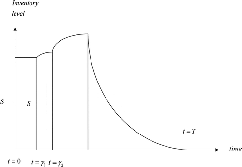
Initially i.e., at time $t=0$, an organization/farm purchase an amount $S$ to start the business. So, at $t=0$, the stock-level is $S$. During the time interval$\left(0,{\gamma }_1\right)$, the stock-level remains unchanged (i.e., there is no amelioration or deterioration) but during the time interval$\left({\gamma }_1,{\gamma }_2\right)$, the stock-level increases due to amelioration effect only. Again, in the time interval$\left({\gamma }_2,t_1\right)$, the stock-level increases due to the effect of amelioration as well as deterioration (as the deterioration rate is much lower than the rate of amelioration) and the stock-level reaches to $S_1$. Then, in the time interval$\left(t_1,T\right)$, the stock-level decreases due to satisfy the demand of the customer’s and the effect of deterioration. Ultimately, the stock-level reaches to zero at time $t=T$. The inventory situation is shown in Figure 1.

Figure 1. The pictorial representation of the proposed inventory system.

The inventory system satisfies the following differential equations:

(1) $q^{\prime }(t)=0;0\le t<{\gamma }_1$(1)

(2) $q^{\prime }(t)=A_1(t)q(t);{\gamma }_1\le t<{\gamma }_2$(2)

(3) $q^{\prime }(t)+\theta (t)q(t)=A_1(t)q(t);{\gamma }_2<t\le t_1$(3)

(4) $q^{\prime }(t)+\theta (t)q(t)=A_1(t)q(t)-D(A,p);t_1<t\le T$(4)

with the conditions

(5a) $q(t)=S\mathrm{a}\mathrm{t}t=0,{\gamma }_1$(5a)

(5b) $q(t)=S_1\mathrm{a}\mathrm{t}t=t_1$(5b)

(5c) $q(t)=0att=T$(5c)

where $A_1(t)={\alpha }_1{\beta }_1(t-{\gamma }_1{)}^{{\beta }_1-1}$ and $\theta (t)={\alpha }_2{\beta }_2(t-{\gamma }_2{)}^{{\beta }_2-1}$

Furthermore, q(t) is continuous at $t={\gamma }_1$, ${\gamma }_2$ and $t_1$.

The solutions of equations (1)–(4) with the conditions (5a)–(5c), we have,

(6) $q(t)=S,0\le t<{\gamma }_1$(6)

(7) $=Sexp\{{\alpha }_1(t-{\gamma }_1{)}^{{\beta }_1}\},{\gamma }_1\le t<{\gamma }_2$(7)

(8) $=S_{1}exp\left[{\alpha }_1\left\{{(t-{\gamma }_1)}^{{\beta }_1}-{\left(t_1-{\gamma }_1\right)}^{{\beta }_1}\right\}-{\alpha }_2\left\{{\left(t-{\gamma }_2\right)}^{{\beta }_2}-{\left(t_1-{\gamma }_2\right)}^{{\beta }_2}\right\}\right],{\gamma }_2<t\le t_1$(8)

(9) $\begin{array}{rl}& =D(A,p)exp\left\{{\alpha }_1{\left(t-{\gamma }_1\right)}^{{\beta }_1}-{\alpha }_2{\left(t-{\gamma }_2\right)}^{{\beta }_2}\right\}\underset{t}{\overset{T}{\int }}exp\left\{{\alpha }_2{\left(t-{\gamma }_2\right)}^{{\beta }_2}-{\alpha }_1{\left(t-{\gamma }_1\right)}^{{\beta }_1}\right\}dt,\\ & t_1<t\le T\end{array}$(9)

Using the continuity of $q(t)$ at $t=t_1,$ we have (from equations (8) and (9)),

(10) $S_1=D(A,p)exp\left\{{\alpha }_1{\left(t_1-{\gamma }_1\right)}^{{\beta }_1}-{\alpha }_2{\left(t_1-{\gamma }_2\right)}^{{\beta }_2}\right\}\underset{t_1}{\overset{T}{\int }}exp\left\{{\alpha }_2{\left(t-{\gamma }_2\right)}^{{\beta }_2}-{\alpha }_1{\left(t-{\gamma }_1\right)}^{{\beta }_1}\right\}dt$(10)

Again $q(t)$ is continuous at $t={\gamma }_2.$ Then from equations (7) and (8), we have,

$Sexp{\alpha }_1({\gamma }_2-{\gamma }_1{)}^{{\beta }_1}$$=S_{1}exp\left[{\alpha }_1\left\{{({\gamma }_2-{\gamma }_1)}^{{\beta }_1}-{\left(t_1-{\gamma }_1\right)}^{{\beta }_1}\right\}-{\alpha }_2\left\{-{\left(t_1-{\gamma }_2\right)}^{{\beta }_2}\right\}\right]$

which implies

(11) $S=S_{1}exp\left[{\alpha }_2{\left(t_1-{\gamma }_2\right)}^{{\beta }_2}-{\alpha }_1{\left(t_1-{\gamma }_1\right)}^{{\beta }_1}\right]$(11)

The total units ameliorated over the cycle is given by

(12) $A^{\prime }=\underset{{\gamma }_1}{\overset{{\gamma }_2}{\int }}{\alpha }_1{\beta }_1{\left(t-{\gamma }_1\right)}^{{\beta }_1-1}q\left(t\right)dt+\underset{{\gamma }_2}{\overset{t_1}{\int }}{\alpha }_1{\beta }_1{\left(t-{\gamma }_1\right)}^{{\beta }_1-1}q\left(t\right)dt+\underset{t_1}{\overset{T}{\int }}{\alpha }_1{\beta }_1{\left(t-{\gamma }_1\right)}^{{\beta }_1-1}q\left(t\right)dt$(12)

The total number of deteriorated units during $\left[{\gamma }_2,T\right]$ is given by

(13) $\begin{array}{rl}& D^{\prime }=\underset{{\gamma }_2}{\overset{t_1}{\int }}\theta \left(t\right)q\left(t\right)dt+\underset{t_1}{\overset{T}{\int }}\theta \left(t\right)q\left(t\right)dt=S_1\underset{{\gamma }_2}{\overset{t_1}{\int }}{\alpha }_2{\beta }_2{(t-{\gamma }_2)}^{{\beta }_2-1}exp\left[{\alpha }_1\left\{{\left(t-{\gamma }_1\right)}^{\beta 1}-{\left(t_1-{\gamma }_1\right)}^{{\beta }_1}\right\}\right.\\ & \left.-\left\{{\alpha }_2\left\{{\left(t-{\gamma }_2\right)}^{{\beta }_2}-{\left(t_1-{\gamma }_2\right)}^{\beta 2}\right\}\right\}\right]dt+\left[\underset{t_1}{\overset{T}{\int }}{\alpha }_2{\beta }_2{(t-{\gamma }_2)}^{{\beta }_2-1}D(A,p)exp\left\{{\alpha }_1{\left(t-{\gamma }_1\right)}^{\beta 1}-{\alpha }_2{\left(t-{\gamma }_2\right)}^{{\beta }_2}\right\}\right.\\ & \left.\left[\underset{t}{\overset{T}{\int }}exp\left\{{\alpha }_2{\left(t-{\gamma }_2\right)}^{{\beta }_2}-{\alpha }_1{\left(t-{\gamma }_1\right)}^{\beta 1}\right\}dt\right]\right]dt\end{array}$(13)

Thus, the salvage value for the entire cycle T is $p^{\prime }{D}^{\prime }.$

Since the demands are fulfilled during$\left[t_1,T\right]$, we have

$S+A^{\prime }-D^{\prime }=D(A,p)(T-t_1)$

which implies

(14) $A^{\prime }=D(A,p)(T-t_1)-S+D^{\prime }$(14)

Thus the total ameliorating cost $=C_a{A}^{\prime }$

Ordering cost $=C_0$ per replenishment

Now the holding cost for the system is $C_{h}S{\gamma }_1+C_{h}H$

(15) $whereH=\left[\underset{{\gamma }_1}{\overset{{\gamma }_2}{\int }}q(t)dt+\underset{{\gamma }_2}{\overset{t_1}{\int }}q(t)dt+\underset{t_1}{\overset{T}{\int }}q(t)dt\right]$(15)

Total advertisement cost of the system is given by

$A_{dc}=G.A$

3.1. System cost and profit function

The total inventory system cost is denoted by $TC$ and is given by

$TC=C_0+C_{p}S+C_{h}H+C_{h}S{\gamma }_1+C_a{A}^{\prime }+A_{dc}$

i.e.,

(16) $TC=C_0+C_{p}S+C_{h}H+C_{h}S{\gamma }_1+C_a\left\{D(A,p)(T-t_1)-S+D^{\prime }\right\}+A_{dc}$(16)

Hence the profit per unit is given by

$Z\left(A,t_1,T\right)=\frac{1}{T}\left[p\underset{t_1}{\overset{T}{\int }}D(A,p)dt+p^{\prime }{D}^{\prime }-TC\right]$

$=\frac{1}{T}\left[pD(A,p)(T-t_1)+p^{\prime }{D}^{\prime }-TC\right]$

Here the profit function $Z(A,t_1,T)$ is a function of three independent variables $A$, $t_1$ and T.

Hence the corresponding nonlinear constrained optimization problem is given by

(16) $MaximizeZ(A,t_1,T)$(16)

subject to ${\gamma }_2<t_1<T\mathrm{a}\mathrm{n}\mathrm{d}A\mathrm{i}\mathrm{s}\mathrm{i}\mathrm{n}\mathrm{t}\mathrm{e}\mathrm{g}\mathrm{e}\mathrm{r}.$

3.2. Special case: when the cycle length t is prescribed

In this case, the corresponding optimization problem can be written as follows:

(17) $Maximize{Z}_1(A,t_1)$(17)

subject to ${\gamma }_2\le t_1<T\mathrm{a}\mathrm{n}\mathrm{d}A\mathrm{i}\mathrm{s}\mathrm{i}\mathrm{n}\mathrm{t}\mathrm{e}\mathrm{g}\mathrm{e}\mathrm{r}.$

where $Z_1(A,t_1)=\frac{1}{T}\left[pD(A,p)(T-t_1)+p^{\prime }{D}^{\prime }-TC\right].$

4. Formulation of mathematical model in interval environment

In this case, model description, differential equations, their solutions and expressions for $S,S_1\mathrm{a}\mathrm{n}\mathrm{d}R\mathrm{w}\mathrm{i}\mathrm{l}\mathrm{l}\mathrm{b}\mathrm{e}\mathrm{t}\mathrm{h}\mathrm{e}\mathrm{s}\mathrm{a}\mathrm{m}\mathrm{e}\mathrm{w}\mathrm{i}\mathrm{t}\mathrm{h}\mathrm{t}\mathrm{h}\mathrm{e}\mathrm{c}\mathrm{r}\mathrm{i}\mathrm{s}\mathrm{p}\mathrm{m}\mathrm{o}\mathrm{d}\mathrm{e}\mathrm{l}\mathrm{d}\mathrm{i}\mathrm{s}\mathrm{c}\mathrm{u}\mathrm{s}\mathrm{s}\mathrm{e}\mathrm{d}\mathrm{e}\mathrm{a}\mathrm{r}\mathrm{l}\mathrm{i}\mathrm{e}\mathrm{r}.$

The salvage value for the entire cycle T is $\left[{p^{\prime }}_L,{p^{\prime }}_U\right]D^{\prime }.$

Here the total ameliorating cost $=C_a{A}^{\prime }=\left[C_{aL},C_{aU}\right]A^{\prime }$

Ordering cost $C_0=\left[C_{0L},C_{0U}\right]$ per replenishment

Now the lower and upper bounds of the holding cost for the system are $C_{hL}S{\gamma }_1+C_{hL}H$and $C_{hU}S{\gamma }_1+C_{hU}H,$

where $H=\left[\underset{{\gamma }_1}{\overset{{\gamma }_2}{\int }}q(t)dt+\underset{{\gamma }_2}{\overset{t_1}{\int }}q(t)dt+\underset{t_1}{\overset{T}{\int }}q(t)dt\right]$Total advertisement cost of the system is given by

$A_{dc}=G.A$

4.1. System cost and profit function

The total system cost $TC$ can be obtained by adding ordering cost, purchase cost, inventory holding cost, shortage cost, ameliorating cost, advertisement cost and lost sale cost.

Thus the upper bound of the total system cost

$T{C}_U=C_{0U}+C_{pU}S+C_{hU}H+C_{hU}S{\gamma }_1+C_{aU}{A}^{\prime }+A_{dc}$

$\mathrm{i}.\mathrm{e}.T{C}_U=C_{0U}+C_{pU}S+C_{hU}H+C_{hU}S{\gamma }_1+C_{aU}\left\{D(A,p)(T-t_1)-S+D^{\prime }\right\}+A_{dc}$

and the lower bound of the total system cost

$T{C}_L=C_{0L}+C_{pL}S+C_{hL}H+C_{hL}S{\gamma }_1+C_{aL}{A}^{\prime }+A_{dc}$

$\mathrm{i}.\mathrm{e}.T{C}_L=C_{0L}+C_{pL}S+C_{hL}H+C_{hL}S{\gamma }_1+C_{aL}\left\{D(A,p)(T-t_1)-S+D^{\prime }\right\}+A_{dc}$

In this case, the profit function (average profit) $Z$ is an interval valued function of the two continuous variables $t_1,\mathrm{T}$ and one integer variable $A.$

Thus the average profit of the system is given by $\left[Z_L(A,t_1,T),Z_U(A,t_1,T)\right]$

$\mathrm{w}\mathrm{h}\mathrm{e}\mathrm{r}\mathrm{e}{Z}_L\left(A,t_1,T\right)=\frac{1}{T}\left[p_L\underset{t_1}{\overset{T}{\int }}D(A,p)dt+{p^{\prime }}_L{D}^{\prime }-T{C}_U\right]=\frac{1}{T}\left[p_{L}D(A,p)(T-t_1)+{p^{\prime }}_L{D}^{\prime }-T{C}_U\right]$

$\mathrm{a}\mathrm{n}\mathrm{d}{Z}_U\left(A,t_1,T\right)=\frac{1}{T}\left[p_{U}D(A,p)(T-t_1)+{p^{\prime }}_U{D}^{\prime }-T{C}_L\right].$

Hence the corresponding optimization problem is given by

(18) $\mathrm{M}\mathrm{a}\mathrm{x}\mathrm{i}\mathrm{m}\mathrm{i}\mathrm{z}\mathrm{e}\left[Z_L(A,t_1,T),Z_U(A,t_1,T)\right]$(18)

subject to ${\gamma }_2<t_1<T\mathrm{a}\mathrm{n}\mathrm{d}A\mathrm{i}\mathrm{s}\mathrm{i}\mathrm{n}\mathrm{t}\mathrm{e}\mathrm{g}\mathrm{e}\mathrm{r}.$

5. Solution procedure

In this section, we have discussed the solution procedure of maximization problems (16), (17) and (18). Clearly, the problems (16) and (17) are highly non-linear deterministic optimization problems. However, the problem (18) is interval valued. Therefore these problems cannot be solved by existing direct/indirect method for getting global optimal solution. To overcome this difficulty, we have solved the above problem by three variants of QPSO techniques. The detailed of these techniques have been discussed in Appendix. Also, for the interval optimization problem, we have used different variants of QPSO, interval arithmetic and interval order relations which have been discussed in Bhunia et al. [29].

6. Numerical Example

6.1. Crisp environment

To illustrate and validate the model numerically, let us consider a hypothetical inventory system of ameliorating item with the following data:

a = 200, b = 0.5, $C_0$= $500/order, $C_p$= $5/unit, $C_h$= $1/unit/unit time, $C_a$= $12/unit, $G$= $50/advertisement, p = $20/unit, $p^{\prime }=$$3/unit, ${\alpha }_1=$0.8, ${\alpha }_2=$0.05, ${\beta }_1=$0.8, ${\beta }_2=$2, ${\gamma }_1=$0.1, ${\gamma }_2=$0.25, $\xi =$0.1

For solving the optimization problem relating to the above hypothetical inventory system, we have used three different variants of QPSO which are coded in C language and the corresponding computation has been performed on a Laptop with i-3, 7 generation 2.40 GHZ processor in Linux environment. In case of each QPSO, 40 independent runs with different sets of random numbers have been performed. The computational results corresponding to the best found value of the average profit obtained techniques of QPSO have been displayed in Table 2. It should be noted that this best found result is either optimal or nearer to optimal solution. However, the theoretical development of optimality cannot be done. Also the statistical analysis corresponding to 40 independent runs has been displayed in Table 3.

Table 2. Computational Results in different techniques of QPSO.

Variants of QPSO	Best found value	t1	T	S	S1	A	Computational time (in Sec.)
GQPSO	1970.7272	0.25	2.2611	214.7396	224.9554	11	0.6329
WQPSO	1970.7272	0.25	2.2601	214.7157	224.9303	11	0.657
AQPSO	1970.7272	0.25	2.2611	214.7397	224.9554	11	0.6323

Table 3. Statistical Analyses for different variants of QPSO.

Variants of QPSO	Best found average profit ($)	Worst found average profit ($)	Mean value of average profit ($)	Standard Deviation of average profit ($)
GQPSO	1970.7272	1970.7272	1970.7272	2.3027 × 10^−13
WQPSO	1970.7272	1970.4463	1970.7083	0.04601104
AQPSO	1970.7272	1970.7272	1970.7272	2.3027 × 10^−13

From the computational results obtained in different variants of QPSO (cf. Table 2) it is observed that the value of $t_1$ coincides with the value of ${\gamma }_2$, the parameter of Weibull distributed deterioration rate. This means that there is no deterioration during the period$\left({\gamma }_2,t_1\right)$. Again from the statistical analyses for different variants of QPSO (cf. Table 3), it is seen that the performances of GQPSO and AQPSO techniques be the same with respect to different characteristics (i.e., Best found, worst found, mean and standard deviation values of average profit). From Table 3, it is seen that Best, Worst found values of average profits and Mean value, Standard deviation values of average profit be the same in case GQPSO and AQPSO methods. However, these are different in WQPSO methods except best found value. So the results obtained from GQPSO and AQPSO be the solution of the numerical example.

6.2. Interval environment

To illustrate and validate the model (in interval environment) numerically, let us consider a hypothetical inventory system of ameliorating item with the following data:

$\mathrm{a}=200,\mathrm{b}=0.4,C_{0L}=\mathrm{\$}490/\mathrm{o}\mathrm{r}\mathrm{d}\mathrm{e}\mathrm{r},C_{0U}=\mathrm{\$}510/\mathrm{o}\mathrm{r}\mathrm{d}\mathrm{e}\mathrm{r},C_{pL}=\mathrm{\$}4/u\mathrm{n}\mathrm{i}\mathrm{t},C_{pU}=\mathrm{\$}6/\mathrm{u}\mathrm{n}\mathrm{i}\mathrm{t},C_{hL}=\mathrm{\$}0.8/\mathrm{u}\mathrm{n}\mathrm{i}\mathrm{t}/\mathrm{u}\mathrm{n}\mathrm{i}\mathrm{t}\mathrm{t}\mathrm{i}\mathrm{m}\mathrm{e},C_{hU}=\mathrm{\$}1.2/\mathrm{u}\mathrm{n}\mathrm{i}\mathrm{t}/\mathrm{u}\mathrm{n}\mathrm{i}\mathrm{t}\mathrm{t}\mathrm{i}\mathrm{m}\mathrm{e},C_{aL}=\mathrm{\$}10/\mathrm{u}\mathrm{n}\mathrm{i}\mathrm{t},C_{aU}=\mathrm{\$}14\mathrm{\$}/\mathrm{u}\mathrm{n}\mathrm{i}\mathrm{t},G_L=\mathrm{\$}48/\mathrm{a}\mathrm{d}\mathrm{v}\mathrm{e}\mathrm{r}\mathrm{t}\mathrm{i}\mathrm{s}\mathrm{e}\mathrm{m}\mathrm{e}\mathrm{n}\mathrm{t},G_U=\mathrm{\$}52/\mathrm{a}\mathrm{d}\mathrm{v}\mathrm{e}\mathrm{r}\mathrm{t}\mathrm{i}\mathrm{s}\mathrm{e}\mathrm{m}\mathrm{e}\mathrm{n}\mathrm{t},\mathrm{p}=\mathrm{\$}20/\mathrm{u}\mathrm{n}\mathrm{i}\mathrm{t},p_L^{\prime }=\mathrm{\$}3/\mathrm{u}\mathrm{n}\mathrm{i}\mathrm{t},p_U^{\prime }=\mathrm{\$}6/\mathrm{u}\mathrm{n}\mathrm{i}\mathrm{t},{\alpha }_1=0.8,{\alpha }_2=0.05,{\beta }_1=0.8,{\beta }_2=2,{\gamma }_1=0.1,{\gamma }_2=0.25,\xi =0.1$

For solving the optimization problem relating to the above hypothetical inventory system, we have used three different variants of QPSO which are coded in C language and the corresponding computation has been performed on a Laptop with i-3, 7 generation 2.40 GHZ processor in Linux environment. In case of each variant of QPSO, 40 independent runs with different random numbers have been performed. The corresponding results of these computations have been shown in Tables 4 and 5.

Table 4. Best found solution for different variants of QPSO.

Variants of QPSO	$Z_L$	$Z_U$	$Z_C$	$Z_R$	t1	T	S	S1	Computational time (in Sec.)
AQPSO	1283.3831	2145.6204	1714.5000	431.1186	0.25	2.3944	236.1301	281.3941	0.2075
GQPSO	1283.6814	2145.3249	1714.5000	430.8217	0.25	2.391	235.9093	281.1309	0.2696
WQPSO	1283.6844	2145.3219	1714.5000	430.8187	0.25	2.391	235.9071	281.1283	0.2667

Table 5. Statistical analyses for different variants of QPSO.

Variants of QPSO	Best found Centre Value of average profit	Worst found Centre Value of average profit	Mean value Centre Value of average profit	Standard Deviation of average profit
AQPSO	1714.5000	1714.5000	1714.5000	0
GQPSO	1714.5000	1714.5000	1714.5000	0
WQPSO	1714.5000	1714.5000	1714.5000	0

From Table 4, it is observed that the Centre value of interval valued average profit be the same for all the variants of QPSO. However the radius of interval valued average profit of WQPSO technique is the largest with respect to other two variants. On the other hand, the computational time for best found solution of AQPSO technique is the lowest than GQPSO and WQPSO.

Again, Table 5 shows that the best found, worst found and mean Centre values of interval valued average profit for all the variants of QPSO be the same. On the other hand the standard deviation values of all the QPSO be zero. This means that for all QPSO, the computational results are stable.

7. Sensitivity analyses

7.1. Crisp environment

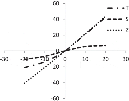
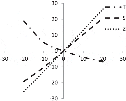
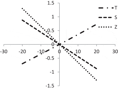
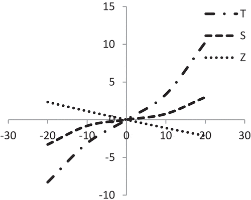
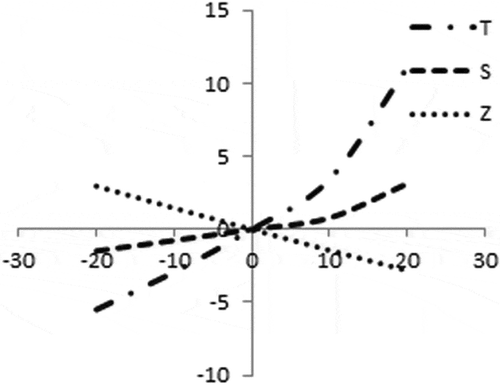
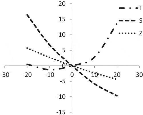
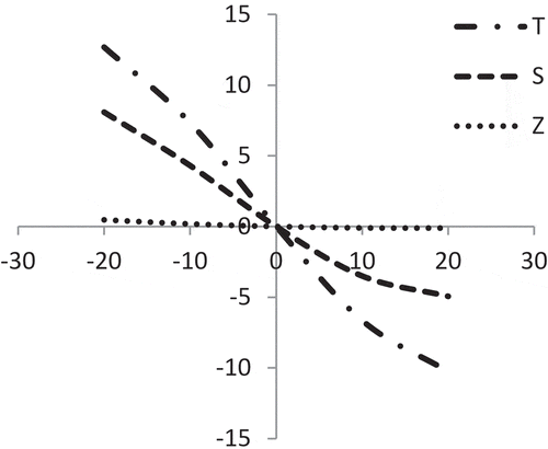
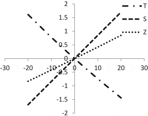
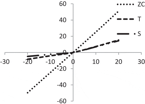
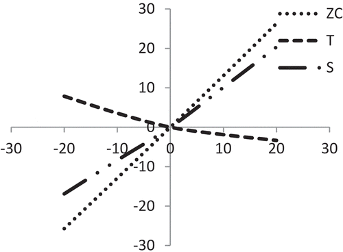
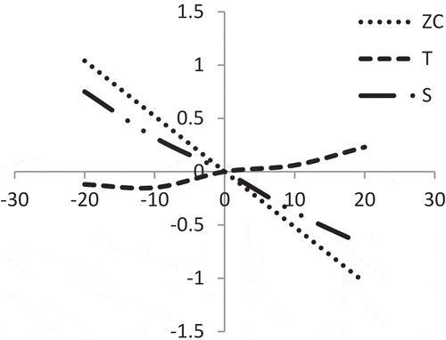
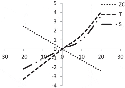
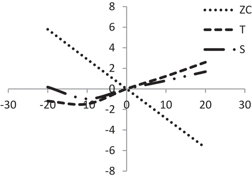
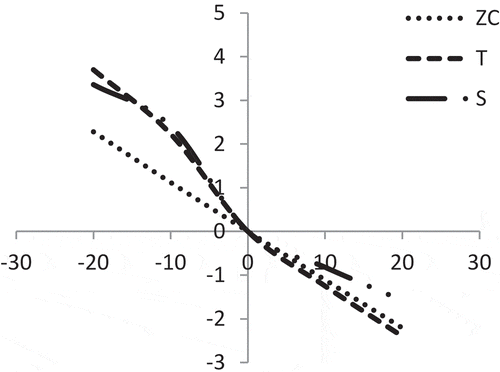
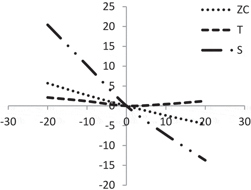
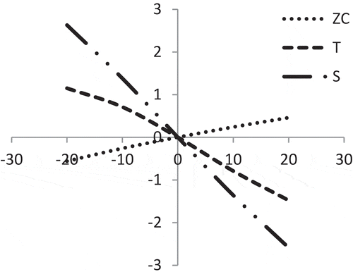
To investigate the impact of different system parameters on the cycle length (T), initial stock level (S) and the average profit (Z), sensitivity analyses have been performed geometrically considering the earlier mentioned numerical example. This experiment has been performed by GQPSO. The results have been obtained by changing one system parameter at a time and keeping the other parameters at their original values. In each case, the best found results have been taken among 40 runs. The computational results of these analyses have been shown graphically in Figs. 2–9.

Figure 2. Effect of percentage changes of ‘p’ on T, S and Z.

Figure 3. Effect of percentage changes of ‘a’ on T, S and Z.

Figure 4. Effect of percentage changes of ‘b’ on T, S and Z.

Figure 5. Effect of percentage changes of ‘C₀’on T, S and Z.

Figure 6. Effect of percentage changes of ‘Cp’ on T, S and Z.

Figure 7. Effect of percentage changes of ‘α₁’ on T, S and Z.

Figure 8. Effect of percentage changes of ‘β₁’on T, S and Z.

Figure 9. Effect of percentage changes of ‘γ₁’on T, S and Z.

Figure 2 represents that the average profit (Z) is highly sensitive with the changes of selling price (p) whereas the cycle length ($T$) and initial stock-level ($S$) are moderately sensitive for positive or negative changes of ‘p’.

Figure 3 shows that the average profit (Z) and initial stock-level (S) are mostly equally sensitive with the changes of location parameter ‘a’ of demand. On the other hand, the cycle length (T) is less sensitive but it has reverse effect.

It is evident from Figure 4 that with respect to shape parameter ‘b’ of demand, all Z, S and T are less sensitive but reverse effect except T.

In Figure 5, it is observed that all Z, S and T are moderately sensitive with respect to the ordering cost. However, the value of Z has the reverse impact.

Figure 6 presents that the value of T is moderately sensitive but reverse for the changes of the purchase cost. However, the values of S and Z are less sensitive.

From Figure 7, it is seen that the location parameter ‘α₁’ of amelioration rate has negative impact on Z and S. It is also observed that S is equally sensitive; Z is less sensitive with respect to ‘α₁’. On the other hand, when ‘α₁’ decreases, T is insensitive and for increasing ‘α₁’ it is quite equally sensitive.

Figure 8 shows that the shape parameter ‘${\beta }_1$’ of amelioration has the reverse effect on S, T and Z. In cases of S and T, effects are less whereas in cases of Z effect is negligible.

Figure 9 also represents that the average profit ($Z$), the cycle length ($T$) and initial stock-level ($S$) are less sensitive with the changes of ‘${\gamma }_1$’but T has the reverse effect.

7.2 Interval environment

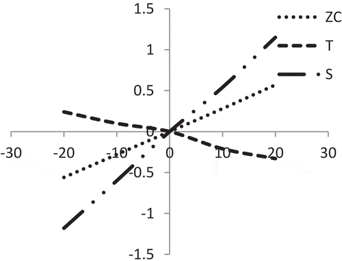
To investigate the impact of different system parameters on the cycle length (T), initial stock level (S) and the average profit (Z_C), sensitivity analyses have been performed geometrically considering the earlier mentioned numerical example. This experiment has been performed by AQPSO. The results have been obtained by changing one system parameter at a time and keeping the other parameters at their original values. In each case, the best found results have been taken among 40 runs. The results of these analyses have been shown graphically in Figs. 10–18.

Figure 10. Effect of percentage changes of ‘p’ on T, S and Z_C.

Figure 11. Effect of percentage changes of ‘a’ on T, S and Z_C.

Figure 12. Effect of percentage changes of ‘b’ on T, S and Z_C.

Figure 13. Effect of percentage changes of ‘C_o’on T, S and Z_C.

Figure 14. Effect of percentage changes of ‘C_p’on T, S and Z_C.

Figure 15. Effect of percentage changes of ‘C_h’ on T, S and Z_C.

Figure 16. Effect of percentage changes of ‘α₁’ on T, S and Z_C.

Figure 17. Effect of percentage changes of ‘β₁’ on T, S and Z_C.

Figure 18. Effect of percentage changes of ‘γ₁’ on T, S and Z_C.

Figure 10 represents the average profit (Z_C) is highly sensitive with the changes of selling price (p) whereas the cycle length ($T$) and initial stock-level ($S$) are moderately sensitive for positive or negative changes of ‘p’.

Figure 11 shows that the average profit (Z_C) and initial stock-level (S) are mostly equally sensitive with the changes of the location parameter ‘a’ of demand. On the other hand, the cycle length (T) is less sensitive but it has reverse effect.

It is evident from Figure 12 that with respect to the shape parameter ‘b’ of demand, all Z_C, S and T are less sensitive but reverse effect except T.

In Figure 13, it is observed that all Z_C, S and T are less sensitive with respect to lower and upper bounds of ordering cost respectively. However, the value of Z_C has reverse impact.

Figure 14 presents that the values of Z_C is moderately sensitive but reverse effect for the change of the purchase cost. However, the values of S and T are less sensitive.

In Figure 15, it is observed that all Z_C, S and T are less sensitive with respect to the lower and upper bound of holding cost, respectively.

From Figure 16, it is seen that the location parameter ‘α₁’ of amelioration has negative impact on Z_C and S. It is also observed that S is equally sensitive, Z_C is less sensitive, T is insensitive.

Figure 17 shows that the shape parameter ‘${\beta }_1$’ of amelioration has reverse effect on S and T. In cases of S and T, effects are less whereas in cases of Z_C effect is negligible.

Figure 18 also represents that the average profit (Z_C), the cycle length ($T$) and initial stock-level ($S$) are less sensitive with the changes of ‘${\gamma }_1$’but T has the reverse.

8. Concluding remarks

In this work, two inventory models have been developed for ameliorating item considering variable demand dependent on frequency of advertisement and selling price of the item under crisp and interval environments. The main contribution of this work is to consider both the amelioration and deterioration effects of the ameliorating item and imprecise (interval uncertainty) inventory costs of the items. Here, it is assumed that the effect of amelioration starts after certain time and its rate increases continuously with the rate which follows three-parameter Weibull distribution. Also, at the same time, Weibull distributed deterioration has been considered. The cost for feeding the ameliorating items has been taken into account. Due to three-parameter Weibull distribution of both amelioration and deterioration, the corresponding optimization problem is converted to highly nonlinear in nature and also interval valued. So, it is a formidable task to solve both problems by any gradient based method/direct method. To avoid this complication, three different variants of QPSO technique have been used for solving the optimization problems. Finally, sensitivity analyses have been studied graphically for each model in order to investigate the effects of changes of different system parameters on optimal policy.

This work can further be enhanced in different ways. One such way is to consider trade credit (single level, two levels or three levels) policy in the proposed inventory model. Anyone can extend these models by considering the price and stock dependent demand, time dependent demand, non-linear holding cost, inflation etc. On the other hand, this problem can be extended by considering the inventory parameters as interval valued or fuzzy valued.

The present model is useful for life stocks. Its importance has been seen in the developing countries like India, Bangladesh, Pakistan, Nepal, etc. as the culture of life stocks like fast growing animals has been taken up now-a-days in a very large scale.

Acknowledgments

The first author greatly acknowledge the financial support given by CSIR (New Delhi) under CSIR-JRF Fellowship (Award No. 09/025(0246)/2019-EMR-I). Also, the authors are grateful to all the anonymous reviewers for their constructive suggestions to modification of the paper.

Disclosure statement

No potential conflict of interest was reported by the authors.

Additional information

Funding

This work was supported by the Rajan Mondal CSIR-JRF [Award No. 09/025(0246)/2019-EMR-I].

Appendix

Particle Swarm Optimization

Quantum behaved particle swarm optimization (QPSO) is an efficient technique based on the quantum behaviour of the particle. Sun et al. [30] first proposed this algorithm considering quantum behaviour of the particle. As the mean-optimal position (MP) enhances the cooperation between particles and particles’ waiting with each other, QPSO can prevent particles trapping into local minima (Pan et al. [31]). However, the speed and accuracy of convergence algorithm are also slow. In QPSO, the $k-\mathrm{t}\mathrm{h}$ component of the position of $j-\mathrm{t}\mathrm{h}$ particle is given by

$x_{jk}^{(i+1)}={\tilde{p}}_{jk}^{(i)}\pm {\beta }^{\prime }\left|m_k^{(i)}-x_{jk}^{(i)}\right|log\left(\frac{1}{u_k}\right),\mathrm{w}\mathrm{h}\mathrm{e}\mathrm{r}\mathrm{e}j=1,2,...,p\mathrm{\_}size\mathrm{a}\mathrm{n}\mathrm{d}k=1,2,...,n$

where $u_k$ is a uniformly distributed random number in (0, 1), ${\beta }^{\prime }$, the coefficient of contraction-expansion used to control the convergence speed of the algorithm. Its value decreases linearly from 1.0 to 0.5. $m_k^{(i)}$ is the $k-\mathrm{t}\mathrm{h}$ component of $m^{(i)}$, the mean of the personal best (pbest) position of all the particles of the population at $i-\mathrm{t}\mathrm{h}$ iteration. ${\tilde{p}}_{jk}$ be the $k-\mathrm{t}\mathrm{h}$ component of local attractor ${\tilde{p}}_j$ of $j-\mathrm{t}\mathrm{h}$ particle. The different component of local attractor ${\tilde{p}}_j$ of $j-\mathrm{t}\mathrm{h}$ particle is given by

${\tilde{p}}_{jk}^{(i)}=\left[{\tau }_1{r}_{1k}^{(i)}p{b}_{jk}^{(i)}+{\tau }_2{r}_{2k}^{(i)}{p}_{gk}^{(i)}\right]/\left({\tau }_1{r}_{1k}^{(i)}+{\tau }_2{r}_{2k}^{(i)}\right),k=1,2,...,n$

$\mathrm{O}\mathrm{r},{\tilde{p}}_{jk}^{(i)}={\psi }_{k}p{b}_{jk}^{(i)}+(1-{\psi }_k)p_{gk}^{(i)},k=1,2,...,n$

where ${\psi }_k=\frac{{\tau }_1{r}_{1k}^{(i)}}{{\tau }_1{r}_{1k}^{(i)}+{\tau }_2{r}_{2k}^{(i)}},k=1,2,...,n$

$\mathrm{i}.\mathrm{e}.,{\psi }_k\in U(0,1)$

Here for maximization of $f$, particle’s pbest position is given by

$p{b}_i^{(0)}=x_i^{(0)}$

$p{b}_i^{(k+1)}=\left\{\begin{array}{c}p{b}_i^{(k)}iff(p{b}_i^{(k)})\ge f(x_i^{(k+1)})\\ x_i^{(k+1)}iff(p{b}_i^{(k)})<f(x_i^{(k+1)})\end{array}\right.$

The global best (gbest) position $p_g$ at (k + 1) -th iteration is given by

$p_g^{(k+1)}=arg\underset{p{b}_i}{max}f(p{b}_i^{(k+1)}),1\le i\le p\mathrm{\_}size$

Again $m^{(k)}=\left(m_1,m_2,...,m_n^{(k)}\right)$

$=\left(\frac{1}{p\mathrm{\_}size}\sum _{i=1}^{p\mathrm{\_}size}{p}_{i1}^{(k)},\frac{1}{p\mathrm{\_}size}\sum _{i=1}^{p\mathrm{\_}size}{p}_{i2}^{(k)},\dots ,\frac{1}{p\mathrm{\_}size}\sum _{i=1}^{p\mathrm{\_}size}{p}_{in}^{(k)}\right)$

After development of QPSO, several researchers proposed different enhanced variants of QPSO. In this context, the enhanced variants WQPSO (Xi et al. [32]), GQPSO (Santos and Coelho [33]), AQPSO (Sun et al. [34]), RQPSO, RRQPSO, SRQPSO (Pan et al. [31]) are worth mentioning. Recently, Bhunia and Shaikh [35] applied WQPSO and GQPSO for solving deteriorated inventory model with two storage facilities under trade credit financing. The details about WQPSO and GQPSO are available in Bhunia and Shaikh [35]. Here we have discussed about AQPSO only.

Adaptive Quantum-Behaved Particle Swarm Optimization (AQPSO)

This technique is dependent on attraction and repulsion phases distinguished by the creativity parameter $\tilde{\beta }$ defined as follows:

1. Attraction phase: $\tilde{\beta }={\tilde{\beta }}_a$when ${\tilde{\beta }}_a\le 1$

2. Repulsion phase: $\tilde{\beta }={\tilde{\beta }}_r$ when ${\tilde{\beta }}_r>1$

When $\tilde{\beta }={\tilde{\beta }}_a$, the particle is bounded to converge to its local attracter $\tilde{p}$ and consequently the diversity decreases. When diversity <$d_{low}$, the system switches over to the repulsion phase ($\tilde{\beta }={\tilde{\beta }}_r$) and some of the particles will depart from $\tilde{p}$.

Again, when the diversity reaches a higher bound ($d_{high}$), then the system will over to the attraction phase again. As a result, this algorithm is based on the diversity of the swarm measured by

diversity $(d)=\frac{1}{\left|p_{size}\right|\left|L\right|}\sum _{j=1}^{\left|p_{size}\right|}\sqrt{\sum _{k=1}^n{({\tilde{p}}_{jk}-m^{(i)})}^2}$

where $\left|L\right|$ is the length of the longest diagonal in the search space.

Again, ${\tilde{p}}_{ij}^{(k)}$and $m^{(k)}$are calculated as follows:

${\tilde{p}}_{ij}^{(k)}={\psi }_j{p}_{ij}^{(k)}+(1-{\psi }_j)p_{gj}^{(k)},j=1,2,\dots ,n$

$\begin{array}{rl}& m^{(k)}=\left(m_1^{(k)},m_2^{(k)},...,m_n^{(k)}\right)\\ & =\left(\frac{1}{p_{size}}\sum _{i=1}^{p_{size}}{\tilde{p}}_{i1}^{(k)},\frac{1}{p_{size}}\sum _{i=1}^{p_{size}}{\tilde{p}}_{i2}^{(k)},...,\frac{1}{p_{size}}\sum _{i=1}^{p_{size}}{\tilde{p}}_{in}^{(k)}\right)\end{array}$

Hence the iterative equation of the particle is given by

$x_{ij}^{(k+1)}={\tilde{p}}_{ij}^{(k)}\pm \tilde{\beta }\left|m_j^{(k)}-x_{ij}^{(k)}\right|log\left(\frac{1}{u_{ij}^{(k)}}\right)$

where $\tilde{\beta }$ decrease linearly from $d_{high}(>1)$to $d_{low}(<1),$$u_{ij}^{(k)}$be a random number uniformly distributed in (0,1).

AQPSO Algorithm

1. Assign the lower and upper bounds of decision variables and different parameters of AQPSO.

2. Initialize a population of particles.

3. Compute the fitness of population.

4. Do the following until the termination criterion is satisfied:

(a) Calculate the mean best (mbest) position.

(b) Measure the diversity (d) of the swarm.

(c) If $d<d_{low},$ assign $\tilde{\beta }={\tilde{\beta }}_a$.

(d) If $d>d_{high},$ assign $\tilde{\beta }={\tilde{\beta }}_r$.

(e) Update the position of each particle.

(f) Store better one as pbest by comparing each particle’s position with the particle’s pbest position according to their fitness value.

(g) Store better one as gbest by comparing current gbest position with earlier gbest position according to their fitness value.

(v) Print the fitness of global best particle with its position.

(vi) End.

References

- H.S. Hwang, A study on an inventory model for items with Weibull ameliorating, Comp. Ind. Eng. 33 (3–4) (1997), pp. 701–704. doi:10.1016/S0360-8352(97)00226-X.
- B. Mondal, A.K. Bhunia, and M. Maiti, An inventory system of ameliorating items for price dependent demand rate, Comput. Ind. Eng. 45 (3) (2003), pp. 443–456. doi:10.1016/S0360-8352(03)00030-5.
- I. Moon, B.C. Giri, and B. Ko, Economic order quantity models for ameliorating/deteriorating items under inflation and time discounting, Eur. J. Oper. Res. 162 (3) (2005), pp. 773–785. doi:10.1016/j.ejor.2003.09.025.
- G.C. Mahata and S.K. De, An EOQ inventory system of ameliorating items for price dependent demand rate under retailer partial trade credit policy, Opsearch 53 (4) (2016), pp. 889–916. doi:10.1007/s12597-016-0252-y.
- Vandana and H.M. Srivastava, An inventory model for ameliorating/deteriorating items with trapezoidal demand and complete backlogging under inflation and time discounting, Math. Methods Appl. Sci. 40 (8) (2017), pp. 2980–2993. doi:10.1002/mma.4214.
- A.A. Taleizadeh, M. Noori-daryan, and L.E. Cárdenas-Barrón, Joint optimization of price, replenishment frequency, replenishment cycle and production rate in vendor managed inventory system with deteriorating items, Int. J. Prod. Econ. 159 (2015), pp. 285–295. doi:10.1016/j.ijpe.2014.09.009.
- N.H. Shah and L.E. Cárdenas-Barrón, Retailer’s decision for ordering and credit policies for deteriorating items when a supplier offers order-linked credit period or cash discount, Appl. Math. Comput. 259 (2015), pp. 569–578. doi:10.1016/j.amc.2015.03.010.
- S. Tiwari, L.E. Cárdenas-Barrón, A. Khanna, and C.K. Jaggi, Impact of trade credit and inflation on retailer’s ordering policies for non-instantaneous deteriorating items in a two-warehouse environment, Int. J. Prod. Econ. 176 (2016), pp. 154–169. doi:10.1016/j.ijpe.2016.03.016.
- A.A. Shaikh, A two warehouse inventory model for deteriorating items with variable demand under alternative trade credit policy, Int. J. Logist. Syst. Manage. 27 (1) (2017), pp. 40–61. doi:10.1504/IJLSM.2017.083221.
- A.K. Bhunia and A.A. Shaikh, Investigation of two-warehouse inventory problems in interval environment under inflation via particle swarm Optimization, Math. Comp. Model. Dyn. Syst. 22 (2) (2016), pp. 160–179. doi:10.1080/13873954.2016.1150860.
- C.K. Jaggi, L.E. Cárdenas-Barrón, S. Tiwari, and A. Shafi, Two-warehouse inventory model for deteriorating items with imperfect quality under the conditions of permissible delay in payments, ScientiaIranica Transac. E 24 (2017), pp. 390–412.
- A.A. Shaikh, L.E. Cardenas-Barron, and S. Tiwari, A two-warehouse inventory model for non-instantaneous deteriorating items with interval valued inventory costs and stock dependent demand under inflationary conditions, Neural Comput. App. 31 (6) (2019), pp. 1931–1948.
- S. Tiwari, C.K. Jaggi, M. Gupta, and L.E. Cárdenas-Barrón, Optimal pricing and lot-sizing policy for supply chain system with deteriorating items under limited storage capacity, Int. J. Prod. Econ. 200 (2018), pp. 278–290. doi:10.1016/j.ijpe.2018.03.019.
- T.P. Hsieh and C.Y. Dye, Optimal dynamic pricing for deteriorating items with reference price effects when inventories stimulate demand, Eur. J. Oper. Res. 262 (1) (2017), pp. 136–150. doi:10.1016/j.ejor.2017.03.038.
- S. Tiwari, L.E. Cárdenas-Barrón, M. Goh, and A.A. Shaikh, Joint pricing and inventory model for deteriorating items with expiration dates and partial backlogging under two-level partial trade credits in supply chain, Int. J. Prod. Econ. 200 (2018), pp. 16–36. doi:10.1016/j.ijpe.2018.03.006.
- S.S. Sunni and W.I.E. Chukwu, An economic order quantity model for items with three-parameter Weibull distribution deterioration, ramp-type demand and shortages, Appl. Math. Model. 37 (23) (2013), pp. 9698–9706. doi:10.1016/j.apm.2013.05.017.
- A. K. Bhunia and A. A. Shaikh, A deterministic inventory model for deteriorating items with selling price dependent demand and three-parameter Weibull distributed deterioration, Int. J. Ind. Eng. Comput. 5 (3) (2014), pp. 497–510. doi:10.5267/j.ijiec.2014.2.002.
- S.S. Sunni and W.I. Chukwu, An inventory model with three-parameter Weibull deterioration, quadratic demand rate and shortages, Am. J. Math. Manage. Sci. 35 (2) (2016), pp. 159–170. doi:10.1080/01966324.2015.1126697.
- D. Chakraborty, D.K. Jana, and T.K. Roy, Two-warehouse Partial Backlogging Inventory Model with Ramp Type Demand Rate, Three-parameter Weibull Distribution Deterioration under Inflation and Permissible Delay in Payments, Comp. & Ind. Eng. 123 (2018), pp.157–179. doi:10.1016/j.cie.2018.06.022.
- S. Tiwari, L.E. Cárdenas-Barrón, A.A. Shaikh, and M. Goh, Retailer’s optimal ordering policy for deteriorating items under order-size dependent trade credit and complete backlogging, Comp. & Ind. Eng. (2018) doi:10.1016/j.cie.2018.12.006 (Online).
- L.E. Cárdenas-Barrón, A.A. Shaikh, S. Tiwari, and G. Treviño-Garza, An EOQ inventory model with nonlinear stock dependent holding cost, nonlinear stock dependent demand and trade credit, Comp. & Ind. Eng. (2018) doi:10.1016/j.cie.2018.12.004.
- R.K. Gupta, A.K. Bhunia, and S.K. Goyal, An application of genetic algorithm in a marketing oriented inventory model with interval valued inventory costs and three-component demand rate dependent on displayed stock level, Appl. Math. Comput. 192 (2) (2007), pp. 466–478. doi:10.1016/j.amc.2007.03.022.
- A.K. Bhunia and A.A. Shaikh, Investigation of two-warehouse inventory problems in interval environment under inflation via particle swarm optimization, Math. Comp. Model. Dyn. Syst. 22 (2) (2016), pp. 160–179. doi:10.1080/13873954.2016.1150860.
- A.A. Shaikh, L.E. Cárdenas-Barrón, and S. Tiwari, A two-warehouse inventory model for non-instantaneous deteriorating items with interval-valued inventory costs and stock-dependent demand under inflationary conditions, Neural Comput. Appl. 31 (6) (2019) pp. 1931–1948.
- A.K. Bhunia, A.A. Shaikh, and L.E. Cárdenas-Barrón, A partially integrated production inventory model with interval valued inventory costs, variable demand and flexible reliability, Appl. Soft. Comput. 55 (2017), pp. 491–502. doi:10.1016/j.asoc.2017.02.012.
- A.A. Shaikh, A.K. Bhunia, L.E. Cárdenas-Barrón, L. Sahoo, and S. Tiwari, A fuzzy inventory model for a deteriorating item with variable demand, permissible delay in payments and partial backlogging with shortage follows inventory (SFI) policy, Int. J. Fuzzy Syst. 20 (5) (2018), pp. 1606–1623. doi:10.1007/s40815-018-0466-7.
- A.A. Shaikh, S.C. Das, A.K. Bhunia, G.C. Panda, and M.A.A. Khan, A two-warehouse EOQ model with interval-valued inventory cost and advance payment for deteriorating item under particle swarm optimization, Soft Comput. (2019), pp. 1–16 (to be appeared).
- J. Sun, B. Feng, and W.B. Xu, Particle swarm optimization with particles having quantum behavior, IEEE Proc. Congr. Evol. Comput. 1 (2004), pp. 325–331.
- D. Pan, Y. Ci, M. He, and H. He, An improved quantum-behaved particle swarm optimization algorithm based on random weight, J, Software 8 (2013), pp. 1327–1332.
- M. Xi, J. Sun, and W. Xu, An improved quantum-behaved particle swarm optimization algorithm with weighted mean best position, Appl. Math. Comput. 205 (2008), pp. 751–759. doi:10.1016/j.amc.2008.05.135.
- D. Santos and L. Coelho, Gaussian quantum-behaved particle swarm optimization approaches for constrained engineering design problems, Expert Syst. Appl. 37 (2) (2010), pp. 1676–1683. doi:10.1016/j.eswa.2009.06.044.
- J. Sun, W.B. Xu, and B. Feng, Adaptive parameter selection of quantum-behaved particle swarm optimization on global level, Adv. Intell. Comput. Lect. Notes Comput. Sci. 3644 (2005), pp. 420–428.
- A.K. Bhunia, A.A. Shaikh, and R.K. Gupta, A study on two warehouse partially backlogged deteriorating inventory models under inflation via particle swarm optimization, Int. J. Syst. Sci. 46 (6) (2015), pp. 1036–1050. doi:10.1080/00207721.2013.807385.
- S.T. Law and H.M. Wee, An integrated production-inventory model for ameliorating and deteriorating items taking account of time discounting, Math. Comput. Model. 43 (5–6) (2006), pp. 673–685. doi:10.1016/j.mcm.2005.12.012.
- H.M. Wee, S.T. Lo, J. Yu, and H.C. Chen, An inventory model for ameliorating and deteriorating items taking account of time value of money and finite planning horizon, Int. J. Syst. Sci. 39 (8) (2008), pp. 801–807. doi:10.1080/00207720801902523.
- S.S. Sana, Demand influenced by enterprises’ initiatives—A multi-item EOQ model of deteriorating and ameliorating items, Math. Comput. Model. 52 (1–2) (2010), pp. 284–302. doi:10.1016/j.mcm.2010.02.045.
- H. Dem and S.R. Singh, A production model for ameliorating items with quality consideration, Int. J. Oper. Res. 17 (2) (2013), pp. 183–198. doi:10.1504/IJOR.2013.053622.