On the combination of kernel principal component analysis and neural networks for process indirect control

ABSTRACT

A new adaptive kernel principal component analysis (KPCA) for non-linear discrete system control is proposed. The proposed approach can be treated as a new proposition for data pre-processing techniques. Indeed, the input vector of neural network controller is pre-processed by the KPCA method. Then, the obtained reduced neural network controller is applied in the indirect adaptive control. The influence of the input data pre-processing on the accuracy of neural network controller results is discussed by using numerical examples of the cases of time-varying parameters of single-input single-output non-linear discrete system and multi-input multi-output system. It is concluded that, using the KPCA method, a significant reduction in the control error and the identification error is obtained. The lowest mean squared error and mean absolute error are shown that the KPCA neural network with the sigmoid kernel function is the best.

KEYWORDS:

• Neural networks
• modelling
• indirect control
• KPCA
• reduction
• non-linear system

1. Introduction

We are involved in adaptive system control of the non-linear discrete system using neural network. In fact, the indirect adaptive control structure is based on two neural network blocks corresponding to the model identification of the dynamic behaviour of the system and system controller [1–6].

However, the size of the neural network model or the neural network controller can accelerate or slow down their training phase. This problem of reduction of the higher dimension of neural network is well discussed by different techniques [7–37].

The first step in reduction method is feature selection (new features are selected from the original inputs) or feature extraction (new features are transformed from the original inputs). In the modelling, all available indicators can be used, but correlated features or irrelevant features could deteriorate the generalization performance of any model [7–18].

Many linear techniques of reduction dimensionality are proposed. For instance, Kohonen Self Organizing Feature Maps provide a way of representing multidimensional data in much lower dimensional spaces [19], curvilinear component analysis[20] and curvilinear distance analysis [21] are proposed to make smaller the original dimension of the face images, data and for classification in medical imaging [22] and principal component analysis (PCA) has been widely used for reducing high dimension in many applications [16–18,23–25].

PCA is a well-known method for feature extraction [23,24]. By calculating the eigenvectors of the covariance matrix of the original inputs, PCA linearly transforms the original high-dimensional input vector into new low-dimensional one whose components are uncorrelated. The basis function orders of PCA, as a typical approach, are the lowest in the sense of model dimension reduction [16–18,23–25].

In other applications, for instance, in the study by Zhang et al. [15], a hybrid modelling strategy consists of a decoupled non-linear radial basis function neural network model based on PCA and linear autoregressive exogenous model. PCA reduces the cross-validation time required to identify optimal model hyper-parameters [25]. In the study by Seerapu and Srinivas [26], it was combined with the linear discriminate analysis to ameliorate the reduction. Then, in the study by Peleato et al. [27], the use of fluorescence data coupled with neural networks based on PCA for improved predictability of drinking water disinfection by-products was investigated. Second, in the study by Qinshu et al. [14], a PCA for feature selection and a grid searching and k-fold cross validation approach for parameter optimization in the support vector machine were developed. Finally, in other dimensionality reduction, linear techniques such as multidimensional scaling and probabilistic PCA are applied for user authentication using keystroke dynamics [28] and other methods [29].

However, PCA is a linear time/space separation method and cannot be directly applied to non-linear systems [30]. Non-linear PCA has also been developed by using different algorithms. Kernel principal component analysis (KPCA) is a non-linear PCA developed by using the kernel method. Kernel method is originally used for Support Vector Machine (SVM). Later, it has been generalized into many algorithms having the term of dot products such as PCA. Specifically, KPCA firstly maps the original inputs into a high-dimensional feature space using the kernel method and then calculates PCA in the high-dimensional feature space. The linear PCA in the high-dimensional feature space corresponds to a non-linear PCA in the original input space. Recently, another linear transformation method called independent component analysis (ICA) is also developed. Instead of transforming uncorrelated components, ICA attempts to achieve statistically independent components in the transformed vectors. ICA is originally developed for blind source separation. Later, it has been generalized for feature extraction [7].

KPCA is used as an effective method for tackling the problem of non-linear data [31]. Indeed, in the study by Chakour et al. [32], an algorithm for adaptive KPCA is proposed for dynamic process monitoring. This algorithm combined two existing algorithms: the recursive weighted PCA and the moving window KPCA algorithms. Even better, the fault detection of the non-linear system using KPCA method for extracting the reduced number of measurements from the training data [33] is studied. In the study by Xiao and He [34], a neural-network-based fault diagnosis approach of analog circuits is developed, using maximal class separability-based KPCA as a preprocessor to reduce the dimensionality of candidate features so as to obtain the optimal features with maximal class separability as inputs to the neural networks. In the study by Reddy and Ravi [36], differential evolution (DE)-trained kernel principal component wavelet neural network and DE-trained kernel binary quantile regression are proposed for classification. In the proposed DE-KPCWNN technique, KPCA is applied to input data to get KPC, on which WNN is employed.

In the study by Klevecka and Lelis [37], a functional algorithm of preprocessing of input data taking into account the specific aspects of teletraffic and properties of neural networks is created. The practical application for forecasting telecommunication data sequences shows that the procedure of data preprocessing decreases the time of learning and increases the plausibility and accuracy of the forecasts.

In this paper, the scheme of indirect adaptive control is used based on a neural network. First, the used neural network is based on an adaptive learning rate and a reduced derivative of the activation function. Even better, the weights of the neural network model and neural network controller are updated based on the identification error and the control error and used to generate the appropriate control.

In the first hand, in various studies [1,2,5,6,15,38,39], the authors developed many algorithms for the adaptive indirect control without any preprocessing and they did not take into account the high dimension of the neural network.

On the other hand, in the study by Errachdi and Benrejeb [4], the authors developed an algorithm to accelerate the speed of training phase in the adaptive indirect control based on neural network controller using a variable learning rate and a development of Taylor of the derivative of the activation function but they did not focus on the big dimension. That is why, in this paper, we propose a new algorithm of a reduction of the input vector of the neural controller in the control system based on the KPCA. The procedure of the data preprocessing scheme decreases the time of learning and increases the accuracy of the system control.

The present paper is organized as follows. After this introduction, Section 2 reviews the proposed KPCA method for system control. In fact, the proposed neural network controller based on the KPCA method is developed. Furthermore, in Section 3, the proposed algorithm is detailed. In Section 4, an example of a non-linear system is presented to illustrate the proposed efficiency of the method. Section 5 gives the conclusion of this paper.

2. The proposed KPCA neural network controller approach

On the basis of the input and output relations of a system, the above discrete non-linear system can be expressed by a NARMA (Non-linear Autoregressive Moving Average) model [4,35] given by (1) $y(k+1)=f(y(k),...,y(k-n_y),u(k),...,u(k-n_u))$(1)

$f(.)$ is the non-linear function mapping specified by the model, $y(k)$ and $u(k)$ are the outputs and the inputs of the system, respectively, $k$ is the discrete time, $n_y$ and $n_u$ are the number of past output and input samples, respectively, required for prediction.

The aim of this paper is to find a control law $u(k)$ to the non-linear system, given by Equation (1), based on the KPCA approach in order that the system output $y(k)$ tracks, where possible, the desired value $r(k)$.

The indirect control architecture is shown in Figure 1, and the weights of the neural network model and the neural network controller are trained by different errors where $e(k)$ is the identification error, ${\hat{e}}_c(k)$ is the estimated tracking error and $e_c(k)$ is the tracking error [4].

Figure 1. The architecture of indirect neural control.

The architecture shown in Figure 1 assumes the role of two neural blocks. Indeed, the weights of the neural model are adjusted by the identification error $e(k)$; however, the weights of the neural controller are trained by the tracking error $e_c(k)$ [4].

The multi-layer perceptron is used in the neural model and in the neural controller. Each block consists of three layers. The sigmoid activation function $s(.)$ is used for all neurons [4].

2.1. The neural network model

The principle of neural network model is given by the Figure 2.

Figure 2. The principle of neural network model.

The ${\mathrm{j}}^{\mathrm{t}\mathrm{h}}$ output layer of the hidden layer is described as follows: (2) $h_j=\sum _{i=1}^{n_1}{w}_{ji}{x}_{i}j=1,2,...,n_2$(2)

where $n_1$ is the number of nodes of the input layer, $n_2$ is the number of nodes of the hidden layer and $w_{ji}$ is the hidden weight.

The input vector of the neural network model is (3) $x={\left[u(k),u(k-1),u(k-2),...\right]}^T$(3)

where $u(k)$ is the neural network controller output.

The output of the neural network model is given by the following equation: (4) $yr(k+1)=\lambda s(\sum _{j=1}^{n_2}{w}_{1j}s(h_j))$(4)

where $\lambda$ is a scaling coefficient and $w_{1j}$ is the output weight.

The compact form of the output is given by the following equation: (5) $yr(k+1)=\lambda s(h_1)=\lambda s[w_1^{T}S(Wx)]$(5)

with,.$x=[x_i{]}^T,i=1,\dots ,n_1$$\text{W = [}{\text{w}}_{ji}\text{], i= 1,}\dots \text{,}{\text{n}}_1,j=1,\dots ,n_2$$S(Wx)=[s(h_j){]}^T,j=1,\dots ,n_2$$w_1=[w_{1j}{]}^T,j=1,\dots ,n_2$

The identification error $e(k)$ is given by (6) $e(k)=y(k)-yr(k)$(6)

The function cost is given by the following equation: (7) $E=\frac{1}{2}(e(k){)}^2$(7)

where $N$ is the number of observations.

The output weights are updated by the following equation: (8) $w_{1j}(k+1)=w_{1j}(k)+\mathrm{\Delta }{w}_{1j}(k)$(8)

where $\mathrm{\Delta }{w}_{1j}$, $j=1,...,n_2$ is given by minimizing the cost function defined as follows: (9) $\begin{array}{rl}& \mathrm{\Delta }{w}_{1j}=-\eta (k)\frac{\mathrm{\partial }E(k)}{\mathrm{\partial }{w}_{1j}}\\ & =-\eta (k)\frac{\mathrm{\partial }E(k)}{\mathrm{\partial }e(k)}\frac{\mathrm{\partial }e(k)}{\mathrm{\partial }{h}_1}\frac{\mathrm{\partial }{h}_1}{\mathrm{\partial }{w}_{1j}}\\ & =\lambda \eta (k)e(k)s^{\prime }(h_1)S(Wx)\end{array}$(9)

$\eta (k)$ is the variable learning rate for the weights of the neural network model, $0\le \eta (k)\le 1$, given by (10) $\begin{array}{c}\eta (k)=\frac{1}{{\lambda }^2{s^{\prime }}^2(h_1)\left[S^T(Wx)S(Wx)+w_{1j}^T{S}^{\prime }(Wx)S^{\prime }(Wx)w_{1j}{x}^{T}x\right]}\end{array}$(10)

$s^{\prime }(h_1)$ is the derivative of $s(h_1)$ defined as follows: (11) $\begin{array}{rl}& s^{\prime }(h_1)=s(h_1)(1-s(h_1))\\ & =\frac{e^{-h_1}}{{(1+e^{-h_1})}^2}\\ & \approx \frac{1}{4}+\frac{1}{2}{h}_1+O(h_1^3)\end{array}$(11)

The hidden weights are updated by the following equation: (12) $w_{ji}(k+1)=w_{ji}(k)+\mathrm{\Delta }{w}_{ji}(k)$(12)

where $\mathrm{\Delta }{w}_{ji}$ is given by the following equation: (13) $\begin{array}{rl}& \mathrm{\Delta }{w}_{ji}=-\eta (k)\frac{\mathrm{\partial }E(k)}{\mathrm{\partial }{w}_{ji}}\\ & =-\eta (k)\frac{\mathrm{\partial }E(k)}{\mathrm{\partial }e(k)}\frac{\mathrm{\partial }e(k)}{\mathrm{\partial }{h}_1}\frac{\mathrm{\partial }{h}_1}{\mathrm{\partial }{h}_j}\frac{\mathrm{\partial }{h}_j}{\mathrm{\partial }{w}_{ji}}\\ & =\lambda \eta (k)s^{\prime }(h_1)S^{\prime }(Wx)w_{1j}{x}^{T}e(k)\end{array}$(13)

with $S^{\prime }(Wx)=diag[s^{\prime }(h_j){]}^T,j=1,...,n_2$

For the stability of the neural network model, the Lyapunov function is detailed. Indeed, let us define a discrete Lyapunov function as (14) $\begin{array}{ccc}V(k)=E(k)=\frac{1}{2}{(e(k))}^2& \hspace{0.17em}& \hspace{0.17em}\end{array}$(14)

where $e(k)$ is the identification error given by Equation (6). The change in the Lyapunov function is obtained by (15) $\begin{array}{ccc}\mathrm{\Delta }V(k)=V(k+1)-V(k)=\frac{1}{2}((e(k+{1))}^2-{(e(k))}^2)& \hspace{0.17em}& \hspace{0.17em}\end{array}$(15)

The identification error difference can be represented by (16) $\begin{array}{ccc}\mathrm{\Delta }e(k)=e(k+1)-e(k)\approx \eta (k)\frac{\mathrm{\partial }yr(k)}{\mathrm{\partial }{w}_i(k)}e(k)& \hspace{0.17em}& \hspace{0.17em}\end{array}$(16)

where $w_i(k)$ is the synaptic weights of the neural network identifier ($w_{1j}(k)$, $w_{{ }_{ji}}(k)$). Using Equation (16), the identification error is going to be (17) $\begin{array}{ccc}e(k+1)=e(k)-\eta (k)\xi (k)e(k)& \hspace{0.17em}& \hspace{0.17em}\end{array}$(17)

with (18) $\begin{array}{ccc}\xi (k)=(\frac{\lambda }{2}{)}^2{s^{\prime }}^2(h_1)\left[S^T(Wx)S(Wx)+w_{1j}^T{S}^{\prime }(Wx)S^{\prime }(Wx)w_{1j}{x}^{T}x\right]& \hspace{0.17em}& \hspace{0.17em}\end{array}$(18)

From Equations (17) and (18), the convergence of the identification error $e(k)$ is guaranteed if ${lim}_{k\to +\mathrm{\infty }}e(k)=0$ or $0<\eta (k)<2{\xi }^{-1}(k)$ with $V(k)>0$ from Equation (14).

The suitable online algorithm may be applied if the variable learning rate $\eta (k)$ is ${\xi }^{-1}(k)$.

2.2. The KPCA neural network controller

The PCA technique is a lower-dimensional projection method that can use with multivariate data mining [25,30–32,40]. The main idea behind the PCA is to represent multidimensional data with fewer numbers of variables retaining the main features of the data. It is inevitable that by reducing dimensionality, some features of the data will be lost. The method PCA tries to project multidimensional data into a lower-dimensional space, retaining as much as possible variability of the data [4,25,30–32,40].

However, the presented PCA method is a linear technique and cannot capture the non-linear structure in a data set. For this reason, non-linear generalization has been proposed using the kernel method, introduced for computing the principal components of the data set mapped non-linearly into some high-dimensional feature space. Because sample data are implicitly mapped from an input space to a higher-dimensional feature space $\zeta$, KPCA is implemented efficiently by virtue of kernel tricks and it can be solved as an eigenvalue problem of its kernel matrix.

In this section, we propose to reduce the input vector of the neural network controller of the adaptive indirect control structure. Indeed, before the reduction of the input vector, the new architecture of the adaptive indirect KPCA neural network control is given Figure 3.

Figure 3. The new architecture of indirect neural control.

We recall the input vector of the neural network controller is (19) $z={\left[r(k),r(k-1),r(k-2),...\right]}^T$(19)

where $r(k)$ is the desired value.

For the input data $\{z_k{\}}_{k=1}^l$, $\varphi$ represents the non-linear mapped data in $\zeta$. The covariance matrix of the projected features $C$ is $l\times l$, defined as (20) $C=\frac{1}{l}\sum _{j=1}^l\varphi (z_j)\varphi (z_j{)}^T$(20)

Its eigenvalues and eigenvectors are given by (21) $C{p}_k={\lambda }_k{p}_{k}k=1,...,l$(21)

From Equation (20), Equation (21) may be (22) $\frac{1}{l}\sum _{j=1}^l\varphi (z_j)(\varphi (z_j{)}^T{p}_k)={\lambda }_k{p}_k$(22)

$p_k$ can be rewritten as (23) $p_k=\sum _{j=1}^l{\alpha }_j\varphi (z_j)$(23)

with ${\alpha }_j$, $j=1,...,l$ as the expansion coefficients. Equation (21) can be rewritten as (24) $\frac{1}{l}\sum _{j=1}^l\varphi (z_j)(\varphi (z_j{)}^T\sum _{i=1}^l{\alpha }_i\varphi (z_i))={\lambda }_k\sum _{i=1}^l{\alpha }_i\varphi (z_i)$(24)

The kernel function $kr(z_i,z_j)$ is defined as (25) $kr(z_i,z_j)=\varphi (z_i{)}^T\varphi (z_j)$(25)

is multiplied to the left and to the right by $\varphi (z_d{)}^T$, Equation (23) becomes (26) $\frac{1}{l}\sum _{j=1}^l\varphi (z_d{)}^T\varphi (z_j)(\varphi (z_j{)}^T\sum _{i=1}^l{\alpha }_i\varphi (z_i))={\lambda }_k\sum _{i=1}^l{\alpha }_i\varphi (z_d{)}^T\varphi (z_i)$(26)

Equation (25) is (27) $\frac{1}{l}\sum _{i=1}^{l}kr(z_d,z_i)\sum _{j=1}^l{\alpha }_{j}kr(z_i,z_j)={\lambda }_k\sum _{i=1}^l{\alpha }_{i}kr(z_d,z_i)$(27)

with $kr(z_d,z_i)=\varphi (z_d{)}^T\varphi (z_i)$

The resulting kernel principal components can be calculated using (28) $x_r(k)=\varphi (z{)}^T{p}_k=\sum _{i=1}^l{\alpha }_{i}kr(z,z_i)$(28)

The reduced space of the signal given by Equation (28) constitutes the input vector of the neural network controller.

We propose a dimensionality reduction technique that should be employed to reduce the dimensionality of the feature vectors before they are fed as input (29) $x_1={\left[x_r(k),x_r(k-1),x_r(k-2),...\right]}^T$(29)

The primary purpose of data pre-processing is to modify the input variables so they can better match the predicted output. The main purpose of neural network data transformation is to modify the distribution of the network input parameters without losing much information.

Using the reduced input vector $x_1$, the $j^{th}$ output layer of the hidden layer is described as follows: (30) $h_{cj}=\sum _{i=1}^{n_3}{v}_{ji}{x}_{1i}j=1,...,n_4$(30)

where $n_3$ is the number of nodes of the input layer, $v_{ji}$ is the hidden weight.

Similarly, the output of the neural controller is given by the following equation: (31) $\begin{array}{ccc}u(k)={\lambda }_{c}s\left(\sum _{j=1}^{n_4}{v}_{1j}s\left(h_{cj}\right)\right)& \hspace{0.17em}& \hspace{0.17em}\\ ={\lambda }_{c}s\left(\sum _{j=1}^{n_4}{v}_{1j}s\left(\sum _{i=1}^{n_3}{v}_{ji}{x}_{1i}\right)\right)& \hspace{0.17em}& \hspace{0.17em}\end{array}$(31)

where $n_4$ is the number of nodes of the hidden layer, ${\lambda }_c$ is a scaling coefficient and $v_{1j}$ is the output weight.

The compact form of the control input to the system is given by the following equation: (32) $u(k)={\lambda }_{c}s(h_{c1})={\lambda }_{c}s[v_1^{T}S(V{x}_1)]$(32)

with,.$x_1=[x_{1i}{]}^T,i=1,\dots ,n_3$$\text{V = [}{\text{v}}_{ji}\text{],i = 1,}\dots \text{,}{\text{n}}_3,j=1,\dots ,n_4$$S(V{x}_1)=[s(h_j){]}^T,j=1,\dots ,n_4$$v_1=[v_{1j}{]}^T,j=1,\dots ,n_4$

The tracking error $e_c(k)$ is given by the following equation: (33) $e_c(k)=y(k)-r(k)$(33)

where $r(k)$ is the desired output.

The updated weights of the neural controller are obtained by minimizing the cost function defined as follows: (34) $E_c=\frac{1}{2}(e_c(k){)}^2$(34)

where $N$ is the number of observations. The output weights are updated by (35) $v_{1j}(k+1)=v_{1j}(k)+\mathrm{\Delta }{v}_{1j}(k)$(35)

with $\mathrm{\Delta }{v}_{1j}$, $j=\mathrm{1..}{n}_4$, is the incremental change of the output weights: (36) $\begin{array}{ccc}\mathrm{\Delta }{v}_{1j}=-{\eta }_c(k)\frac{\mathrm{\partial }{E}_c(k)}{\mathrm{\partial }{v}_{1j}}& \hspace{0.17em}& \hspace{0.17em}\\ =-{\eta }_c(k)\frac{\mathrm{\partial }{E}_c}{\mathrm{\partial }{e}_c(k)}\frac{\mathrm{\partial }{e}_c(k)}{\mathrm{\partial }y(k)}\frac{\mathrm{\partial }yr(k)}{\mathrm{\partial }{h}_1}\frac{\mathrm{\partial }{h}_1}{\mathrm{\partial }s(h_j)}\frac{\mathrm{\partial }s(h_j)}{\mathrm{\partial }{h}_j}\frac{\mathrm{\partial }{h}_j}{\mathrm{\partial }u(k)}\frac{\mathrm{\partial }u(k)}{\mathrm{\partial }{h}_{c1}}\frac{\mathrm{\partial }{h}_{c1}}{\mathrm{\partial }{v}_{1j}}& \hspace{0.17em}& \hspace{0.17em}\\ ={\eta }_c(k){\lambda }_c{e}_c(k)s^{\prime }(h_1)w_{1j}{S}^{\prime }(Wx)w_{ji}{s}^{\prime }(h_{c1})S(V{x}_1)& \hspace{0.17em}& \hspace{0.17em}\end{array}$(36)

where ${\eta }_c(k)$ is the learning rate for the weights of the neural network controller, $0\le {\eta }_c(k)\le 1$, given by (37) $\begin{array}{ccc}{\eta }_c(k)=1/({\lambda }_c^2{s^{\prime }}^2(h_{c1})s^{\prime }(h_1)w_{1j}{w}_{ji}{S}^{\prime }(Wx)\times & \hspace{0.17em}& \hspace{0.17em}\\ \left[S^T(V{x}_1)S(V{x}_1)+v_{1j}^T{S}^{\prime }(V{x}_1)S^{\prime }(V{x}_1)v_{1j}{x}_1{x}_1^T\right])& \hspace{0.17em}& \hspace{0.17em}\end{array}$(37)

Concerning the hidden weights, they are updated by (38) $v_{ji}(k+1)=v_{ji}(k)+\mathrm{\Delta }{v}_{ji}(k)$(38)

where $\mathrm{\Delta }{v}_{ji}$ is given by (39) $\begin{array}{ccc}\mathrm{\Delta }{v}_{ji}=-{\eta }_c(k)\frac{\mathrm{\partial }{E}_c(k)}{\mathrm{\partial }{v}_{ji}}& \hspace{0.17em}& \hspace{0.17em}\\ =-{\eta }_c(k)\frac{\mathrm{\partial }{E}_c}{\mathrm{\partial }{e}_c}\frac{\mathrm{\partial }{e}_c}{\mathrm{\partial }y}\frac{\mathrm{\partial }yr}{\mathrm{\partial }{h}_1}\frac{\mathrm{\partial }{h}_1}{\mathrm{\partial }s(h_j)}\frac{\mathrm{\partial }s(h_j)}{\mathrm{\partial }{h}_j}\frac{\mathrm{\partial }{h}_j}{\mathrm{\partial }u}\frac{\mathrm{\partial }u}{\mathrm{\partial }{h}_{c1}}\frac{\mathrm{\partial }{h}_{c1}}{\mathrm{\partial }{h}_{cj}}\frac{\mathrm{\partial }{h}_{cj}}{\mathrm{\partial }{v}_{ji}}& \hspace{0.17em}& \hspace{0.17em}\\ ={\eta }_c(k){\lambda }_c{e}_c(k)s^{\prime }(h_1)w_{1j}{S}^{\prime }(Wx)w_{ji}{s}^{\prime }(h_{c1})v_{1j}{S}^{\prime }(V{x}_1)x_1^T& \hspace{0.17em}& \hspace{0.17em}\end{array}$(39)

with $S^{\prime }(V{x}_1)=diag[s^{\prime }(h_j){]}^T,j=1,...,n_4$

Let $\mathrm{\Psi }=[\varphi (z_1),...,\varphi (z_l)]$, $1_l=(\frac{1}{l}{)}_{l\times l}$ and $\tilde{\mathrm{\Gamma }}={\mathrm{\Psi }}^T\mathrm{\Psi }$, $\mathrm{\Gamma }$ is the matrix which is defined as (40) $\mathrm{\Gamma }=\tilde{\mathrm{\Gamma }}-1_l\tilde{\mathrm{\Gamma }}-\tilde{\mathrm{\Gamma }}{1}_l+1_l\tilde{\mathrm{\Gamma }}{1}_l$(40)

with ${\tilde{\mathrm{\Gamma }}}_{ij}=\varphi (z_i{)}^T{1}_l\varphi (z_j)=kr(z_i,z_j)$. In this paper, different kernel functions are used and defined in Table 1.

Table 1. The usual kernel functions.

Function	Kernel
Radial basis function kernel	$kr(z_i,z_j)=e^{-\frac{\parallel z_i-z_j{\parallel }^2}{2{\sigma }^2}}$
Polynomial kernel	$kr(z_i,z_j)=(a.z_i.z_j+b{)}^n$
Linear kernel	$kr(z_i,z_j)=z_i.z_j$
Sigmoid kernel	$kr(z_i,z_j)=tanh(a.z_i.z_j+b)$

The principal components are the $s$ first vectors associated with the highest eigenvalues and are often sufficient to describe the structure of the data. The number $s$ satisfies the Inertia Percentage Criterion (IPC) [25] given by (41) $s=arg(IPC\ge 99)$(41)

with (42) $IPC=100\ast \frac{{\sum }_{i=1}^s{\lambda }_i}{{{\sum }_{i=1}^l{\lambda }_i}_i}$(42)

We have developed a neural network controller based on a reduced input vector and a variable learning rate. Consequently, this approach increases the training speed.

For the stability of the neural network controller, the Lyapunov function is detailed. Indeed, let us define a discrete Lyapunov function as (43) $\begin{array}{ccc}{V}_c(k)=E_c(k)=\frac{1}{2}{(e_c(k))}^2& \hspace{0.17em}& \hspace{0.17em}\end{array}$(43)

where $e_c(k)$ is the control error. The change in the Lyapunov function is obtained by (44) $\begin{array}{ccc}\mathrm{\Delta }{V}_c(k)=V_c(k+1)-V_c(k)=\frac{1}{2}((e_c(k+{1))}^2-{(e_c(k))}^2)& \hspace{0.17em}& \hspace{0.17em}\end{array}$(44)

The control error difference can be represented by (45) $\begin{array}{ccc}\mathrm{\Delta }{e}_c(k)=e_c(k+1)-e_c(k)\approx {\eta }_c(k)(\frac{\mathrm{\partial }{e}_c(k)}{\mathrm{\partial }{v}_c(k)}{)}^T\frac{\mathrm{\partial }y(k)}{\mathrm{\partial }{u}_c(k)}\frac{\mathrm{\partial }{u}_c(k)}{\mathrm{\partial }{v}_c(k)}{e}_c(k)& \hspace{0.17em}& \hspace{0.17em}\end{array}$(45)

where $v_c(k)$ is the synaptic weights of the neural network controller ($v_{1j}(k)$ and $v_{ji}(k)$). Using Equation (45), the control error is going to be (46) $\begin{array}{ccc}{e}_c(k+1)=e_c(k)-{\eta }_c(k){\xi }_c(k)e_c(k)& \hspace{0.17em}& \hspace{0.17em}\end{array}$(46)

with (47) $\begin{array}{ccc}{\xi }_c(k)={\lambda }_c^2{s^{\prime }}^2(h_{c1})s^{\prime }(h_1)w_{1j}{w}_{ji}{S}^{\prime }(Wx)\left[S^T(V{x}_1)S(V{x}_1)+v_{1j}^T{S}^{\prime }(V{x}_1)S^{\prime }(V{x}_1)v_{1j}{x}_1{x}_1^T\right]& \hspace{0.17em}& \hspace{0.17em}\end{array}$(47)

From Equations (46) and (47), the convergence of the control error $e_c(k)$ is guaranteed if ${lim}_{k\to +\mathrm{\infty }}{e}_c(k)=0$ or $0<{\eta }_c(k)<2{\xi }_c^{-1}(k)$ with $V_c(k)>0$ from Equation (43).

The suitable online algorithm for real-time applications may be applied if the variable learning rate ${\eta }_c(k)$ is ${\xi }_c^{-1}(k)$.

3. The proposed algorithm

In this section, a summary of the proposed algorithm of the online kernel principal component analysis neural network controller is presented.

Offline phase

1. Initialization of neural network parameters ($v_{1j}$, $v_{ji}$, $w_{1j}$, $w_{ji}$) using $M$ observations, $(M\ll N)$,

2. Determine the matrix $C$, focus the data and decompose into eigenvalue $\lambda$,

3. Determine the orthogonal eigenvalues and the eigenvectors of the covariance matrix,

4. Order the eigenvectors on the decreasing way respect to the corresponding eigenvalues,

5. (5) Choose $x_r(k)$ that satisfy Equation (28) using the $s$ retained principal components given byEquations (41) and (42).

Online phase

1. At time instant $(k+1)$, we have a new data $(u(k+1),y(k+1))$, using the obtained input vector $x_1$, if the condition $e(k+1)<{\epsilon }_1$, where ${\epsilon }_1>0$ is a given small constant, is satisfied then the neural network model, given by Equation (5), approaches sufficiently the behaviour of the system.

2. If the condition $e_c(k+1)<{\epsilon }_2$, where ${\epsilon }_2>0$ is a given small constant, is satisfied, then the reduced neural network controller provides sufficiently the control law $u(k)$.

3. If $e(k+1)<{\epsilon }_1$ is not satisfied, the update of the synaptic weights of the neural network model is necessary, using Equations (8) and (12),

4. If $e_c(k+1)<{\epsilon }_2$ is not satisfied, the update of the synaptic weights of the neural network controller is necessary, using Equation (35) and (38),

5. (5), End.

4. Simulation results

In this section, two non-linear discrete systems are used. Indeed, the first is a single-input single-output nonlinear time-varying system and the second is a multi-input multi-output (MIMO) system.

4.1. Example of time-varying system

The time-varying non-linear system is described by the input–output model in the following equation [41]. (48) $y(k+1)=\frac{y(k)y(k-1)y(k-2)u(k-1)(y(k-2)-1)+u(k)}{a_0(k)+a_1(k)y^2(k-1)+a_2(k)y^2(k-2)}$(48)

where $y(k)$ and $u(k)$ are, respectively, the output and the input of the time-varying non-linear system at instant $k$; $a_0(k)$, $a_1(k)$ and $a_2(k)$ are given by (49) $\left\{\begin{array}{c}{a}_0(k)=1\\ a_1(k)=1+0.2cos(k)\\ a_2(k)=1+0.2sin(k)\end{array}\right.$(49)

The trajectory of $a_1(k)$ and $a_2(k)$ are given in Figure 4.

Figure 4. $a_1(k)$ and $a_2(k)$ trajectories.

In this section, in order to examine the effectiveness of the proposed algorithm of the dimensionality reduction, different performance criteria are used.

Indeed, the mean squared identification error ($MS{E}_e$) and the mean absolute identification error ($MA{E}_e$) are, respectively, given by (50) $MS{E}_e=\frac{1}{N}\sum _{k=1}^N(y(k)-yr(k){)}^2$(50) (51) $MA{E}_e=\frac{1}{N}\sum _{k=1}^N(y(k)-yr(k))$(51)

where $y(k)$ is the time-varying system output, $yr(k)$ is the neural network model output and the used number of observations $N$ is $100$.

The mean squared tracking error ($MS{E}_{e_c}$) and the mean absolute tracking error ($MA{E}_{e_c}$) are, respectively, given by (52) $MS{E}_{e_c}=\frac{1}{N}\sum _{k=1}^N(y(k)-r(k){)}^2$(52)

where $r(k)$ is the desired value. (53) $MA{E}_{e_c}=\frac{1}{N}\sum _{k=1}^N(y(k)-r(k))$(53)

In this section, we examine the effectiveness of the proposed algorithm of the dimensionality reduction of the neural network controller input vector in the adaptive indirect control system.

Indeed, in offline phase, using a reduced number of observations $(M=3)$ to find, either, the parameter initialization of the neural network parameters ($w_{1j}$, $w_{ji}$, $v_{1j}$, $v_{ji}$), and the KPCA parameters as the matrix $C$, the eigenvalues, the eigenvectors, and finally the reduced input vector $x_r(k)$ given by Equation (28) based on the $s$ retained principal components given by the Equations (41)–(42) are obtained.

In online phase, at instant $(k+1)$, we use the input vector of the neural network controller $x_1={\left[x_r(k),x_r(k-1),x_r(k-2),x_r(k-3),x_r(k-4)\right]}^T$.

In this case, both neural network model and pre-processing neural network controller consist of single input, $1$ hidden layer with $8$ nodes, and a single output node, identically, and a variable learning rate of neural network model $\eta (k)$ and of neural network controller ${\eta }_c(k)$. The used scaling coefficient is $\lambda ={\lambda }_c=1$ and ${\epsilon }_1={\epsilon }_2={10}^{-2}$.

To use the suitable kernel function, the simulation results present that the used sigmoid function as a kernel, compared to other kernel functions defined in Table 2, which gives the lowest value obtained with the calculation of the $MS{E}_e$ indicating which sigmoid kernel function is the most reliable.

Table 2. The comparison results of the used kernel function in the identification error.

Kernel function	$MS{E}_e$
RBF kernel, $\sigma =6$	$4.6252{10}^{-7}$
Polynomial kernel, $a=1;b=1;n=3$	$4.6854{10}^{-7}$
Linear kernel	$4.6829{10}^{-7}$
Sigmoid kernel, $a=1;b=1$	$4.0955{10}^{-7}$

However, the features are directly fed to multilayer perceptron neural network as inputs without any preprocessing by KPCA. The obtained online MLP neural network model and the plant output are obtained. The used input vector of the MLP neural network is $[r(k),r(k-1),r(k-2),r(k-3),r(k-4),r(k-5){]}^T$ when the number of the hidden layer is $1$ with $23$ nodes and the value of the learning rate is variable. From Figure 5, an excellent concordance between both plant output and the desired value is observed with a mean square error equal to ${6.926910}^{-7}$.

In Figure 5, the output of the reduced online MLP neural network controller and the desired values are presented. In this case, the KPCA method is combined with the multilayer perceptron neural network. The KPCA technique is used as a preprocessing method to reduce the dimension features. The obtained reduced vector is fed also to the online multilayer perceptron neural network. The number of the hidden layer is 1. The learning rates are variable. A concordance between both desired values and the plant output is noticed from Figure 6. To give more efficiency of this combination, several functions are tested and the result is presented in Table 2.

As defined in Table 2, we use the sigmoid function as a kernel function in the KPCA technique, and the tracking control aim of this system is to follow as possible the reference signal based on a proposed pre-processing neural network controller.

In this simulation, the desired value, $r(k)$, is given in the following: (54) $r(k)=\left\{\begin{array}{c}0.45fork\le 25\\ 0.20for26\le k\le 50\\ 0.45for51\le k\le 75\\ 0.20fork>75\end{array}\right.$(54)

We examine the influence of the dimensionality reduction of the neural network controller input vector in the identification error in Table 3 and in the control error in Table 4.

Table 3. The influence of the dimensionality reduction in the identification error.

	NN model	KPCA NN model
$\eta$	Variable	Variable
$MS{E}_e$	$4,{6252.10}^{-7}$	$4,{0955.10}^{-7}$
$MA{E}_e$	$5,{4126.10}^{-4}$	${\mathrm{4.9423.10}}^{-4}$
$max(e)$	${\mathrm{9.9953.10}}^{-4}$	$9,{9666.10}^{-4}$
time (s)	$16.2345$	$1.0987$

Table 4. The influence of the dimensionality reduction in the control error.

	NN controller	KPCA NN controller
${\eta }_c$	Variable	Variable
$MS{E}_{e_c}$	$0.0074$	$0.0027$
$MA{E}_{e_c}$	$0.0225$	$0.0166$
$max(e_c)$	$0.5000$	$0.3000$
time (s)	$47.4502$	$3.1092$

From Tables 3 and 4, we observe that using the KPCA as a pre-processing phase to reduce the input vector of the neural network controller, the neural network KPCA controller has the smallest performance criteria in the identification error $e(k)$ and in the control error $e_c(k)$. These results are shown in Figures 5, 6 and 7.

Indeed, Figure 5 presents the pre-processing control system output and the desired values. In this case, the KPCA method is combined with a multilayer perceptron neural network controller.

The KPCA technique is used as a preprocessing method to reduce the dimension features. The obtained reduced vector is fed to the neural network controller. A concordance between the desired values and the control system output is noticed from Figure 7 although the parameters vary over time. However, Figures 6 and 7 present, respectively, the control law and the control error.

These figures reveal that the NN controller using the KPCA as a pre-processing technique has smaller errors than the other controller without pre-processing.

Figure 5. The pre-processing control system output and the desired values.

Figure 6. The control law.

Figure 7. The control error.

Another desired value $r(k)$, given by Equation (55), is used to examine the effectiveness of the proposed algorithm of the dimensionality reduction of the neural network controller input vector in the adaptive indirect control system for the time-varying non-linear system.

Indeed, both neural network model and neural network controller consist of single input, $1$ hidden layer with $23$ nodes, and a single output node, identically. The used scaling coefficient is $\lambda ={\lambda }_c=1$ and ${\epsilon }_1={\epsilon }_2={10}^{-2}$.

In this simulation, the desired value, $r(k)$, is given in the following: (55) $r(k)=\left\{\begin{array}{c}0.45fork\le 25\\ 0.20for26\le k\le 30\\ 0.40for31\le k\le 35\\ 0.30for36\le k\le 80\\ 0.20fork>80\end{array}\right.$(55)

Figure 8 presents the pre-processing control system output and the desired values. In this case, the KPCA method is combined with a multilayer perceptron neural network controller. A concordance between the desired values and the control system output is noticed, although the time-varying parameters.

However, Figures 9 and 10 present, respectively, the control law and the control error. These figures reveal that the NN controller using the KPCA as a pre-processing technique has smaller errors than the other controller without pre-processing.

Figure 8. The pre-processing control system output and the desired values.

Figure 9. The control law.

Figure 10. The control error.

Tables 5 and 6 present the influence of the dimensionality reduction in the identification error and in the control error.

Table 5. The influence of the dimensionality reduction in the identification error.

	NN model	KPCA NN model
$\eta$	Variable	Variable
$MS{E}_e$	$4,{4236.10}^{-7}$	$4,{2343.10}^{-7}$
$max(e)$	$9,{9904.10}^{-4}$	$9,{9793.10}^{-4}$
$MA{E}_e$	$5,{1255.10}^{-4}$	$4,{9632.10}^{-4}$
time (s)	$41.3576$	$1.8007$

Table 6. The influence of the dimensionality reduction in the control error.

	NN model	KPCA NN model
${\eta }_c$	Variable	Variable
$MS{E}_{e_c}$	$0.0073$	$0.0028$
$MA{E}_{e_c}$	$0.0221$	$0.0166$
$max(e_c)$	$0.5000$	$0.3073$
time (s)	$22.3142$	$3.1241$

From Tables 5 and 6 we observe that by using the KPCA as a pre-processing phase to reduce the input vector of the neural network controller, the neural network KPCA controller has the smallest performance criteria in the identification error $e(k)$ and in the control error $e_c(k)$. These results are shown in Figures 8, 9 and 10.

4.2. Effect of disturbances

An added noise $v(k)$ is injected to the output of the time-varying non-linear system, given by Equation (48), in order to test the effectiveness of the pre-processing neural network controller.

To measure the correspondence between the system output and the desired value, a signal noise ratio $(SNR)$ is taken from the following equation: (56) $SNR=\frac{\sum _{k=0}^N(y(k)-\bar{y})}{\sum _{k=0}^N(v(k)-\bar{v})}$(56)

with $v(k)$ is a noise of the measurement of symmetric terminal $\delta$, $v(k)\in [-\delta ,\delta ]$, $\bar{y}$ and $\bar{v}$ are an output average value and a noise average value, respectively. In this paper, the taken SNR is $5\mathrm{\%}$.

Using the first desired value $r(k)$, the sensitivity of the proposed pre-processing neural network controller is examined in Tables 7 and 8, respectively.

Table 7. The influence of the dimensionality reduction in the identification error.

	NN model	KPCA NN model
$\eta$	Variable	Variable
$MS{E}_e$	$4,{2044.10}^{-8}$	$3,{5275.10}^{-8}$
$max(e)$	$9,{8520.10}^{-4}$	$9,{7021.10}^{-4}$
$MA{E}_e$	$1,{2436.10}^{-4}$	$1,{1753.10}^{-4}$
time (s)	$58.2112$	$3.2024$

Table 8. The influence of the dimensionality reduction in the control error.

	NN Controller	KPCA NN controller
${\eta }_c$	Variable	Variable
$MS{E}_{e_c}$	$0.0074$	$0.0027$
$MA{E}_{e_c}$	$0.0223$	$0.0165$
$max(e_c)$	$0.5000$	$0.3000$
time (s)	$62.2231$	$2.3321$

From these tables, we observe that by using the KPCA as a pre-processing phase to reduce the input vector of the neural network controller, the neural network KPCA controller has the smallest performance criteria in the identification error and in the control error.

Using the second desired value, the sensitivity of the proposed pre-processing neural network controller is examined in Tables 9 and 10, respectively.

Table 9. The influence of the dimensionality reduction in the identification error.

	NN model	KPCA NN model
$\eta$	Variable	Variable
$MS{E}_e$	$2,{8501.10}^{-8}$	$1,{6541.10}^{-8}$
$max(e)$	$9,{4522.10}^{-4}$	$8,{9819.10}^{-4}$
$MA{E}_e$	$1,{1140.10}^{-4}$	$1,{0016.10}^{-4}$
time (s)	$17.5536$	$2.0092$

Table 10. The influence of the dimensionality reduction in the control error.

	NN controller	KPCA NN controller
${\eta }_c$	Variable	Variable
$MS{E}_{e_c}$	$0.0074$	$0.0028$
$MA{E}_{e_c}$	$0.0233$	$0.0175$
$max(e_c)$	$0.5000$	$0.3073$
time (s)	$38.4532$	$3.00941$

According to the obtained simulation results, despite the fact of the presence of disturbance in the system output and the time-varying parameters, the lowest $MS{E}_{e_c}$, $MA{E}_{e_c}$ and $max(e_c)$ are obtained using a combination between the neural network controller and the KPCA technique.

4.3. Example of multi-input multi-output system

In this section, in order to examine the effectiveness of the proposed algorithm of the dimensionality reduction, a multi-input multi-output (MIMO non-linear system, given by the following equation, is used. (57) $\left\{\begin{array}{c}{y}_1(k+1)=\frac{y_1(k)}{1+y_2^2(k)}+u_1(k)\\ y_2(k+1)=\frac{y_1(k)y_2(k)}{1+y_2^2(k)}+u_2(k)\end{array}\right.$(57)

where $y_i(k)$ and $u_i(k)$, $i=1,2$, are, respectively, the output and the input of the MIMO non-linear system at instant $k$; $r_1(k)$ and $r_2(k)$ are the reference signal given by (58) $\left\{\begin{array}{c}{r}_1(k)=sin(\frac{2k\pi }{100})\\ r_2(k)=\left\{\begin{array}{c}0.8fork\le 50\\ 0.4for51\le k\le 100\\ 0.8for101\le k\le 150\\ 0.4for151\le k\le 200\end{array}\right.\end{array}\right.$(58)

The control system outputs, the desired values and the control errors are presented in Figure 11. However, Figure 12 presents the control law u1 and u2 trajectories. These figures reveal that using a NN controller combined with the KPCA as a pre-processing technique gives an excellent concordance between the system outputs and the desired outputs with smaller control errors.

Figure 11. The control system output, the desired values and the control error.

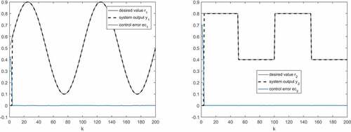
Figure 12. The control law $u_1$ and $u_2$ trajectories.

In this case, both neural network model and pre-processing neural network controller consist of single input, $1$ hidden layer with $28$ nodes, and two output nodes, identically, and variable learning rates of neural network model, ${\eta }_i(k)$, and of neural network controller ${\eta }_{ic}(k)$. The used scaling coefficient is ${\lambda }_i={\lambda }_{c_i}=1$ and ${\epsilon }_i={10}^{-2}$, $i=1:2$.

The input vector of the neural network controller is $x_1={\left[x_{r1}(k),x_{r1}(k-1),x_{r1}(k-2),x_{r2}(k),x_{r2}(k-1),x_{r2}(k-2)\right]}^T$. The influence of the dimensionality reduction in the model error and in the control error is shown in Tables 11 and 12.

Table 11. The influence of the dimensionality reduction in the model error.

	KPCA NN model
${\eta }_i$ $i=1:2$	Variable
$MS{E}_{e_1}$	$5,{4430.10}^{-7}$
$MS{E}_{e_2}$	$8,{1510.10}^{-7}$
$MA{E}_{e_1}$	$2,{4000.10}^{-4}$
$MA{E}_{e_2}$	$1,{3635.10}^{-4}$
$max(e_1)$	$0.0023$
$max(e_2)$	$0.0053$
time (s)	$13,8162$

Table 12. The influence of the dimensionality reduction in the control error.

	KPCA NN controller
${\eta }_{ic}$	Variable
$MS{E}_{e_{1c}}$	$5,{4430.10}^{-7}$
$MS{E}_{e_{2c}}$	$8,{1510.10}^{-7}$
$MA{E}_{e_{1c}}$	$0,0057$
$MA{E}_{e_{2c}}$	$0,0091$
$max(e_{1c})$	$0,4251$
$max(e_{2c})$	$0,5000$
time (s)	$34,7886$

5. Conclusion

In this paper, an online combination between the neural network controller and the KPCA method is proposed and is applied with success in indirect adaptive control. Different kernel functions are tested. For instance, the lowest $MS{E}_e$, $MA{E}_e$, $max(e)$, $MS{E}_{e_c}$, $MA{E}_{e_c}$ and $max(e_c)$ are obtained, and it is proved that the sigmoid kernel function is the best. The effectiveness of the proposed algorithm is successfully applied, firstly, to single-input single-output system, with and without disturbances, and it proved its robustness to reject disturbances and to accelerate the speed of the learning phase of the neural model and neural controller. Second, it is applied to MIMO system and it gives good results.

Disclosure statement

No potential conflict of interest was reported by the authors.

References

- O. Mohareri, R. Dhaouadi, and A.B. Rad, Indirect adaptive tracking control of a nonholonomic mobile robot via neural networks, Neurocomputing 88 (2012), pp. 54–66. doi:10.1016/j.neucom.2011.06.035.
- A.A. Bohari, W.M. Utomo, Z.A. Haron, N.M. Zin, S.Y. Sim, and R.M. Ariff, Speed tracking of indirect field oriented control induction motor using neural network, Procedia Technol. 11 (2013), pp. 141–146. doi:10.1016/j.protcy.2013.12.173.
- S. Slama, A. Errachdi, and M. Benrejeb, Adaptive PID controller based on neural networks for MIMO nonlinear systems, J. Theor. Appl. Inf. Technol. 97 2 (2019), pp. 361–371.
- A. Errachdi and M. Benrejeb, Performance comparison of neural network training approaches in indirect adaptive control, Int. J. Control. Autom. Syst. 16 (3) (2018), pp. 1448–1458. doi:10.1007/s12555-017-0085-3.
- N. Ben, W. Ding, D.A. Naif, and E.A. Fuad, Adaptive neural state-feedback tracking control of stochastic nonlinear switched systems: An average dwell-time method, IEEE Trans. Neural Networks Learn. Syst. 30 (4) (2018), pp. 1076–1087. doi:10.1109/TNNLS.2018.2860944.
- N. Ben, L. Yanjun, Z. Wanlu, L. Haitao, D. Peiyong, and L. Junqing, Multiple lyapunov functions for adaptive neural tracking control of switched nonlinear non-lower-triangular systems, IEEE Trans. Cybern. 99 (2019). doi:10.1109/TCYB.2019.2906372
- P.O. Hoyer and A. HyvUarinen, Independent component analysis applied to feature extraction from colour and stereo images, Network 11 (3) (2000), pp. 191–210. doi:10.1088/0954-898X_11_3_302.
- L.J. Cao, K.S. Chua, W.K. Chong, H.P. Lee, and Q.M. Gu, A comparison of PCA, KPCA and ICA for dimensionality reduction in support vector machine, Neurocomputing 55 (1–2) (2003), pp. 321–336. doi:10.1016/S0925-2312(03)00433-8.
- I. Guyon and A. Eliseeff, An introduction to variable and feature selection, J. Mach. Learn. Res. 3 (2003), pp. 1157–1182.
- J. Weston, S. Mukherjee, O. Chapelle, M. Pontil, T. Poggio, and V.N. Vapnik, Feature selection for SVMs, Adv. Neural Inform. Process. Syst. 13 (2001), pp. 668–674.
- F.E.H. Tay and L.J. Cao, Saliency analysis of support vector machines for feature selection, Neural Network World 2 1 (2001), pp. 153–166.
- F.E.H. Tay and L.J. Cao, A comparative study of saliency analysis and genetic algorithm for feature selection in support vector machines, Intell. Data Anal. 5 (3) (2001), pp. 191–209. doi:10.3233/IDA-2001-5302.
- K. Lee and V. Estivill-Castro, Feature extraction and gating techniques for ultrasonic shaft signal classification, Appl. Soft Comput. 7 (2007), pp. 156–165. doi:10.1016/j.asoc.2005.05.003.
- H. Qinshu, L. Xinen, and X. Shifu, Comparison of PCA and model optimization algorithms for system identification using limited data, J. Appl. Sci. 13, 11 (2013), pp. 2082–2086. doi:10.3923/jas.2013.2082.2086
- R. Zhang, J. Tao, R. Lu, and Q. Jin, Decoupled ARX and RBF neural network modeling using PCA and GA optimization for nonlinear distributed parameter systems, IEEE Trans. Neural Networks Learn. Syst. 29 (2) (2018), pp. 457–469. doi:10.1109/TNNLS.2016.2631481.
- M.L. Wang, X.D. Yan, and H.B. Shi, Spatiotemporal prediction for nonlinear parabolic distributed parameter system using an artificial neural network trained by group search optimization, Neurocomputing 113 (2013), pp. 234–240. doi:10.1016/j.neucom.2013.01.037.
- S. Yin, S.X. Ding, A.H. Abandan Sari, and H.Y. Hao, Data-driven monitoring for stochastic systems and its application on batch process, Int. J. Syst. Sci. 44 (7) (2013), pp. 1366–1376. doi:10.1080/00207721.2012.659708.
- E. Aggelogiannaki and H. Sarimveis, Nonlinear model predictive control for distributed parameter systems using data driven artificial neural network models, Comput. Chem. Eng. 32 (6) (2008), pp. 1225–1237. doi:10.1016/j.compchemeng.2007.05.002.
- M. Madhusmita and H.S. Behera, Kohonen self organizing map with modified K-means clustering For high dimensional data set, Int. J. Appl. Inf. Syst. (IJAIS). 2(3) (2012), pp. 34–39. ( Foundation of Computer Science FCS, New York, USA).
- S. Buchala, N. Davey, T.M. Gale, and R.J. Frank, Analysis of linear and nonlinear dimensionality reduction methods for gender classifcation of face images, Int. J. Syst. Sci. 14 (36) (2005), pp. 931–942. doi:10.1080/00207720500381573.
- M. Lennon, G. Mercier, M.C. Mouchot, and L. Hubert-Moy, Curvilinear component analysis for nonlinear dimensionality reduction of hyperspectral images, Proc. SPIE Image Signal Process Remote Sens. VII 4541 (2001), pp. 157–168.
- N.K. Batmanghelich, B. Taskar, and C. Davatzikos, Generative-discriminative basis learning for medical imaging, IEEE Trans. Med. Imaging 31 (2012), pp. 51–69. doi:10.1109/TMI.2011.2162961.
- L. Van der Mateen, E. Postma, and J. Van den Herik, Dimensionality reduction: A comparative review tilburg centre for creative computing, Tilburg University, LE Tilburg, The Netherlands, 2009.
- K. Kuzniar and M. Zajac, Data pre-processing in the neural network identification of the modified walls natural frequencies, Proceedings of the 19th International Conference on Computer Methods in Mechanics CMM-2011, Warszawa, 9–12 May, 2011, pp. 295–296.
- V.M. Janakiraman, X. Nguyen, and D. Assanis, Nonlinear identification of a gasoline HCCI engine using neural networks coupled with principal component analysis, Appl. Soft Comput. 13 (2013), pp. 2375–2389. doi:10.1016/j.asoc.2013.01.006.
- K. Seerapu and R. Srinivas, Face recognition using robust PCA and radial basis function network, Int. J. Comput. Sci. Commun. Networks 2 5 (2012), pp. 584–589.
- N.M. Peleato, R.L. Legge, and R.C. Andrews, Neural networks for dimensionality reduction of fluorescence spectra and prediction of drinking water disinfection by-products, Water Res. 136 (2018), pp. 84–94. doi:10.1016/j.watres.2018.02.052
- C. Sucheta and K.V. Prema, Effect of dimensionality reduction on performance in artificial neural network for user authentication, 3rd IEEE International Advance Computing Conference (IACC), Ghaziabad, India, 2013.
- G.E. Hinton and R.R. Salakhutdinov, Reducing the dimensionality of data with neural networks, Science 313 (2006), pp. 504–507. doi:10.1126/science.1127647.
- Q. Zhu and C. Li, Dimensionality reduction with input training neural network and its application in chemical process modelling, Chinese J. Chern. Eng. 14 (5) (2006), pp. 597–603. doi:10.1016/S1004-9541(06)60121-3.
- C.-Y. Cheng, -C.-C. Hsu, and M.-C. Chen, Adaptive kernel principal component analysis (KPCA) for monitoring small, Ind. Eng. Chem. Res. 49 (2010), pp. 2254–2262. doi:10.1021/ie900521b.
- C. Chakour, M.F. Harkat, and M. Djeghaba, New adaptive kernel principal component analysis for nonlinear dynamic process monitoring, Appl. Math. Inf. Sci. 9 4 (2015), pp. 1833–1845.
- R. Fezai, M. Mansouri, O. Taouali, M.F. Harkat, and N. Bouguila, Online reduced kernel principal component analysis for process monitoring, Jx 61 (2018), pp. 1–11. doi:10.1016/j.jprocont.2017.10.010.
- Y. Xiao and Y. He, A novel approach for analog fault diagnosis based on neural networks and improved kernel PCA, Neurocomputing 74 (2011), pp. 1102–1115. doi:10.1016/j.neucom.2010.12.003.
- A. Errachdi and M. Benrejeb, On-line identification using radial basis function neural network coupled with KPCA, Int. J. Gen. Syst. 45 7 (2016), pp. 1–15.
- K.N. Reddy and V. Ravi, Differential evolution trained kernel principal component WNN and kernel binary quantile regression: Application to banking, Knowledge-Based Syst. 39 (2013), pp. 45–56. doi:10.1016/j.knosys.2012.10.003.
- I. Klevecka and J. Lelis, Pre-processing of input data of neural networks: The case of forecasting telecommunication network traffic, Telektronikk 104 3/4 (2008), pp. 168–178.
- M. Shirzadeh, A. Amirkhani, A. Jalali, and M.R. Mosavi, An indirect adaptive neural control of a visual-based quadrotor robot for pursuing a moving target, ISA Trans 59 (2015), pp. 290–302. doi:10.1016/j.isatra.2015.10.011.
- S.J. Yoo, J.B. Park, and Y.H. Choi, Indirect adaptive control of nonlinear dynamic systems using self recurrent wavelet neural networks via adaptive learning rates, Inf. Sci. 177 (2007), pp. 3074–3098. doi:10.1016/j.ins.2007.02.009.
- B. Scholkopf and A. Smola, Learning with Kernels, MIT Press, Cambridge, 2002.
- K.S. Narendra and K. Parthasarthy, Identification and control of dynamical systems using neural networks, IEEE Trans. Neural Networks 1 (1) (1990), pp. 4–27. doi:10.1109/72.80202.