Cycle-by-Cycle Combustion Optimisation: Calibration of Data-based Models and Improvements of Computational Efficiency

ABSTRACT

Modern combustion engines require an efficient cycle-by-cycle fuel injection control scheme to optimise the single combustion events during transient operation. The online optimisation of the respective control inputs typically needs accurate while sufficiently simple models of the combustion quantities. Based on a recently presented cycle-by-cycle optimisation scheme with a hybrid model, this paper focuses on two aspects to enhance the accuracy as well as computational efficiency for an online computation. Firstly, the proper calibration of Gaussian processes nested in a combined physics-/data-based model structure is addressed. Respective test bench measurements and a tailored two-step training procedure are presented. Secondly, the computational efficiency of the online cycle-by-cycle optimisation is increased by mapping computationally intensive calculations into the data-based models through offline preprocessing. In addition, a data-driven approximation of the complete optimisation scheme is proposed to further minimise the computational demand. Simulation studies are used to evaluate the performance of these approaches.

KEYWORDS:

• Hybrid model
• model calibration
• combustion optimisation

1. Introduction

Despite the ongoing electrification of the mobility sector, in the near and mid-term future, diesel driven vehicles will still play an important role in public transportation, especially for heavy-duty and off-road applications [1,2]. Thus, increasing the diesel engine efficiency, i.e. decreasing the emitted $\mathrm{C}{\mathrm{O}}_2$, while minimising harmful emissions like nitrogen oxide ($\mathrm{N}{\mathrm{O}}_{\mathrm{x}}$) or soot remains a high priority [3]. Since the transient engine operation offers great optimisation potential, recent governmental legislations enforce diesel engines to fulfil emission limits that were required only for less dynamic scenarios also under highly transient conditions, i.e. Real Driving Emissions (RDE) [4,5].

Focusing on the transient engine operation, sophisticated control schemes aim to optimally regulate the combustion process via the actuated inputs of e.g. the air or the fuel injection system [6,7]. In this field, approaches of cycle-by-cycle control try to optimise the single combustion events during engine transients. For this task, the parameters of the fuel or even water injection [8] are the main manipulated inputs as they directly affect the combustion whereas air system variables, such as intake pressure or oxygen fraction, pertain time-varying boundary conditions [9]. In order to optimally control this system, mathematical models are employed to precisely assess the cross-relations between the various actuated inputs, time-varying conditions, and combustion quantities (emissions and torque). Since accurate physics-based approaches are often too complex for fast-running cycle-by-cycle control schemes, data-based modelling techniques [10–12] are utilised due to their tight mathematical structure [13,14] despite their limited extrapolation capability, e.g., for extreme conditions or unseen transients. Further, also combined physics-/data-based, i.e. hybrid, models [15] are in the scope of research as they aim to unite the advantages of both modelling domains. Based on the modelled relations between the combustion in- and outputs, the actuated signals are determined online or offline through optimisation-based model inversion [11,16,17].

The real-world application of the previously characterised controllers necessitates a consistent calibration of their data-based models as well as a sufficient computational efficiency to satisfy real-time requirements. In detail, the data-based model calibration involves the gathering of reference data that suits the system specifics and the model purpose. Respective approaches discussed in literature range from sophisticated transient measurement procedures to stabilise Homogeneous Charge Compression Ignition [12] towards steady-state approaches to describe the emissions and torque of engines with a conventional combustion [10,18]. According to the discussed concepts, the design of the experiments must also consider the employed data-based modelling approach. In case of neural networks, the authors of [11] e.g. propose a wide-range design with mixed space filling and full factorial parts whereas the local linear models discussed in [10] require a spatially divided concept tailored to their distributed nature. Even if suitable data is available, the overall model structure may further complicate the data-based model generation. For instance, in a hybrid model, the coupling of the physics-/data-based parts must be considered to determine appropriate training data. Respective calibration approaches are yet not widely discussed.

In order to enhance the computational efficiency of cycle-by-cycle control schemes various concepts are discussed in the literature. Approaches of online optimisation are e.g. tuned by their initial conditions (warm vs. cold start), shut-down criteria, or number of iterations [16]. To further reduce the online effort, the optimisation problem is preprocessed offline and the results are stored in surrogate data-based models [11,17,19]. These concepts increase the computational efficiency but also require a suitable sampling of the optimisation problem to properly calibrate the surrogate models. In addition, they shrink the flexibility of the original optimisation as e.g. configurable weights are fixed in the offline solutions. Thus, keeping the online optimisation instead of the data-based approximation but reducing its computational effort through mathematical simplifications seems a promising, yet not well discussed concept.

Following the literature overview, this paper focusses on the calibration of data-based models located in a hybrid model structure and discusses enhancements of the computational efficiency of an online optimisation scheme. The papers’ contributions are based on a cycle-by-cycle combustion control scheme that was previously presented in [20]. This approach adapts the fuel injection pattern cycle-by-cycle and includes a hybrid cylinder chamber model [21] where combined physics-/data-based parts predict the emissions and the indicated mean effective pressure (IMEP) per engine cycle. The calibration of the data-based part gets challenging as e.g. one of the models does not predict an output signal but rather is integrated closed-loop into the state space representation. Therefore, the paper extends a mixed space filling / full factorial measurement design similar to [11] by a two-step calibration procedure that separately generates the state space and output data-based models. Furthermore, the computational effort of the online optimisation is induced by certain pre-calculations, parts of the physic-based model, and an equality constraint. To exclude these elements from the online execution, the paper describes a concept to map their characteristics through offline preprocessing into the data-based models. As a result, they still affect the online optimisation although they are not executed individually any more. In addition, the paper discusses the derivation of a full data-based approximation of the online optimisation scheme while keeping its original flexibility e.g. by preserving configurable weights.

The paper is structured as follows. Section 2 recapitulates the hybrid cylinder chamber model of [21] and its application to the combustion optimisation in [20]. Section 3 introduces a calibration procedure for the data-based parts of the hybrid model scheme and discusses the design of test bench measurements in order to gather appropriate reference data. Section 4 describes measures that reduce the computational effort of the original combustion optimisation through adaptations of the optimisation scheme and the data-based models. Section 5 evaluates these improvements by means of simulation studies and the conclusions are discussed in Section 6.

2. Combustion optimisation with a hybrid cylinder chamber model

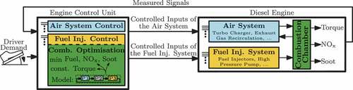
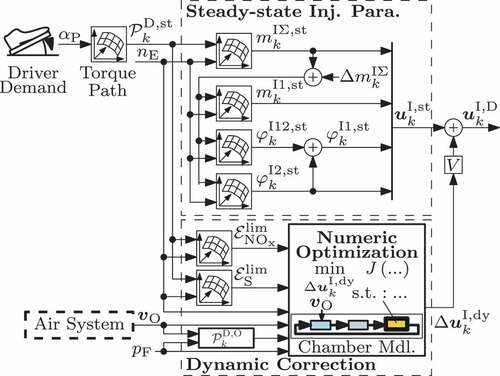
In order to optimally control the combustion during transient engine operation, an optimisation scheme was introduced in [20] to determine correction values for the fuel injection parameters under consideration of their effect on the engine $\mathrm{N}{\mathrm{O}}_{\mathrm{x}}$ and soot emissions as well as on the IMEP. These adaptations are set cycle-by-cycle in reaction to the current air system state and the fuel pressure which are typically delayed during engine transients. The optimisation-based approach thereby extends the standard fuel injection control as depicted in the system overview of Figure 1. In course of the optimisation, the considered engine outputs are determined by a combined physics-/data-based, i.e. hybrid, cylinder chamber description from previous work [21]. Since the current paper discusses the calibration of the data-based model part as well as its utilisation for improving the computational efficiency of the optimisation, this section recapitulates relevant aspects of the initial modelling and control approach. Accordingly, Section 2.1 introduces the hybrid cylinder chamber description and Section 2.2 describes its utilisation for the combustion optimisation.

Figure 1. Overview of the diesel engine structure including the engine control unit.

2.1. Description of the physics-/data-based combustion chamber model

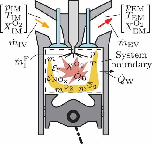
The cylinder chamber modelling approach proposed in [21] transforms a conventional, lumped parameter description concept [22–24] into a hybrid approach that combines physics and data-based models. Thereby, the cylinder interior as well as the gas exchange and fuel injection valves define the balance area boundaries, as indicated by the dashed lines in the cylinder sketch in Figure 2. The model further differentiates between two gas fractions, namely oxygen (${\mathrm{O}}_2$) and the pseudo-component not-oxygen (${\bar{\mathrm{O}}}_2$). Overall, it contains the states

Figure 2. Overview of variables to describe the cylinder chamber.

(1) $\mathit{x}\left(t\right)={\left[\begin{array}{ccc}m\left(t\right)& X^{{\mathrm{O}}_2}\left(t\right)& p\left(t\right)\end{array}\right]}^{\mathrm{T}}$(1)

with the total gas mass $m$, the oxygen faction $X^{{\mathrm{O}}_2}$, and the cylinder pressure $p$.

In detail, the physics-/data-based cylinder chamber description separates the combustion cycle $k$ into the three stages depicted in Figure 3, namely gas exchange (blue), compression (grey) and combustion (yellow). The mathematical representation of this arrangement refers to a periodic hybrid automaton [25] that comprises the mentioned phases as well as their transition events, i.e. exhaust valve opening at $t_k^{\mathrm{E}\mathrm{O}}$, intake valve closing at $t_k^{\mathrm{I}\mathrm{C}}$ and the start of the first fuel injection at $t_k^{\mathrm{I}1}$, see Figure 3. At each transition, the final state of the currently active phase defines the initial state x$0$ of its successor. Except to this requirement, each phase is assumed to be free regarding its specific modelling concept. This generic framework of sequentially connected phases allows to describe the evolution of the cylinder chamber state $\mathit{x}\left(t\right)$ by means of

(2) $\frac{\mathrm{d}\mathfrak{x}(t)}{\mathrm{d}t}=\left\{\begin{array}{c}{\mathit{f}}^{\mathrm{P}1}(t,\mathit{x}(t),{\mathit{v}}_1(t))\mathrm{w}\mathrm{i}\mathrm{t}\mathrm{h}{\mathit{x}}_0=\mathit{x}(t_k^{\mathrm{E}\mathrm{O}})\mathrm{f}\mathrm{o}\mathrm{r}{t}_k^{\mathrm{E}\mathrm{O}}<t\le t_k^{\mathrm{I}\mathrm{C}}(\mathrm{P}\mathrm{h}\mathrm{a}\mathrm{s}\mathrm{e}1)\\ {\mathit{f}}^{\mathrm{P}2}(t,\mathit{x}(t),v_2(t))\mathrm{w}\mathrm{i}\mathrm{t}\mathrm{h}{\mathit{x}}_0=\mathit{x}(t_k^{\mathrm{I}\mathrm{C}})\mathrm{f}\mathrm{o}\mathrm{r}{t}_k^{\mathrm{I}\mathrm{C}}<t\le t_k^{\mathrm{I}1}(\mathrm{P}\mathrm{h}\mathrm{a}\mathrm{s}\mathrm{e}2)\\ \mathrm{u}\mathrm{n}\mathrm{d}\mathrm{e}\mathrm{f}\mathrm{i}\mathrm{n}\mathrm{e}\mathrm{d},(5)\mathrm{a}\mathrm{p}\mathrm{p}\mathrm{r}\mathrm{o}\mathrm{x}\mathrm{i}\mathrm{m}\mathrm{a}\mathrm{t}\mathrm{e}\mathrm{s}\mathit{x}(t_{k+1}^{\mathrm{E}\mathrm{O}})\mathrm{f}\mathrm{o}\mathrm{r}{t}_k^{\mathrm{I}1}<t\le t_{k+1}^{\mathrm{E}\mathrm{O}}(\mathrm{P}\mathrm{h}\mathrm{a}\mathrm{s}\mathrm{e}3).\end{array}\right.$(2)

Figure 3. Hybrid automaton-like structuring of the engine cycle into the gas exchange, compression, and combustion phase.

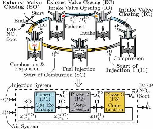
In this approach, the gas exchange and compression phase (phases 1 and 2) are modelled by means of the continuous-time, lumped-parameter cylinder modelling concept [22–24] that is represented by the functions ${\mathit{f}}^{\mathrm{P}1}\left(\cdot \right)$ and ${\mathit{f}}^{\mathrm{P}2}\left(\cdot \right)$, respectively. The input signals

(3) ${\mathit{v}}_1\left(t\right)={\left[\begin{array}{ccccccc}{p}_{\mathrm{I}\mathrm{M}}\left(t\right)& T_{\mathrm{I}\mathrm{M}}\left(t\right)& X_{\mathrm{I}\mathrm{M}}^{{\mathrm{O}}_2}\left(t\right)& p_{\mathrm{E}\mathrm{M}}\left(t\right)& T_{\mathrm{E}\mathrm{M}}\left(t\right)& X_{\mathrm{E}\mathrm{M}}^{{\mathrm{O}}_2}\left(t\right)& n_{\mathrm{E}}\left(t\right)\end{array}\right]}^{\mathrm{T}}$(3)

(4) $v_2(t)=n_{\mathrm{E}}(t)$(4)

of phases 1 and 2 in (2) consider the external air system dependencies, i.e. the thermodynamic states in the intake (IM) and exhaust (EM) manifold, see Figure 2, as well as the engine speed $n_{\mathrm{E}}$. The time-continuous input variables of the gas exchange phase in (3) also enable to attach further models which e.g. describe the air system delay and dead-time effects [26–28].

In contrast to the gas exchange and compression, the complexity of the combustion process requires complex models [29–32] which are, however, inappropriate for the desired combustion optimisation. Thus, at phase 3 in (2), the continuous-time evolution of the states $\mathit{x}(t)$ is substituted by the discrete-time approximation

(5) $\mathit{x}\left(t_{k+1}^{\mathrm{E}\mathrm{O}}\right)\approx {\left[m\left(t_k^{\mathrm{I}1}\right)+m_k^{\mathrm{I}\mathrm{\Sigma }}\hspace{0.17em}\frac{X^{{\mathrm{O}}_2}\left(t_k^{\mathrm{I}1}\right)m\left(t_k^{\mathrm{I}1}\right)-{\mu }_{{\mathrm{O}}_2}{m}_k^{\mathrm{I}\mathrm{\Sigma }}}{m\left(t_k^{\mathrm{I}1}\right)+m_k^{\mathrm{I}\mathrm{\Sigma }}}{\mathcal{M}}_p^{\mathrm{P}3}\left({\gamma }_{\mathcal{M}}^{\mathrm{P}3}\right)\right]}^{\mathrm{T}}$(5)

that only determines the final state x$\left(t_{k+1}^{\mathrm{E}\mathrm{O}}\right)$ of the combustion phase, since it is required for the initialisation of the succeeding gas exchange phase, see Figure 3. In detail, physics-based surrogate models predict the gas mass $m(t_{k+1}^{\mathrm{E}\mathrm{O}})$ and the oxygen fraction $X^{{\mathrm{O}}_2}(t_{k+1}^{\mathrm{E}\mathrm{O}})$. They are derived assuming that the injected fuel mass $m_k^{\mathrm{I}\mathrm{\Sigma }}$ evaporates completely and combusts stoichiometrically with the oxygen demand described by the stoichiometric factor ${\mu }_{{\mathrm{O}}_2}$. Thus, the overall cylinder gas mass $m$ increases and the oxygen fraction $X^{{\mathrm{O}}_2}$ decreases, respectively. Due to the hard-to-describe combustion physics, a more complex, data-based model ${\mathcal{M}}_p^{\mathrm{P}3}\left({\mathit{\gamma }}_{\mathcal{M}}^{\mathrm{P}3}\right)$ determines the cylinder pressure $p(t_{k+1}^{\mathrm{E}\mathrm{O}})$ in (5). Its input vectorγ

(6) ${\gamma }_{\mathcal{M}}^{\mathrm{P}3}=\hspace{0.17em}{\left[\begin{array}{ccccccc}\mathit{x}{\left(t_k^{\mathrm{I}1}\right)}^{\mathrm{T}}& m_k^{\mathrm{I}\mathrm{\Sigma }}& m_k^{\mathrm{I}1}& {\phi }_k^{\mathrm{I}1}& {\phi }_k^{\mathrm{I}2}& p_{\mathrm{F}}\left(t_k^{\mathrm{I}1}\right)& n_{\mathrm{E}}\left(t_k^{\mathrm{I}1}\right)\end{array}\right]}^{\mathrm{T}}$(6)

contains the initial state x$\left(t_k^{\mathrm{I}1}\right)$ calculated by the physics-based model of the compression phase (phase 2) of (2), the fuel injection parameters ${\mathit{u}}_k^{\mathrm{I}}=\hspace{0.17em}{\left[\begin{array}{cccc}{m}_k^{\mathrm{I}\mathrm{\Sigma }}& m_k^{\mathrm{I}1}& {\phi }_k^{\mathrm{I}1}& {\phi }_k^{\mathrm{I}2}\end{array}\right]}^{\mathrm{T}}$ comprising the start positions and fuel mass distribution of the injection impulses according to Figure 4 as well as the fuel pressure $p_{\mathrm{F}}$ and the engine speed $n_{\mathrm{E}}$. These variables are selected as they affect the cylinder pressure evolution during the combustion phase within the governing differential equation. Further, the data-based model ${\mathcal{M}}_p^{\mathrm{P}3}\left({\mathit{\gamma }}_{\mathcal{M}}^{\mathrm{P}3}\right)$ represents a mapping

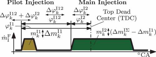
Figure 4. Shape parameter of the fuel mass flow rate and their dynamic correction values.

(7) ${\mathcal{M}}_p^{\mathrm{P}3}\left(\cdot \right):{\gamma }_{\mathcal{M}}^{\mathrm{P}3}\mapsto p\left(t_{k+1}^{\mathrm{E}\mathrm{O}}\right)$(7)

from the input vector ${\mathit{\gamma }}_{\mathcal{M}}^{\mathrm{P}3}\in {\mathbb{R}}^9$ to the scalar pressure signal $p(t_{k+1}^{\mathrm{E}\mathrm{O}})$. Gaussian process regression with a squared exponential kernel [33] is utilised throughout the paper to set up these data-based mappings as it has proven its suitability in the engine modelling domain [13] and is also supported by recent engine control units [34]. The Gaussian process hyper-parameters are estimated by a maximum likelihood approach utilising the software ASCMO (Advanced Simulation for Calibration, Modelling and Optimization) [35].

At each engine cycle $k$, the cylinder chamber model also describes the output signals

(8) ${\mathit{y}}_k={\left[\begin{array}{ccc}\mathcal{P}& {\mathcal{E}}_{\mathrm{N}{\mathrm{O}}_{\mathrm{x}}}& {\mathcal{E}}_{\mathrm{S}}\end{array}\right]}_k^{\mathrm{T}}$(8)

that comprise the IMEP $\mathcal{P}$ as well as the $\mathrm{N}{\mathrm{O}}_{\mathrm{x}}$ and soot emissions ${\mathcal{E}}_{\mathrm{N}{\mathrm{O}}_{\mathrm{x}}}$ and ${\mathcal{E}}_{\mathrm{S}}$. Due to the phase-wise model structure, see Figure 3, and the integral characteristic of the output signals, the vector ${\mathit{y}}_k$ is calculated by the sum

(9) ${\mathit{y}}_k={\mathit{y}}_k^{\mathrm{P}1}+{\mathit{y}}_k^{\mathrm{P}2}+{\mathit{y}}_k^{\mathrm{P}3}$(9)

of the individual contributions

(10) ${\mathit{y}}_k^{\mathrm{P}1}={\left[\begin{array}{ccc}\frac{1}{V_{\mathrm{c}\mathrm{y}\mathrm{l}}}\underset{t_k^{\mathrm{E}\mathrm{O}}}{\overset{t_k^{\mathrm{I}\mathrm{C}}}{\int }}p\left(t\right)\dot{V}\left(t\right)\mathrm{d}t& 0& 0\end{array}\right]}^{\mathrm{T}}$(10)

(11) ${\mathit{y}}_k^{\mathrm{P}2}={\left[\begin{array}{ccc}\frac{1}{V_{\mathrm{c}\mathrm{y}\mathrm{l}}}\underset{t_k^{\mathrm{I}\mathrm{C}}}{\overset{t_k^{\mathrm{I}1}}{\int }}p\left(t\right)\dot{V}\left(t\right)\mathrm{d}t& 0& 0\end{array}\right]}^{\mathrm{T}}$(11)

(12) ${\mathit{y}}_k^{\mathrm{P}3}={\left[\begin{array}{ccc}{\mathcal{M}}_{\mathcal{P}}^{\mathrm{P}3}\left({\mathit{\gamma }}_{\mathcal{M}}^{\mathrm{P}3}\right)& {\mathcal{M}}_{\mathrm{N}{\mathrm{O}}_{\mathrm{x}}}^{\mathrm{P}3}\left({\mathit{\gamma }}_{\mathcal{M}}^{\mathrm{P}3}\right)& {\mathcal{M}}_{\mathrm{S}}^{\mathrm{P}3}\left({\mathit{\gamma }}_{\mathcal{M}}^{\mathrm{P}3}\right)\end{array}\right]}^{\mathrm{T}}$(12)

of each phase. Similar to the state space description (2), the outputs ${\mathit{y}}_k^{\mathrm{P}1}$ and ${\mathit{y}}_k^{\mathrm{P}2}$ of phases 1 and 2 are derived from the physics-based models. In detail, the IMEP is determined from the in-cylinder pressure trace $p(t)$ according to [36]. Further, no emission components are assumed to be aspirated during the gas exchange. Regarding the combustion phase (phase 3), the single elements of ${\mathit{y}}_k^{\mathrm{P}3}$ are determined by the data-based surrogate models ${\mathcal{M}}_{\alpha }^{\mathrm{P}3}\left({\mathit{\gamma }}_{\mathcal{M}}^{\mathrm{P}3}\right),\alpha \in \left\{\mathcal{P},\mathrm{N}{\mathrm{O}}_{\mathrm{x}},\mathrm{S}\right\}$. Similar to (7), they define individual mappings from the input vector ${\mathit{\gamma }}_{\mathcal{M}}^{\mathrm{P}3}\in {\mathbb{R}}^9$ (6) to the respective scalar output signals, which can be summarised in the vector-valued dependency expression

(13) ${\left[\begin{array}{ccc}{\mathcal{M}}_{\mathcal{P}}^{\mathrm{P}3}\left(\cdot \right)& {\mathcal{M}}_{\mathrm{N}{\mathrm{O}}_{\mathrm{x}}}^{\mathrm{P}3}\left(\cdot \right)& {\mathcal{M}}_{\mathrm{S}}^{\mathrm{P}3}\left(\cdot \right)\end{array}\right]}^{\mathrm{T}}:{\mathit{\gamma }}_{\mathcal{M}}^{\mathrm{P}3}\mapsto {\left[\begin{array}{ccc}{\mathcal{P}}^{\mathrm{P}3}& {\mathcal{E}}_{\mathrm{N}{\mathrm{O}}_{\mathrm{x}}}^{\mathrm{P}3}& {\mathcal{E}}_{\mathrm{S}}^{\mathrm{P}3}\end{array}\right]}^{\mathrm{T}}.$(13)

These data-based mappings are also set-up by Gaussian process regression. Thus, they are characterised by the mean values $({\bar{\mathcal{E}}}_{\mathrm{N}{\mathrm{O}}_{\mathrm{x}}},{\bar{\mathcal{E}}}_{\mathrm{S}})$ and standard deviations $({\sigma }_{\mathrm{N}{\mathrm{O}}_{\mathrm{x}}},{\sigma }_{\mathrm{S}})$.

2.2. Fuel injection-based combustion optimisation

The combustion optimisation in [20] determines desired fuel injection parameters ${\mathit{u}}_k^{\mathrm{I},\mathrm{D}}$ that are tailored to the transient engine operation. Therefore, it computes the offsets

(14) $\mathrm{\Delta }{\mathit{u}}_k^{\mathrm{I},\mathrm{d}\mathrm{y}}={\left[\begin{array}{cccc}\mathrm{\Delta }{m}_k^{\mathrm{I}\mathrm{\Sigma }}& \mathrm{\Delta }{m}_k^{\mathrm{I}1}& \mathrm{\Delta }{\phi }_k^{\mathrm{I}12}& \mathrm{\Delta }{\phi }_k^{\mathrm{I}2}\end{array}\right]}^{\mathrm{T}}$(14)

to adapt the steady-state fuel injection parameters

(15) ${\mathit{u}}_k^{\mathrm{I},\mathrm{s}\mathrm{t}}={\left[\begin{array}{cccc}{m}_k^{\mathrm{I}\mathrm{\Sigma },\mathrm{s}\mathrm{t}}& m_k^{\mathrm{I}1,\mathrm{s}\mathrm{t}}& {\phi }_k^{\mathrm{I}1,\mathrm{s}\mathrm{t}}& {\phi }_k^{\mathrm{I}2,\mathrm{s}\mathrm{t}}\end{array}\right]}^{\mathrm{T}}$(15)

under consideration of the actual emission quantities that are e.g. affected negatively by the slow air system and fuel pressure dynamics. Thus, the desired fuel injection parameters for the transient engine operation are calculated on a cycle-by-cycle basis via

(16) ${\mathit{u}}_k^{\mathrm{I},\mathrm{D}}={\mathit{u}}_k^{\mathrm{I},\mathrm{s}\mathrm{t}}+V\mathrm{\Delta }{\mathit{u}}_k^{\mathrm{I},\mathrm{d}\mathrm{y}}.$(16)

This approach considers all degrees of freedom of the two pulse fuel mass flow profile, see Figure 4, i.e. the adaptations $\mathrm{\Delta }{m}_k^{\mathrm{I}\mathrm{\Sigma }}$ and $\mathrm{\Delta }{m}_k^{\mathrm{I}1}$ for the overall and pilot fuel mass, the shift $\mathrm{\Delta }{\phi }_k^{\mathrm{I}2}$ of the main injection start, and $\mathrm{\Delta }{\phi }_k^{\mathrm{I}12}$ for the distance between the pilot and the main injection. To determine the pilot injection shift $\mathrm{\Delta }{\phi }_k^{\mathrm{I}1}$, the conversion matrix $V$ sums up its relative offset $\mathrm{\Delta }{\phi }_k^{\mathrm{I}12}$ and the total shift $\mathrm{\Delta }{\phi }_k^{\mathrm{I}2}$ of the main injection.

The signal scheme in Figure 5 visualises the integration of the correction approach (16) into the standard fuel injection control concept. This section originally determines the steady-state parameters ${\mathit{u}}_k^{\mathrm{I},\mathrm{s}\mathrm{t}}$ via the base maps $f_{\alpha }^{\mathrm{s}\mathrm{t}}(m_k^{\mathrm{I}\mathrm{\Sigma }},n_{\mathrm{E}}),\alpha \in \{m_k^{\mathrm{I}1,\mathrm{s}\mathrm{t}},{\phi }_k^{\mathrm{I}12,\mathrm{s}\mathrm{t}},{\phi }_k^{\mathrm{I}2,\mathrm{s}\mathrm{t}}\}$ in dependence of the total fuel mass $m_k^{\mathrm{I}\mathrm{\Sigma }}$ and the engine speed $n_{\mathrm{E}}$. The offsets $\mathrm{\Delta }{\mathit{u}}_k^{\mathrm{I},\mathrm{d}\mathrm{y}}$ are calculated in addition by the section ”Dynamic Correction“ based on a numeric optimisation approach that utilises the physics-/data-based cylinder chamber model (1)-(13). Further, the optimisation also considers certain $\mathrm{N}{\mathrm{O}}_{\mathrm{x}}$ and soot limits ${\mathcal{E}}_{\mathrm{N}{\mathrm{O}}_{\mathrm{x}}}^{\mathrm{l}\mathrm{i}\mathrm{m}}$ and ${\mathcal{E}}_{\mathrm{S}}^{lim}$, the engine speed $n_{\mathrm{E}}$, the air system coupling variables ${\mathit{v}}_{\mathrm{O}}$, the fuel pressure $p_{\mathrm{F}}$ as well as the desired IMEP ${\mathcal{P}}_k^{\mathrm{D},\mathrm{O}}$. The inputs ${\mathit{v}}_{\mathrm{O}}$ and $p_{\mathrm{F}}$ thereby introduce the current state of the air system and fuel pressure dynamics to the offset calculation.

Figure 5. Extension of the conventional fuel injection control scheme with a dynamic correction approach to improve the transient engine operation.

The actual corrections $\mathrm{\Delta }{\mathit{u}}_k^{\mathrm{I},\mathrm{d}\mathrm{y}}$ (14) are derived by solving the optimisation problem

(17a) $\underset{\mathrm{\Delta }{\mathit{u}}_k^{\mathrm{I},\mathrm{d}\mathrm{y}}\in { }^4}{min}J\left(\begin{array}{ccccc}{\mathcal{E}}_{\mathrm{N}{\mathrm{O}}_{\mathrm{x}},k}^{\mathrm{O}},& {\mathcal{E}}_{\mathrm{N}{\mathrm{O}}_{\mathrm{x}}}^{\mathrm{l}\mathrm{i}\mathrm{m}},& {\mathcal{E}}_{\mathrm{S},k}^{\mathrm{O}},& {\mathcal{E}}_{\mathrm{S}}^{\mathrm{l}\mathrm{i}\mathrm{m}},& m_k^{\mathrm{I}\mathrm{\Sigma },\mathrm{O}}\end{array}\right)$(17a)

(17b) $\mathrm{s}.\mathrm{t}.:\mathrm{P}\mathrm{h}\mathrm{a}\mathrm{s}\mathrm{e}1\mathrm{a}\mathrm{n}\mathrm{d}2\mathrm{o}\mathrm{f}(2)\mathrm{t}\mathrm{o}\mathrm{c}\mathrm{a}\mathrm{l}\mathrm{c}\mathrm{u}\mathrm{l}\mathrm{a}\mathrm{t}\mathrm{e}p(t),t_k^{\mathrm{E}\mathrm{O}}<t\le t_k^{\mathrm{I}1,\mathrm{O}}\mathrm{a}\mathrm{n}\mathrm{d}\mathit{x}(t_k^{\mathrm{I}1,\mathrm{O}})$(17b)

(17c) ${\mathcal{E}}_{\mathrm{N}{\mathrm{O}}_{\mathrm{x}},k}^{\mathrm{O}}={\mathcal{O}}_{\mathrm{N}{\mathrm{O}}_{\mathrm{x}}}^{\mathrm{P}3}\left({\gamma }_{\mathcal{O}}^{\mathrm{P}3}\right)$(17c)

(17d) ${\mathcal{E}}_{\mathrm{S},k}^{\mathrm{O}}={\mathcal{O}}_{\mathrm{S}}^{\mathrm{P}3}\left({\gamma }_{\mathcal{O}}^{\mathrm{P}3}\right)$(17d)

(17e) ${\mathcal{P}}_k^{\mathrm{O}}=\frac{1}{V_{\mathrm{c}\mathrm{y}\mathrm{l}}}\underset{t_k^{\mathrm{E}\mathrm{O}}}{\overset{t_k^{\mathrm{I}\mathrm{C}}}{\int }}p\left(t\right)\dot{V}\left(t\right)\mathrm{d}t+\frac{1}{V_{\mathrm{c}\mathrm{y}\mathrm{l}}}\underset{t_k^{\mathrm{I}\mathrm{C}}}{\overset{t_k^{\mathrm{I}1,\mathrm{O}}}{\int }}p\left(t\right)\dot{V}\left(t\right)\mathrm{d}t+{\mathcal{O}}_{\mathcal{P}}^{\mathrm{P}3}\left({\gamma }_{\mathcal{O}}^{\mathrm{P}3}\right)$(17e)

(17f) $0={\mathcal{P}}_k^{\mathrm{O}}-{\mathcal{P}}_k^{\mathrm{D},\mathrm{O}}$(17f)

(17g) $\mathrm{\Delta }{\mathit{u}}_k^{\mathrm{I},\mathrm{m}\mathrm{i}\mathrm{n}}\le \hspace{0.17em}{\left[\begin{array}{cccc}\mathrm{\Delta }{m}_k^{\mathrm{I}\mathrm{\Sigma }}& \mathrm{\Delta }{m}_k^{\mathrm{I}1}& \mathrm{\Delta }{\phi }_k^{\mathrm{I}12}& \mathrm{\Delta }{\phi }_k^{\mathrm{I}2}\end{array}\right]}^{\mathrm{T}}\le \mathrm{\Delta }{\mathit{u}}_k^{\mathrm{I},\mathrm{m}\mathrm{a}\mathrm{x}}$(17g)

which consists of the objective function (17a) and the constraints (17b)-(17g). In detail, the objective function (17a) has the structure

(18) $J=w_{\mathrm{N}{\mathrm{O}}_{\mathrm{x}}}{\left(max\left\{0,{\bar{\mathcal{E}}}_{\mathrm{N}{\mathrm{O}}_{\mathrm{x}}}^{\mathrm{O}}-{\mathcal{E}}_{\mathrm{N}{\mathrm{O}}_{\mathrm{x}}}^{\mathrm{l}\mathrm{i}\mathrm{m}}\right\}\right)}^2+w_{{\sigma }_{\mathrm{N}{\mathrm{O}}_{\mathrm{x}}}}{\left({\sigma }_{\mathrm{N}{\mathrm{O}}_{\mathrm{x}}}^{\mathrm{O}}\right)}^2$(18)

$+w_{\mathrm{S}}{\left(max\left\{0,{\bar{\mathcal{E}}}_{\mathrm{S}}^{\mathrm{O}}-{\mathcal{E}}_{\mathrm{S}}^{lim}\right\}\right)}^2+w_{{\sigma }_{\mathrm{S}}}{\left({\sigma }_{\mathrm{S}}^{\mathrm{O}}\right)}^2+w_{\mathrm{F}}\left(m_k^{\mathrm{I}\mathrm{\Sigma },\mathrm{s}\mathrm{t}}+\mathrm{\Delta }{m}_k^{\mathrm{I}\mathrm{\Sigma }}\right)$

and thus weights via $w_{\alpha },\alpha \in \{\mathrm{N}{\mathrm{O}}_{\mathrm{x}},{\sigma }_{\mathrm{N}{\mathrm{O}}_{\mathrm{x}}},\mathrm{S},{\sigma }_{\mathrm{S}},\mathrm{F}\}$ between the fuel consumption, the emissions $\mathrm{N}{\mathrm{O}}_{\mathrm{x}}$ and soot as well as their uncertainties (standard deviation). To prevent the optimisation from seeking non-physical results, e.g. zero emissions, the emission quantities are further limited smoothly by means of ${\mathcal{E}}_{\mathrm{N}{\mathrm{O}}_x}^{lim}$ and ${\mathcal{E}}_{\mathrm{S}}^{lim}$. Due to the max function, emissions are only minimised in case they exceed their limit, see Figure 6.

Figure 6. Visualisation of the effect of the $\mathrm{N}{\mathrm{O}}_{\mathrm{x}}$ emission optimisation limit ${\mathcal{E}}_{\mathrm{N}{\mathrm{O}}_{\mathrm{x}}}^{lim}$ in the objective function.

The expressions in (17b)-(17e) comprise the hybrid cylinder chamber model (1)-(13). In detail, (17b) represents the physics-based part, i.e. phases 1 and 2 in (2), and describes the pressure trajectory $p(t)$ in the time interval $t_k^{\mathrm{E}\mathrm{O}}<t\le t_k^{\mathrm{I}1,\mathrm{O}}$ as well as the state x$(t_k^{\text{I}1,\text{O}})$ at the optimised start time $t_k^{\mathrm{I}1,\mathrm{O}}$ of the first fuel injection. The data-based models ${\mathcal{O}}_{\alpha }^{\mathrm{P}3}\left({\mathit{\gamma }}_{\mathcal{O}}^{\mathrm{P}3}\right),\alpha \in \left\{p,\mathcal{P},\mathrm{N}{\mathrm{O}}_{\mathrm{x}},\mathrm{S}\right\}$ in (17b)-(17e) represent the combustion phase approximation in (2) and predict the IMEP ${\mathcal{P}}^{\mathrm{P}3}$, the $\mathrm{N}{\mathrm{O}}_{\mathrm{x}}$ and soot emissions ${\mathcal{E}}_{\mathrm{N}{\mathrm{O}}_{\mathrm{x}}}^{\mathrm{P}3}$ and ${\mathcal{E}}_{\mathrm{S}}^{\mathrm{P}3}$, and the pressure $p(t_{k+1}^{\mathrm{E}\mathrm{O}})$ according to (5) and (12). The identifier $\mathcal{O}$ denotes the utilisation of the data-based models in the optimisation. Their input vector

(19) ${\mathit{\gamma }}_{\mathcal{O}}^{\mathrm{P}3}={\left[\begin{array}{ccccccc}\mathit{x}{(t_k^{\mathrm{I}1,\mathrm{O}})}^{\mathrm{T}}& m_k^{\mathrm{I}\mathrm{\Sigma },\mathrm{O}}& m_k^{\mathrm{I}1,\mathrm{O}}& {\phi }_k^{\mathrm{I}1,\mathrm{O}}& {\phi }_k^{\mathrm{I}2,\mathrm{O}}& p_{\mathrm{F}}& n_{\mathrm{E}}\end{array}\right]}^{\mathrm{T}}$(19)

is derived from (6) and comprises the cylinder state x$(t_k^{\mathrm{I}1,\mathrm{O}})$ calculated by (17b) as well as the optimised fuel injection parameters

(20) ${\left[\begin{array}{cccc}{m}_k^{\mathrm{I}\mathrm{\Sigma },\mathrm{O}}& m_k^{\mathrm{I}1,\mathrm{O}}& {\phi }_k^{\mathrm{I}1,\mathrm{O}}& {\phi }_k^{\mathrm{I}2,\mathrm{O}}\end{array}\right]}^{\mathrm{T}}\widehat{=}{\mathit{u}}_k^{\mathrm{I},\mathrm{O}}$(20)

determined according to (16). Similar to the dependency relation (13), the data-based models ${\mathcal{O}}_{\alpha }^{\mathrm{P}3}({\gamma }_{\mathcal{O}}^{\mathrm{P}3})$ define individual mappings from the input vector ${\gamma }_{\mathcal{O}}^{\mathrm{P}3}\in {\mathbb{R}}^9$ (19) to the scalar outputs, as summarised by

(21) ${\left[\begin{array}{cccc}{\mathcal{O}}_p^{\mathrm{P}3}\left(\cdot \right)& {\mathcal{O}}_{\mathcal{P}}^{\mathrm{P}3}\left(\cdot \right)& {\mathcal{O}}_{\mathrm{N}{\mathrm{O}}_{\mathrm{x}}}^{\mathrm{P}3}\left(\cdot \right)& {\mathcal{O}}_{\mathrm{S}}^{\mathrm{P}3}\left(\cdot \right)\end{array}\right]}^{\mathrm{T}}:{\mathit{\gamma }}_{\mathcal{O}}^{\mathrm{P}3}\mapsto {\left[\begin{array}{cccc}p\left(t_{k+1}^{\mathrm{E}\mathrm{O}}\right)& {\mathcal{P}}^{\mathrm{P}3}& {\mathcal{E}}_{\mathrm{N}{\mathrm{O}}_{\mathrm{x}}}^{\mathrm{P}3}& {\mathcal{E}}_{\mathrm{S}}^{\mathrm{P}3}\end{array}\right]}^{\mathrm{T}}.$(21)

Additionally, the equality constraint in (17f) requires the actual IMEP ${\mathcal{P}}_k^{\mathrm{O}}$ to match the desired IMEP ${\mathcal{P}}_k^{\mathrm{D},\mathrm{O}}$. The actual IMEP ${\mathcal{P}}_k^{\mathrm{O}}$ is determined in (17e) for the current corrections $\mathrm{\Delta }{\mathit{u}}_k^{\mathrm{I},\mathrm{d}\mathrm{y}}$ according to the combined physics-/data-based calculation approach (9). The reference value ${\mathcal{P}}_k^{\mathrm{D},\mathrm{O}}$ is also estimated by means of (9) via

(22) ${\mathcal{P}}_k^{\mathrm{D},\mathrm{O}}=\frac{1}{V_{\mathrm{c}\mathrm{y}\mathrm{l}}}\underset{t_k^{\mathrm{E}\mathrm{O}}}{\overset{t_k^{\mathrm{I}\mathrm{C}}}{\int }}p\left(t\right)\stackrel{.}{V}\left(t\right)dt+\frac{1}{V_{\mathrm{c}\mathrm{y}\mathrm{l}}}\underset{t_k^{1\mathrm{C}}}{\overset{t_k^{\mathrm{I}1,\mathrm{S}\mathrm{t}}}{\int }}p\left(t\right)\stackrel{.}{V}\left(t\right)dt+{\mathcal{O}}_{\mathcal{P}}^{\mathrm{P}3}\left({\gamma }_{\varphi }^{\mathrm{P}3}\right).$(22)

However, the fuel injection parameters are uncorrected, i.e. the steady-state parameters ${\mathit{u}}_k^{\mathrm{I},\mathrm{s}\mathrm{t}}$ are utilised without any offset $\mathrm{\Delta }{\mathit{u}}_k^{\mathrm{I},\mathrm{d}\mathrm{y}}={\left[\begin{array}{cccc}0& 0& 0& 0\end{array}\right]}^{\mathrm{T}}$. Thus, the input vector

(23) ${\gamma }_{\varphi }^{\mathrm{P}3}={\left[\begin{array}{ccccccc}\mathit{x}{\left(t_k^{\mathrm{I}1,\mathrm{s}\mathrm{t}}\right)}^{\mathrm{T}}& m_k^{\mathrm{I}\mathrm{\Sigma },\mathrm{s}\mathrm{t}}& m_k^{\mathrm{I}1,\mathrm{s}\mathrm{t}}& {\phi }_k^{\mathrm{I}1,\mathrm{s}\mathrm{t}}& {\phi }_k^{\mathrm{I}2,\mathrm{s}\mathrm{t}}& p_{\mathrm{F}}& n_{\mathrm{E}}\end{array}\right]}^{\mathrm{T}}$(23)

of the data-based model ${\mathcal{O}}_P^{\mathrm{P}3}\left({\gamma }_{\varphi }^{\mathrm{P}3}\right)$ only considers the steady-state fuel injection properties, which is also indicated by the identifier $\varphi$.

Finally, the inequality constraints (17g) limit the value range of the fuel injection corrections $\mathrm{\Delta }{\mathit{u}}_k^{\mathrm{I},\mathrm{d}\mathrm{y}}$. The upper and lower boundaries

(24) $\mathrm{\Delta }{\mathit{u}}_k^{\mathrm{I},\mathrm{m}\mathrm{i}\mathrm{n}}={\left[\begin{array}{cccc}5\mathrm{m}\mathrm{g}-m_k^{\mathrm{I}\mathrm{\Sigma },\mathrm{s}\mathrm{t}}& -0.5\mathrm{m}\mathrm{g}& -2{}^{\circ }\mathrm{C}\mathrm{A}& -6{}^{\circ }\mathrm{C}\mathrm{A}\end{array}\right]}^{\mathrm{T}}$(24)

(25) $\mathrm{\Delta }{\mathit{u}}_k^{\mathrm{I},\mathrm{m}\mathrm{a}\mathrm{x}}={\left[\begin{array}{cccc}35\mathrm{m}\mathrm{g}-m_k^{\mathrm{I}\mathrm{\Sigma },\mathrm{s}\mathrm{t}}& max\left\{2\mathrm{m}\mathrm{g},3/10m_k^{\mathrm{I}\mathrm{\Sigma },\mathrm{O}}+0.5\mathrm{m}\mathrm{g}\right\}& 6{}^{\circ }\mathrm{C}\mathrm{A}& 6{}^{\circ }\mathrm{C}\mathrm{A}\end{array}\right]}^{\mathrm{T}}$(25)

ensure that the data-based models (21) are utilised only within the training data range discussed in Section 3.3. The fuel mass offset $\mathrm{\Delta }{m}_k^{\mathrm{I}\mathrm{\Sigma }}$ is restricted indirectly such that the resulting total fuel mass $m_k^{\mathrm{I}\mathrm{\Sigma },\mathrm{O}}=m_k^{\mathrm{I}\mathrm{\Sigma },\mathrm{s}\mathrm{t}}+\mathrm{\Delta }{m}_k^{\mathrm{I}\mathrm{\Sigma }}$ maintains the lower and upper boundaries ($5\mathrm{m}\mathrm{g}$ and $35\mathrm{m}\mathrm{g}$) depicted in Figure 9. The limits of the other optimisation variables directly originate from their respective value range in the training data.

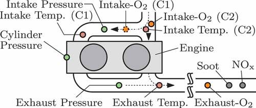
Figure 7. Overview of the test bench structure focussing on the sensors that are located in the intake and exhaust manifold.

3. Generation of data-based models for the combustion optimisation

The combustion optimisation (17) for the transient engine operation utilises the physics-/data-based, i.e. hybrid, cylinder chamber description (1)-(13). The parameters of the physics-based part are typically well known, since they mainly result from geometrical properties. In contrast, the data-based models ${\mathcal{O}}_{\alpha }^{\mathrm{P}3}\left({\mathit{\gamma }}_{\mathcal{O}}^{\mathrm{P}3}\right),\alpha \in \left\{p,\mathcal{P},\mathrm{N}{\mathrm{O}}_{\mathrm{x}},\mathrm{S}\right\}$ require tailored reference data of their in- and output signals to fit the generic Gaussian processes ($\widehat{=}$ training) and evaluate their accuracy ($\widehat{=}$ test). Since steady-state test bench measurements are employed to gather this data, their design needs to ensure that the static models ${\mathcal{O}}_{\alpha }^{\mathrm{P}3}\left({\mathit{\gamma }}_{\mathcal{O}}^{\mathrm{P}3}\right)$ are also valid during engine transients as also discussed in [18,19,37]. The nested location of the data-based models within the hybrid structure further complicates their generation. To solve these issues, Section 3.1 describes a test bench setup that enables the required measurements. Section 3.2 defines the variables to be varied in terms of the measurement campaign while Section 3.3 proposes a concept to shape their variation range. To properly generate the data-based models, Section 3.4 introduces a calibration procedure that processes the steady-state reference data into respective training and test data.

3.1. Description of the test-bench setup

The test-bench setup that is utilised for the gathering of the measurement data comprises all components from the system overview in Figure 1, i.e. an engine control unit, the air and fuel injection system as well as the core engine with an attached electric break to control its speed. Additional test-bench equipment supervises the overall system, controls the measurement procedure, and manages the sensor signal processing. The utilised sensors are visualised in Figure 7. They measure the thermodynamic state in the intake and exhaust manifold, i.e. the pressure, temperature, and oxygen fraction, which also correspond to the air system coupling variables ${\mathit{v}}_{\mathrm{O}}\left(t\right)$ required by the optimisation, see Figure 5. The soot and $\mathrm{N}{\mathrm{O}}_{\mathrm{x}}$ emissions as well as the cylinder pressure trace are also measured by this setup.

Figure 8. Visualisation of the main relations between the air system actuators and the cylinder state $\mathit{x}\left(t_k^{\mathrm{I}1}\right)$ of the data-based model input ${\gamma }_{\mathcal{O}}^{\mathrm{P}3}$.

3.2. Determination of the variation variables

Steady-state test bench measurements are executed to gather reference data for the training and test of the data-based models ${\mathcal{O}}_{\alpha }^{\mathrm{P}3}\left({\gamma }_{\mathcal{O}}^{\mathrm{P}3}\right),\alpha \in \left\{p,\mathcal{P},\mathrm{N}{\mathrm{O}}_{\mathrm{x}},\mathrm{S}\right\}$. To ensure the suitability of the data sets, the measurement design ideally varies the signals

${\left[\begin{array}{ccccccccc}m(t_k^{\mathrm{I}1})& X^{{\mathrm{O}}_2}(t_k^{\mathrm{I}1})& p(t_k^{\mathrm{I}1})& m_k^{\mathrm{I}\mathrm{\Sigma }}& m_k^{\mathrm{I}1}& {\phi }_k^{\mathrm{I}1}& {\phi }_k^{\mathrm{I}2}& p_{\mathrm{F}}& n_{\mathrm{E}}\end{array}\right]}^{\mathrm{T}}$

of their input vector ${\gamma }_{\mathcal{O}}^{\mathrm{P}3}$ (19) in a range that fits to the application in the optimisation. However, due to the limited controllability of certain elements of ${\gamma }_{\mathcal{O}}^{\mathrm{P}3}$, the variables

(26) ${\mathit{\gamma }}_{\mathrm{V}\mathrm{a}\mathrm{r}\mathrm{i}}=\left[\begin{array}{cccccccc}{p}_{\mathrm{I}\mathrm{M}}& X_{\mathrm{I}\mathrm{M}}^{{\mathrm{O}}_2}& m_k^{\mathrm{I}\mathrm{\Sigma }}& m_k^{\mathrm{I}1}& {\phi }_k^{\mathrm{I}1}& {\phi }_k^{\mathrm{I}2}& p_{\mathrm{F}}& n_{\mathrm{E}}\end{array}\right].$(26)

are varied during the test bench measurements. The engine speed $n_{\mathrm{E}}$, the fuel injection parameters ${\mathit{u}}_k^{\mathrm{I}}$, and the fuel pressure $p_{\mathrm{F}}$ are inherited from ${\mathit{\gamma }}_{\mathcal{O}}^{\mathrm{P}3}$ since they can be directly set by the test-bench electric break or the engine control unit. In contrast, no actuators are available to control the cylinder pressure $p(t_k^{\mathrm{I}1})$, gas mass $m(t_k^{\mathrm{I}1})$, and oxygen fraction $X^{{\mathrm{O}}_2}(t_k^{\mathrm{I}1})$. However, the air system actuators enable to set these parameters indirectly, e.g. via the intake manifold conditions. Accordingly, Figure 8 visualises a mapping that shows the main dependencies between the air system actuators and the cylinder filling properties. Thus, the EGR valve is aligned with $X^{{\mathrm{O}}_2}(t_k^{\mathrm{I}1})$ since it affects the intake manifold oxygen fraction $X_{\mathrm{I}\mathrm{M}}^{{\mathrm{O}}_2}$. Similarly, the waste gate valve allows to vary $p(t_k^{\mathrm{I}1})$ by means of the intake pressure $p_{\mathrm{I}\mathrm{M}}$. Since the actual value of $X_{\mathrm{I}\mathrm{M}}^{{\mathrm{O}}_2}$ and $p_{\mathrm{I}\mathrm{M}}$ are measured by the test bench, see Figure 7, respective control loops are established to vary both individually. However, no additional air system actuator is available to set the intake temperature $T_{\mathrm{I}\mathrm{M}}$, and consequentially the gas mass $m(t_k^{\mathrm{I}1,\mathrm{O}})$ independently from the oxygen fraction $X_{\mathrm{I}\mathrm{M}}^{{\mathrm{O}}_2}$ and pressure $p_{\mathrm{I}\mathrm{M}}$. As a result, both induce a certain cylinder gas mass $m(t_k^{\mathrm{I}1,\mathrm{O}})$, which is suboptimal from the measurement design perspective but unavoidable due to the lack of actuators. The previous analysis only considers major dependencies and neglects e.g. the impact of the exhaust manifold state. However, due to the limited number of actuators, they could not be controlled at all.

Figure 9. Visualisation of limits of the variation variables ${\mathit{\gamma }}_{\mathrm{V}\mathrm{a}\mathrm{r}\mathrm{i}}$ and the desired data points (black dots).

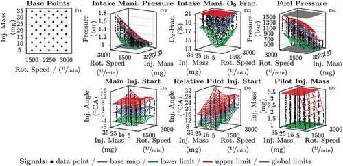
3.3. Design of the parameter variation

The analysis in Section 3.2 defines the signals of ${\gamma }_{\mathrm{V}\mathrm{a}\mathrm{r}\mathrm{i}}$ (26) to be varied during the steady-state test bench measurements to gather reference data for the training and test of the data-based models ${\mathcal{O}}_{\alpha }^{\mathrm{P}3}\left({\gamma }_{\mathcal{O}}^{\mathrm{P}3}\right),\alpha \in \left\{p,\mathcal{P},\mathrm{N}{\mathrm{O}}_{\mathrm{x}},\mathrm{S}\right\}$. Now, this section focuses on the derivation of the data points that are actually tested at the measurement campaign.

To derive the list of samples to be measured, the multidimensional variation space defined by ${\gamma }_{\mathrm{V}\mathrm{a}\mathrm{r}\mathrm{i}}$ must be shaped and filled with data points, respectively. Thus, it needs to be limited to regions aligned with the desired area of application whereas technically inapplicable sections must be dismissed. Accordingly, since the data-based models are utilised in the fuel injection-based combustion optimisation (17), the fuel injection parameters ${\mathit{u}}_k^{\mathrm{I}}$ in ${\mathit{\gamma }}_{\mathrm{V}\mathrm{a}\mathrm{r}\mathrm{i}}$ (26) are varied apart from their base value calibration. Further, the models are intended to be used during transient engine operation. Thus, the variation space also needs to include steady-state operating points that represent the conditions during dynamic engine operation, e.g. in the course of a delayed rise of the intake manifold and fuel pressure after a load step. However, this also pinpoints a limitation of the steady-state measurement concept. If an operation point is only reachable by means of transient engine operation, it cannot be considered.

The diagrams in Figure 9 visualise the variation range of the single elements of ${\mathit{\gamma }}_{\mathrm{V}\mathrm{a}\mathrm{r}\mathrm{i}}$ (26). The black dots represent the desired data points of the measurement procedure. The engine speed and fuel mass in D1 are varied between upper and lower bounds with a slightly modified full factorial design [38], where adjacent data points are shifted to improve space coverage. Further, each engine speed/fuel mass tuple represents a base point at which the remaining variables of ${\mathit{\gamma }}_{\mathrm{V}\mathrm{a}\mathrm{r}\mathrm{i}}$ are varied with a space filling design [38]. The diagrams D2 – D4 of Figure 9 show the variation range of the intake pressure $p_{\mathrm{I}\mathrm{M}}$ (D2) and the oxygen fraction $X_{\mathrm{I}\mathrm{M}}^{{\mathrm{O}}_2}$ (D3) as well as of the fuel pressure $p_{\mathrm{F}}$ (D4). Since all of them exhibit a delayed or overshooting response during engine transients, the purely steady-state measurement procedure also has to cover these regions of operation. Therefore, base maps (blue) describe the standard value of these parameters in dependence of the engine speed $n_{\mathrm{E}}$ and fuel mass $m_k^{\mathrm{I}\mathrm{\Sigma }}$. To cover positive and negative deviations during transient engine operation, the green and red maps up- and downwards of the base values further define a certain variation range. For the intake pressure $p_{\mathrm{I}\mathrm{M}}$ and the fuel pressure $p_{\mathrm{F}}$, the base maps are shifted up- and downwards by a certain offset. However, the positive offset of $p_{\mathrm{I}\mathrm{M}}$ is smaller than the negative for engine safety reasons. During engine transients, the intake oxygen fraction $X_{\mathrm{I}\mathrm{M}}^{{\mathrm{O}}_2}$ may over- or undershoot the base value. Thus, its upper limit in D3 (red) equals the highest possible value, i.e. the fresh air oxygen fraction. The lower limit (green) is derived from prior measurements where the EGR valve is opened step-by-step to determine the minimal oxygen fraction that ensures save engine operation.

The diagrams D5 – D7 of Figure 9 depict the variation design for the fuel injection parameters, namely of the main injection start ${\phi }_k^{\mathrm{I}2}$ in D5, the distance ${\phi }_k^{\mathrm{I}12}$ between the pilot and main injection in D6, and the pilot injection mass $m_k^{\mathrm{I}1}$ in D7. In order to enable the optimisation of the fuel injection parameters, the green and red limit maps define a certain variation range apart from their base values (blue) that correspond to the steady-state fuel injection parameters ${\mathit{u}}_k^{\mathrm{I},\mathrm{s}\mathrm{t}}$. According to Figure 5, the base maps are described by $f_{\alpha }^{\mathrm{s}\mathrm{t}}(m_k^{\mathrm{I}\mathrm{\Sigma }},n_{\mathrm{E}}),\alpha \in \{m_k^{\mathrm{I}1,\mathrm{s}\mathrm{t}},{\phi }_k^{\mathrm{I}12,\mathrm{s}\mathrm{t}},{\phi }_k^{\mathrm{I}2,\mathrm{s}\mathrm{t}}\}$ in dependence of the fuel mass $m_k^{\mathrm{I}\mathrm{\Sigma }}$ and the engine speed $n_{\mathrm{E}}$. For the main injection start, the map is shifted symmetrically by $\pm 6{}^{\circ }\mathrm{C}\mathrm{A}$ (D5). The pilot injection start is varied between $-2{}^{\circ }\mathrm{C}\mathrm{A}$ and $6{}^{\circ }\mathrm{C}\mathrm{A}$ relative to the main injection (D6). The lower limit is smaller than the upper to avoid interactions of the pilot and main injection. Finally, the pilot injection mass is varied between $1\mathrm{m}\mathrm{g}$ and $3.5\mathrm{m}\mathrm{g}$ (D7), whereas for a fuel mass $m_k^{\mathrm{I}\mathrm{\Sigma }}$ below $10\mathrm{m}\mathrm{g}$ its variation range decreases.

The described experiment design comprises full factorial and space filling parameters varied between non-box shaped boundaries. To determine sets of data points that align with these requirements, the toolbox ExpeDes of the software ASCMO [35] is utilised where the space filling design is determined by a Sobol sequence. To increase the robustness against drifts and measurement failures, the test plan contains six sections that independently describe a complete experiment by 275 data points, respectively. This data point amount is a trade-off between the test bench allocation, space coverage, and total model complexity, i.e. the computational effort of the Gaussian processes.

3.4. Calibration of the data-based models

The test bench measurements designed in Section 3.3 intend to generate appropriate reference data to train and test the data-based models ${\mathcal{O}}_{\alpha }^{\mathrm{P}3}\left({\mathit{\gamma }}_{\mathcal{O}}^{\mathrm{P}3}\right),\alpha \in \left\{p,\mathcal{P},\mathrm{N}{\mathrm{O}}_{\mathrm{x}},\mathrm{S}\right\}$ of the combustion optimisation (17). As they are part of the physics-/data-based cylinder chamber model (1)-(13), they are calculated closed-loop with the state space equations of the gas exchange and compression phase. Since this complicates the generation of the data-based models, this section proposes a respective calibration strategy.

The calibration procedure of the data-based models initially assumes, that measurement data is generated in accordance to Section 3.3. The top section in the overview sketch of Figure 10 depicts this prerequisite. Based on this data, the generation of the models ${\mathcal{O}}_{\alpha }^{\mathrm{P}3}(\cdot )$ follows a two-step procedure, as visualised in the lower section of Figure 10. Step one generates the approximation model ${\mathcal{O}}_p^{\mathrm{P}3}(\cdot )$ that determines the cylinder pressure $p(t_{k+1}^{\mathrm{E}\mathrm{O}})$ at the end of the combustion phase. Due to this model, the state space description (2) can be simulated stand-alone. Step two generates the remaining data-based models ${\mathcal{O}}_{\beta }^{\mathrm{P}3}\left({\mathit{\gamma }}_{\mathcal{O}}^{\mathrm{P}3}\right),\beta \in \left\{\mathcal{P},\mathrm{N}{\mathrm{O}}_{\mathrm{x}},\mathrm{S}\right\}$ while the previously built instance of ${\mathcal{O}}_p^{\mathrm{P}3}(\cdot )$ is utilised to simulate the cylinder chamber state x$\hspace{0.17em}$.

Figure 10. Assembly of input-output samples of the training and test data sets at calibration step one and two for the generation of the data-based models ${\mathcal{O}}_{\alpha }^{\mathrm{P}3}\left({\mathit{\gamma }}_{\mathcal{O}}^{\mathrm{P}3}\right),\alpha \in \left\{p,\mathcal{P},\mathrm{N}{\mathrm{O}}_{\mathrm{x}},\mathrm{S}\right\}$ of the optimisation problem (17).

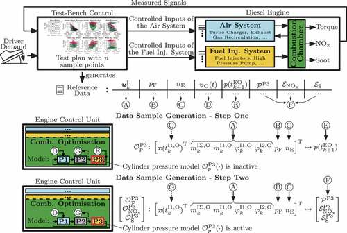
The generation of the data-based models requires training and test data sets. Each of them consists of single samples that comprise signals of the inputs ${\mathit{\gamma }}_{\mathcal{O}}^{\mathrm{P}3}$ and the designated outputs, respectively. The signal flow depicted in Figure 10 visualises the assembly of these data samples at calibration step one and two based on the reference data from test bench measurements. At step one as well as two, the fuel injection parameter ${\mathit{u}}_k^{\mathrm{I}}$ Ⓐ, the fuel pressure $p_{\mathrm{F}}$ Ⓑ and the engine speed $n_{\mathrm{E}}$ Ⓒ of the input vector ${\mathit{\gamma }}_{\mathcal{O}}^{\mathrm{P}3}$ are inherited from the reference data. In contrast, the derivation of the cylinder state x$\left(t_k^{\mathrm{I}1}\right)$ Ⓖ requires the evaluation of the cylinder chamber model, since the respective signals are not provided by the measurement data. To execute the respective simulations, the measured air system coupling variables ${\mathit{v}}_{\mathrm{O}}\left(t\right)$ Ⓓ are required. Further, at step one, the cylinder pressure approximation ${\mathcal{O}}_p^{\mathrm{P}3}(\cdot )$ within phase 3 is not existing yet (phase 3 is crossed out at step one in Figure 10). Thus, the cylinder pressure $p(t_{k+1}^{\mathrm{E}\mathrm{O}})$ at the end of phase 3 is set according to the measured signal Ⓔ. Consequentially, the same signal is also assigned to the output element, since ${\mathcal{O}}_p^{\mathrm{P}3}(\cdot )$ is trained at step one. During the second calibration step, the previously created model ${\mathcal{O}}_p^{\mathrm{P}3}(\cdot )$ enables to simulate the cylinder chamber model in a stand-alone fashion. As a result, the cylinder state $\mathit{x}\left(t_k^{\mathrm{I}1}\right)$ in the input ${\mathit{\gamma }}_{\mathcal{O}}^{\mathrm{P}3}$ of the data-based models ${\mathcal{O}}_{\beta }^{\mathrm{P}3}\left({\mathit{\gamma }}_{\mathcal{O}}^{\mathrm{P}3}\right)$ also contains the unavoidable modelling error that is introduced by the cylinder pressure approximation ${\mathcal{O}}_p^{\mathrm{P}3}(\cdot )$. This ensures data consistency compared to a single-step calibration of all data-based models. At step two, the input vector signals are assembled similar to step one. However, the output values for $\mathrm{N}{\mathrm{O}}_{\mathrm{x}}$, soot, and the IMEP of the combustion phase are inherited from the reference data via Ⓕ, respectively.

The measurement procedure designed in Section 3.3 comprises six sections that independently sample the full range of operation. Three of them are selected for the training and test data, respectively. The sections with the highest share of successful runs are utilised for the training. The symmetric split also considers the computational effort of the Gaussian process regression which scales with the training data size. Overall, the training and test data sets comprise 753 and 524 data points, respectively.

4. Improvements of the computational effort of the combustion optimisation

The fuel injection control concept introduced in Section 2.2 calculates the correction values $\mathrm{\Delta }{\mathit{u}}_k^{\mathrm{I},\mathrm{d}\mathrm{y}}$ for the fuel injection parameters to optimise the combustion during transient engine operation. However, the proposed approach requires the online optimisation problem (17) to be solved, which may be critical w.r.t. the computational power or timing. Accordingly, this section proposes measures to reduce the computational effort of the correction value calculation. Certain adaptations of the optimisation scheme are proposed taking advantage of the flexibility of the data-based models, e.g., to learn further relations in addition to those of their original training data. In detail, Section 4.1 describes a simplifying restructuring of the original optimisation problem (17) that maps certain calculations into the data of the data-based models to remove them from the optimisation scheme. Section 4.2 extends this concept and also projects the IMEP equality constraint (17f) into the data-based models training data. Finally, Section 4.3 proposes an alternative approach that solves the online optimisation problem offline and stores the results in dedicated correction maps.

4.1. Restructuring of the original optimisation problem

The solution of the optimisation problem (17) requires several time-consuming calculations to be performed multiple times. This refers to the physics-based model in (17b) and (17e) that, e.g., determine the state x$(t_k^{\mathrm{I}1,\mathrm{O}})$ and the IMEP ${\mathcal{P}}_k^{\mathrm{P}2,\mathrm{O}}$ of the compression phase (phase 2). In addition, the total fuel injection parameters ${\mathit{u}}_k^{\mathrm{I},\mathrm{O}}$ (20) need to be determined from the steady-state parameters ${\mathit{u}}_k^{\mathrm{I},\mathrm{s}\mathrm{t}}$, which requires the base maps $f_{\alpha }^{\mathrm{s}\mathrm{t}}(m_k^{\mathrm{I}\mathrm{\Sigma }},n_{\mathrm{E}}),\alpha \in \{m_k^{\mathrm{I}1,\mathrm{s}\mathrm{t}},{\phi }_k^{\mathrm{I}12,\mathrm{s}\mathrm{t}},{\phi }_k^{\mathrm{I}2,\mathrm{s}\mathrm{t}}\}$ to be evaluated, see Figure 5. To eliminate this overhead, Section 4.1.1 and 4.1.2 transform the data-based models of the optimisation scheme (17) such that parts of the physics-based model as well as the base maps $f_{\alpha }^{\mathrm{s}\mathrm{t}}(m_k^{\mathrm{I}\mathrm{\Sigma }},n_{\mathrm{E}})$ are mapped into their training data. Section 4.1.3 updates the optimisation problem accordingly. Finally, Section 4.1.4 discusses the accuracy of the updated data-based models.

4.1.1. Substitution of the physics-based calculations of the compression phase

In the optimisation problem (17), the state x$(t_k^{\mathrm{I}1,\mathrm{O}})={\left[\begin{array}{ccc}m(t_k^{\mathrm{I}1,\mathrm{O}})& X^{{\mathrm{O}}_2}(t_k^{\mathrm{I}1,\mathrm{O}})& p(t_k^{\mathrm{I}1,\mathrm{O}})\end{array}\right]}^{\mathrm{T}}$ and the IMEP contribution ${\mathcal{P}}_k^{\mathrm{P}2,\mathrm{O}}$ need to be determined by the physics-based models of the compression phase in (17b) and (17e), respectively. To avoid the explicit calculation of the gas mass $m$ and oxygen fraction $X^{{\mathrm{O}}_2}$ of x$(t_k^{\mathrm{I}1,\mathrm{O}})$, they are defined to equal the state at intake valve closing, i.e. $m(t_k^{\mathrm{I}1,\mathrm{O}})\widehat{=}m(t_k^{\mathrm{I}\mathrm{C}})$ and $X^{{\mathrm{O}}_2}(t_k^{\mathrm{I}1,\mathrm{O}})\widehat{=}{X}^{{\mathrm{O}}_2}(t_k^{\mathrm{I}\mathrm{C}})$. However, this simplification does not apply for the pressure $p(t_k^{\mathrm{I}1,\mathrm{O}})$ and the IMEP ${\mathcal{P}}_k^{\mathrm{P}2,\mathrm{O}}$, since both result from the actual pressure trace $p(t)$ determined by the physics-based model (17b). To substitute these calculations, the approximative data-based mappings

(27) ${\left[\begin{array}{cc}{\mathcal{Z}}_p^{\mathrm{P}2}\left(\cdot \right)& {\mathcal{Z}}_{\mathcal{P}}^{\mathrm{P}2}\left(\cdot \right)\end{array}\right]}^{\mathrm{T}}:{\gamma }_{\mathcal{Z}}^{\mathrm{P}2}\mapsto {\left[\begin{array}{cc}p\left(t_k^{\mathrm{I}1,\mathrm{O}}\right)& {\mathcal{P}}_k^{\mathrm{P}2,\mathrm{O}}\end{array}\right]}^{\mathrm{T}}$(27)

are introduced to directly obtain $p(t_k^{\mathrm{I}1,\mathrm{O}})$ and ${\mathcal{P}}_k^{\mathrm{P}2,\mathrm{O}}$. The input vector

(28) ${\gamma }_{\mathcal{Z}}^{\mathrm{P}2}={\left[\begin{array}{cccc}\mathit{x}{\left(t_k^{\mathrm{I}\mathrm{C}}\right)}^{\mathrm{T}}& m_k^{\mathrm{I}\mathrm{\Sigma },\mathrm{O}}& {\phi }_k^{\mathrm{I}1,\mathrm{O}}& n_{\mathrm{E}}\end{array}\right]}^{\mathrm{T}}$(28)

thereby comprises signals that are aligned with the pressure rise during the compression phase, i.e. the initial cylinder state x$\left(t_k^{\mathrm{I}\mathrm{C}}\right)$, the start ${\phi }_k^{\mathrm{I}1}$ of the pilot injection, the engine speed $n_{\mathrm{E}}$, and the overall fuel mass $m_k^{\mathrm{I}\mathrm{\Sigma }}$. The identifier $\mathcal{Z}$ generally denotes that the physics-based calculations of the compression phase (phase 2) are replaced by the mapping (27). Thus, the cylinder chamber state x$(t_k^{\mathrm{I}1,\mathrm{O}})$ can be approximated by

(29) $\mathit{x}(t_k^{\mathrm{I}1,\mathrm{O}})\approx {\left[\begin{array}{ccc}m\left(t_k^{\mathrm{I}\mathrm{C}}\right)& X^{{\mathrm{O}}_2}\left(t_k^{\mathrm{I}\mathrm{C}}\right)& {\mathcal{Z}}_p^{\mathrm{P}2}\left({\gamma }_{\mathcal{Z}}^{\mathrm{P}2}\right)\end{array}\right]}^{\mathrm{T}}.$(29)

The substitution (29) and the relation ${\mathcal{Z}}_p^{\mathrm{P}2}\left(\cdot \right):{\mathit{\gamma }}_{\mathcal{Z}}^{\mathrm{P}2}\mapsto p(t_k^{\mathrm{I}1,\mathrm{O}})$ from (27) enable to rewrite the input ${\mathit{\gamma }}_{\mathcal{O}}^{\mathrm{P}3}$ (19) of the data-based models ${\mathcal{O}}_{\alpha }^{\mathrm{P}3}\left({\mathit{\gamma }}_{\mathcal{O}}^{\mathrm{P}3}\right),\alpha \in \left\{p,\mathcal{P},\mathrm{N}{\mathrm{O}}_{\mathrm{x}},\mathrm{S}\right\}$ to

(30) ${\gamma }_{\mathcal{Z}}^{\mathrm{P}3}={\left[\begin{array}{ccccccc}\mathit{x}{\left(t_k^{\mathrm{I}\mathrm{C}}\right)}^T& m_k^{\mathrm{I}\mathrm{\Sigma },\mathrm{O}}& m_k^{\mathrm{I}1,\mathrm{O}}& {\phi }_k^{\mathrm{I}1,\mathrm{O}}& {\phi }_k^{\mathrm{I}2,\mathrm{O}}& p_{\mathrm{F}}& n_{\mathrm{E}}\end{array}\right]}^{\mathrm{T}},$(30)

which does not rely any more on the compression phase model to calculate $p(t_k^{\mathrm{I}1,\mathrm{O}})$. This change also requires to update the aligned data-based mappings (21) to

(31) ${\left[\begin{array}{cccc}{\mathcal{Z}}_p^{\mathrm{P}3}\left(\cdot \right)& {\mathcal{Z}}_{\mathrm{N}{\mathrm{O}}_{\mathrm{x}}}^{\mathrm{P}3}\left(\cdot \right)& {\mathcal{Z}}_{\mathrm{S}}^{\mathrm{P}3}\left(\cdot \right)& {\mathcal{Z}}_{\mathcal{P}}^{\mathrm{P}3}\left(\cdot \right)\end{array}\right]}^{\mathrm{T}}:{\gamma }_{\mathcal{Z}}^{\mathrm{P}3}\mapsto {\left[\begin{array}{cccc}p\left(t_{k+1}^{\mathrm{E}\mathrm{O}}\right)& {\mathcal{P}}^{\mathrm{P}3}& {\mathcal{E}}_{\mathrm{N}{\mathrm{O}}_{\mathrm{x}}}^{\mathrm{P}3}& {\mathcal{E}}_{\mathrm{S}}^{\mathrm{P}3}\end{array}\right]}^{\mathrm{T}}.$(31)

Since the cylinder pressure $p(t_k^{\mathrm{I}1})$ is replaced by $p(t_k^{\mathrm{I}\mathrm{C}})$ in ${\gamma }_{\mathcal{Z}}^{\mathrm{P}3}$, the calculations of the physics-based models of phase 2 in (17b) are projected into the data-based models (31).

4.1.2. Substitution of the total fuel injection parameters by their correction values

The previous section introduces the data-based models ${\mathcal{Z}}_{\alpha }^{\mathrm{P}3}\left({\gamma }_{\mathcal{Z}}^{\mathrm{P}3}\right),\alpha \in \left\{p,\mathcal{P},\mathrm{N}{\mathrm{O}}_{\mathrm{x}},\mathrm{S}\right\}$ in (31) and ${\mathcal{Z}}_{\beta }^{\mathrm{P}2}\left({\gamma }_{\mathcal{Z}}^{\mathrm{P}2}\right),\beta \in \left\{\mathcal{P},p\right\}$ in (27), which both avoid computing the physics-based models of the compression phase in (17b) during the optimisation. However, their input vectors ${\gamma }_{\mathcal{Z}}^{\mathrm{P}2}$ (28) and ${\gamma }_{\mathcal{Z}}^{\mathrm{P}3}$ (30) still contain the total fuel injection parameters ${\mathit{u}}_k^{\mathrm{I},\mathrm{O}}$ (20), which require to determine the steady-state parameters ${\mathit{u}}_k^{\mathrm{I},\mathrm{s}\mathrm{t}}$ (15) by the base maps $f_{\nu }^{\mathrm{s}\mathrm{t}}(m_k^{\mathrm{I}\mathrm{\Sigma }},n_{\mathrm{E}}),\nu \in \{m_k^{\mathrm{I}1,\mathrm{s}\mathrm{t}},{\phi }_k^{\mathrm{I}12,\mathrm{s}\mathrm{t}},{\phi }_k^{\mathrm{I}2,\mathrm{s}\mathrm{t}}\}$, see Figure 5. To save this effort, their dependencies should also be mapped into the training data of the data-based models.

At the input vector ${\gamma }_{\mathcal{Z}}^{\mathrm{P}2}$ (28) of the data-based models ${\mathcal{Z}}_{\beta }^{\mathrm{P}2}\left({\gamma }_{\mathcal{Z}}^{\mathrm{P}2}\right)$, the pilot injection start ${\phi }_k^{\mathrm{I}1,\mathrm{O}}$ is a function of the corrected fuel mass $m_k^{\mathrm{I}\mathrm{\Sigma },\mathrm{s}\mathrm{t}}+\mathrm{\Delta }{m}_k^{\mathrm{I}\mathrm{\Sigma }}$, the individual shifts $\mathrm{\Delta }{\phi }_k^{\mathrm{I}2}$ and $\mathrm{\Delta }{\phi }_{\mathrm{k}}^{\mathrm{I}12}$ of the pilot and main injection as well as of the engine speed $n_{\mathrm{E}}$, see Figure 5. These known dependencies enable to rewrite the input vector ${\gamma }_{\mathcal{Z}}^{\mathrm{P}2}$ (28) into

${\gamma }_{\mathcal{Z}}^{\mathrm{P}2}={\left[\begin{array}{cccc}\mathit{x}{\left(t_k^{\mathrm{I}\mathrm{C}}\right)}^{\mathrm{T}}& m_k^{\mathrm{I}\mathrm{\Sigma },\mathrm{O}}& f_{{\phi }_k^{\mathrm{I}1,\mathrm{O}}}\left(m_k^{\mathrm{I}\mathrm{\Sigma },\mathrm{s}\mathrm{t}}+\mathrm{\Delta }{m}_k^{\mathrm{I}\mathrm{\Sigma }},\mathrm{\Delta }{\phi }_k^{\mathrm{I}2},\mathrm{\Delta }{\phi }_k^{\mathrm{I}12},n_{\mathrm{E}}\right)& n_{\mathrm{E}}\end{array}\right]}^{\mathrm{T}}.$

Expanding the dependencies of $f_{{\phi }_k^{\mathrm{I}1,\mathrm{O}}}(\cdot )$ further turns ${\gamma }_{\mathcal{Z}}^{\mathrm{P}2}$ into the vector

(32) ${\gamma }_{\mathcal{Y}}^{\mathrm{P}2}={\left[\begin{array}{ccccc}\mathit{x}{\left(t_k^{\mathrm{I}\mathrm{C}}\right)}^{\mathrm{T}}& \left(m_k^{\mathrm{I}\mathrm{\Sigma },\mathrm{s}\mathrm{t}}+\mathrm{\Delta }{m}_k^{\mathrm{I}\mathrm{\Sigma }}\right)& \mathrm{\Delta }{\phi }_k^{\mathrm{I}12}& \mathrm{\Delta }{\phi }_k^{\mathrm{I}2}& n_{\mathrm{E}}\end{array}\right]}^{\mathrm{T}},$(32)

which does not rely on the total pilot injection start ${\phi }_k^{\mathrm{I}1,\mathrm{O}}$ any more. This is also indicated by the identifier $\mathcal{Y}$. Further, the vector dimension changes from ${\mathbb{R}}^6$ to ${\mathbb{R}}^7$. The input vector ${\mathit{\gamma }}_{\mathcal{Z}}^{\mathrm{P}3}$ (30) of the data-based models ${\mathcal{Z}}_{\alpha }^{\mathrm{P}3}\left({\mathit{\gamma }}_{\mathcal{Z}}^{\mathrm{P}3}\right)$ is transformed similarly. Due to the dependencies of ${\mathit{u}}_k^{\mathrm{I},\mathrm{O}}$ resulting from Figure 5, it is rewritten into

${\gamma }_{\mathcal{Z}}^{\mathrm{P}3}={\left[\begin{array}{cccc}\mathit{x}{\left(t_k^{\mathrm{I}\mathrm{C}}\right)}^{\mathrm{T}}& f_{{\mathit{u}}_k^{\mathrm{I},\mathrm{O}}}\left(m_k^{\mathrm{I}\mathrm{\Sigma },\mathrm{s}\mathrm{t}}+\mathrm{\Delta }{m}_k^{\mathrm{I}\mathrm{\Sigma }},\mathrm{\Delta }{m}_k^{\mathrm{I}1},\mathrm{\Delta }{\phi }_k^{\mathrm{I}12},\mathrm{\Delta }{\phi }_k^{\mathrm{I}2},n_{\mathrm{E}}\right)& p_{\mathrm{F}}& n_{\mathrm{E}}\end{array}\right]}^{\mathrm{T}}.$

After expanding the dependencies of $f_{{\mathit{u}}_k^{\mathrm{I},\mathrm{O}}}(\cdot )$, the input vector ${\gamma }_{\mathcal{Z}}^{\mathrm{P}3}$ turns into

(33) ${\gamma }_{\mathcal{Y}}^{\mathrm{P}3}={\left[\begin{array}{ccccccc}\mathit{x}{(t_k^{\mathrm{I}1,\mathrm{O}})}^{\mathrm{T}}& \left(m_k^{\mathrm{I}\mathrm{\Sigma },\mathrm{s}\mathrm{t}}+\mathrm{\Delta }{m}_k^{\mathrm{I}\mathrm{\Sigma }}\right)& \mathrm{\Delta }{m}_k^{\mathrm{I}1}& \mathrm{\Delta }{\phi }_k^{\mathrm{I}12}& \mathrm{\Delta }{\phi }_k^{\mathrm{I}2}& p_{\mathrm{F}}& n_{\mathrm{E}}\end{array}\right]}^{\mathrm{T}}$(33)

which also just relies on the fuel injection parameter corrections $\mathrm{\Delta }{\mathit{u}}_k^{\mathrm{I},\mathrm{d}\mathrm{y}}$.

Due to the input vector transformations (32) and (33), the steady-state fuel injection parameter ${\mathit{u}}_k^{\mathrm{I},\mathrm{s}\mathrm{t}}$ and consequentially their associated base maps $f_{\nu }^{\mathrm{s}\mathrm{t}}(m_k^{\mathrm{I}\mathrm{\Sigma }},n_{\mathrm{E}})$ must not be evaluated during the optimisation any more. In other words, the transformation inherently integrates the base maps $f_{\nu }^{\mathrm{s}\mathrm{t}}(\cdot )$ into the training data of the data-based models. As a result, the data-based mappings (27) and (31) are updated to

(34) ${\mathcal{Y}}_{\mathcal{P}}^{\mathrm{P}2}\left(\cdot \right):{\gamma }_{\mathcal{Y}}^{\mathrm{P}2}\mapsto {\mathcal{P}}^{\mathrm{P}2}$(34)

(35) ${\left[\begin{array}{cccc}{\mathcal{Y}}_p^{\mathrm{P}3}\left(\cdot \right)& {\mathcal{Y}}_{\mathrm{N}{\mathrm{O}}_{\mathrm{x}}}^{\mathrm{P}3}\left(\cdot \right)& {\mathcal{Y}}_{\mathrm{S}}^{\mathrm{P}3}\left(\cdot \right)& {\mathcal{Y}}_{\mathcal{P}}^{\mathrm{P}3}\left(\cdot \right)\end{array}\right]}^{\mathrm{T}}:{\gamma }_{\mathcal{Y}}^{\mathrm{P}3}\mapsto {\left[\begin{array}{cccc}p\left(t_{k+1}^{\mathrm{E}\mathrm{O}}\right)& {\mathcal{P}}^{\mathrm{P}3}& {\mathcal{E}}_{\mathrm{N}{\mathrm{O}}_{\mathrm{x}}}^{\mathrm{P}3}& {\mathcal{E}}_{\mathrm{S}}^{\mathrm{P}3}\end{array}\right]}^{\mathrm{T}}.$(35)

Since the cylinder pressure mapping ${\mathcal{Z}}_p^{\mathrm{P}2}(\cdot )$ in (27) represented an interims result of Section 4.1.1, it is neglected in (34).

4.1.3. Reformulation of the optimisation problem

Section 4.1.1 and 4.1.2 simplify the optimisation scheme (17) as the physics-based calculations of the compression phase as well as the explicit determination of the steady-state fuel injection parameter ${\mathit{u}}_k^{\mathrm{I},\mathrm{s}\mathrm{t}}$ are both projected into the training data of the data-based models. Accordingly, the optimisation problem (17) is updated to

(36a) $\underset{\mathrm{\Delta }{\mathit{u}}_k^{\mathrm{I},\mathrm{d}\mathrm{y}}\in {\mathbb{R}}^4}{min}J({\mathcal{E}}_{\mathrm{N}{\mathrm{O}}_{\mathrm{X}},k}^{\mathrm{O}},{\mathcal{E}}_{\mathrm{N}{\mathrm{O}}_{\mathrm{X}}}^{lim},{\mathcal{E}}_{\mathrm{S},k}^{\mathrm{O}},{\mathcal{E}}_{\mathrm{S}}^{lim},m_k^{\mathrm{I}\mathrm{\Sigma },\mathrm{O}})$(36a)

(36b) $\mathrm{s}.\mathrm{t}.:\mathrm{P}\mathrm{h}\mathrm{a}\mathrm{s}\mathrm{e}1\mathrm{o}\mathrm{f}(2)\mathrm{t}\mathrm{o}\mathrm{c}\mathrm{a}\mathrm{l}\mathrm{c}\mathrm{u}\mathrm{l}\mathrm{a}\mathrm{t}\mathrm{e}p(t),t_k^{\mathrm{E}\mathrm{O}}<t\le t_k^{\mathrm{I}\mathrm{C}}\mathrm{a}\mathrm{n}\mathrm{d}\mathit{x}(t_k^{\mathrm{I}\mathrm{C}})$(36b)

(36c) ${\mathcal{E}}_{\mathrm{N}{\mathrm{O}}_{\mathrm{x}},k}^{\mathrm{O}}={\mathcal{Y}}_{\mathrm{N}{\mathrm{O}}_{\mathrm{x}}}^{\mathrm{P}3}\left({\gamma }_{\mathcal{Y}}^{\mathrm{P}3}\right)$(36c)

(36d) ${\mathcal{E}}_{\mathrm{S},k}^{\mathrm{O}}={\mathcal{Y}}_{\mathrm{S}}^{\mathrm{P}3}\left({\gamma }_{\mathcal{Y}}^{\mathrm{P}3}\right)$(36d)

(36e) ${\mathcal{P}}_k^{\mathrm{O}}=\frac{1}{V_{\mathrm{c}\mathrm{y}\mathrm{l}}}\underset{t_k^{\mathrm{E}\mathrm{O}}}{\overset{t_k^{\mathrm{I}\mathrm{C}}}{\int }}p\left(t\right)\dot{V}\left(t\right)\mathrm{d}t+{\mathcal{Y}}_{\mathcal{P}}^{\mathrm{P}2}\left({\gamma }_{\mathcal{Y}}^{\mathrm{P}2}\right)+{\mathcal{Y}}_{\mathcal{P}}^{\mathrm{P}3}\left({\gamma }_{\mathcal{Y}}^{\mathrm{P}3}\right)$(36e)

(36f) $0={\mathcal{P}}_k^{\mathrm{O}}-{\mathcal{P}}_k^{\mathrm{D},\mathrm{O}}$(36f)

(36g) $\mathrm{\Delta }{\mathit{u}}_k^{\mathrm{I},\mathrm{m}\mathrm{i}\mathrm{n}}\le {\left[\begin{array}{cccc}\mathrm{\Delta }{m}_k^{\mathrm{I}\mathrm{\Sigma }}& \mathrm{\Delta }{m}_k^{\mathrm{I}1}& \mathrm{\Delta }{\phi }_k^{\mathrm{I}12}& \mathrm{\Delta }{\phi }_k^{\mathrm{I}2}\end{array}\right]}^{\mathrm{T}}\le \mathrm{\Delta }{\mathit{u}}_k^{\mathrm{I},\mathrm{m}\mathrm{a}\mathrm{x}}.$(36g)

The physics-based model part in (36b) now only describes the gas exchange (phase 1) to determine x$\left(t_k^{\mathrm{I}\mathrm{C}}\right)$. Furthermore, the data-based model ${\mathcal{Y}}_{\mathcal{P}}^{\mathrm{P}2}(\cdot )$ calculates the compression phase IMEP ${\mathcal{P}}_k^{\mathrm{P}2,\mathrm{O}}$ in (36e) instead of the physics-based model utilised in (17e).

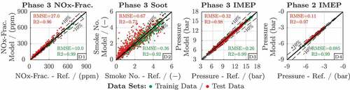
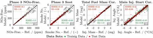
4.1.4. Generation and evaluation of the data-based models

The data-based models ${\mathcal{Y}}_{\alpha }^{\mathrm{P}3}\left({\gamma }_{\mathcal{Y}}^{\mathrm{P}3}\right),\alpha \in \left\{p,\mathcal{P},\mathrm{N}{\mathrm{O}}_{\mathrm{x}},\mathrm{S}\right\}$ and ${\mathcal{Y}}_{\mathcal{P}}^{\mathrm{P}2}$ that are introduced in Section 4.1.2 differ from the models of the original optimisation problem (17). Thus, they need to be generated and tested individually. Their calibration procedure basically follows the approach described in Section 3.4, whereas the input signals of ${\gamma }_{\mathcal{Y}}^{\mathrm{P}3}$ are used instead of ${\gamma }_{\mathcal{O}}^{\mathrm{P}3}$ and the IMEP model ${\mathcal{Y}}_{\mathcal{P}}^{\mathrm{P}2}(\cdot )$ is also trained during step two. The correlation plots in Figure 11 visualise the training (green) and test (red) error of the data-based models that are utilised closed loop in the optimisation. The results for $\mathrm{N}{\mathrm{O}}_{\mathrm{x}}$, soot and the phase 3 IMEP ($\mathrm{D}1-\mathrm{D}3$) are comparable with the results originally discussed in [20]. Further, the newly introduced IMEP model for phase 2 exhibits a small training as well as test data error (D4).

Figure 11. Evaluation of the data-based models ${\mathcal{Y}}_{\alpha }^{\mathrm{P}3}\left({\gamma }_{\mathcal{Y}}^{\mathrm{P}3}\right),\alpha \in \left\{\mathcal{P},\mathrm{N}{\mathrm{O}}_{\mathrm{x}},\mathrm{S}\right\}$ and ${\mathcal{Y}}_{\mathcal{P}}^{\mathrm{P}2}\left({\gamma }_{\mathcal{Y}}^{\mathrm{P}2}\right)$.

4.2. Elimination of the IMEP equality constraint

Section 4.1 introduced several modifications of the original optimisation problem (17) to reduce the calculation overhead. However, the resulting optimisation scheme (36) still requires a certain computational effort to balance the IMEP equality constraint (36f) at each optimisation iteration. Accordingly, Section 4.2.1 proposes to project this constraint into the data of the data-based models such that their prediction inherently satisfy the constraint thus making its explicit consideration superfluous. Section 4.2.2 reformulates the optimisation problem (36) accordingly. Finally, Section 4.2.3 describes the generation and evaluation of the updated data-based models.

4.2.1. Definition of data-based models with inherent IMEP constraint

The IMEP equality constraint (36f) of the optimisation problem (36) requires the actual IMEP ${\mathcal{P}}_k^{\mathrm{O}}$ to match the desired value ${\mathcal{P}}_k^{\mathrm{D},\mathrm{O}}$. According to the governing equation (36e) for ${\mathcal{P}}_k^{\mathrm{O}}$ and (22) for ${\mathcal{P}}_k^{\mathrm{D},\mathrm{O}}$, the constraint (36f) is explicitly described by

(37) $\underset{A}{\underbrace{\frac{1}{V_{\mathrm{c}\mathrm{y}\mathrm{l}}}\hspace{0.17em}\underset{t_k^{IC}}{\overset{t_k^{I1,st}}{\int }}p\left(t\right)\dot{V}\left(t\right)\mathrm{d}t+{\mathcal{O}}_{\mathcal{P}}^{\mathrm{P}3}\left({\gamma }_{\varphi }^{\mathrm{P}3}\right)}}=\underset{B}{\underbrace{{\mathcal{Y}}_{\mathcal{P}}^{\mathrm{P}2}\left({\gamma }_{\mathcal{Y}}^{\mathrm{P}2}\right)+{\mathcal{Y}}_{\mathcal{P}}^{\mathrm{P}3}\left({\gamma }_{\mathcal{Y}}^{\mathrm{P}3}\right)}}.$(37)

The term A, which originates from the desired IMEP ${\mathcal{P}}_k^{\mathrm{D},\mathrm{O}}$ (22), only depends on parameters that are constant during a certain optimisation run, i.e. the cylinder state x$\left(t_k^{\mathrm{I}\mathrm{C}}\right)$ at intake valve closing, the engine speed $n_{\mathrm{E}}$, the fuel pressure $p_{\mathrm{F}}$, and the steady-state fuel injection parameters ${\mathit{u}}_k^{\mathrm{I},\mathrm{s}\mathrm{t}}$. In contrast, term B, which results from the actual IMEP ${\mathcal{P}}_k^{\mathrm{O}}$ (36e), also depends on the optimised injection parameter corrections $\mathrm{\Delta }{\mathit{u}}_k^{\mathrm{I},\mathrm{d}\mathrm{y}}$.

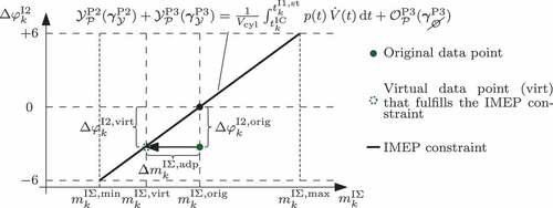
In the course of the optimisation, term A and B of (37) are balanced continuously while the objective function (36a) is minimised. Since the objective purely consists of data-based models, the IMEP constraint may be projected into their training data such that for all of their data points term A and B of (37) are balanced. As the predictions of such data-based models would inherently satisfy the IMEP constraint, its dedicated balancing during the optimisation becomes superfluous.

However, the terms A and B of (37) are unbalanced by default for all training and test data samples created according to Section 3. Hence, a post-processing of the data points is proposed, i.e. a virtual rerun of the test bench measurements, to derive modified samples that inherently satisfy the constraint (37). This data processing approach is visualised in Figure 12. In detail, the fuel mass $m_k^{\mathrm{I}\mathrm{\Sigma },\mathrm{o}\mathrm{r}\mathrm{i}\mathrm{g}}$ of each data sample (green circle) is modified by $\mathrm{\Delta }{m}_k^{\mathrm{I}\mathrm{\Sigma },\mathrm{a}\mathrm{d}\mathrm{p}}$ into the virtual fuel mass $m_k^{\mathrm{I}\mathrm{\Sigma },\mathrm{v}\mathrm{i}\mathrm{r}\mathrm{t}}$ which causes the equality constraint (black line) to be satisfied. In order to preserve the homogeneous, space filling structure of the data sets, the other fuel injection parameters as well as the engine speed $n_{\mathrm{E}}$, fuel pressure $p_{\mathrm{F}}$, and cylinder state x$\left(t_k^{\mathrm{I}\mathrm{C}}\right)$ remain unchanged. Since the modified full mass $m_k^{\mathrm{I}\mathrm{\Sigma },\mathrm{v}\mathrm{i}\mathrm{r}\mathrm{t}}$ changes the emissions, the $\mathrm{N}{\mathrm{O}}_{\mathrm{x}}$ and soot values ${\mathcal{E}}_{\mathrm{N}{\mathrm{O}}_{\mathrm{x}}}$ and ${\mathcal{E}}_{\mathrm{S}}$ of the processed data samples are updated to maintain data consistency. The models ${\mathcal{Y}}_{\mathrm{N}{\mathrm{O}}_{\mathrm{x}}}^{\mathrm{P}3}(\cdot )$ and ${\mathcal{Y}}_{\mathrm{S}}^{\mathrm{P}3}(\cdot )$ from (35) are utilised for these updates.

Figure 12. Concept for processing a data point to inherently satisfy the IMEP constraint equation (37).

The previous data processing introduces a redundancy in the training and test data. Accordingly, the adapted fuel mass $m_k^{\mathrm{I}\mathrm{\Sigma },\mathrm{v}\mathrm{i}\mathrm{r}\mathrm{t}}$ is, e.g., aligned with the shift $\mathrm{\Delta }{\phi }_k^{\mathrm{I}2}$ of the main injection via the desired IMEP

(38) ${\mathcal{P}}_k^{\mathrm{P}23,\varphi }=\frac{1}{V_{\mathrm{c}\mathrm{y}\mathrm{l}}}\underset{t_k^{\mathrm{I}\mathrm{C}}}{\overset{t_k^{\mathrm{I}1,\mathrm{s}\mathrm{t}}}{\int }}p\left(t\right)\dot{V}\left(t\right)\mathrm{d}t+{\mathcal{O}}_{\mathcal{P}}^{\mathrm{P}3}\left({\gamma }_{\varphi }^{\mathrm{P}3}\right),$(38)

that equals term A of (37). The redundancy allows to define the data-based mapping

(39) ${\mathcal{X}}_{m_k^{\mathrm{I}\mathrm{\Sigma }}}^{\mathrm{P}3}\left(\cdot \right):{\gamma }_{\mathcal{X},m_k^{\mathrm{I}\mathrm{\Sigma }}}^{\mathrm{P}3}\mapsto \left(m_k^{\mathrm{I}\mathrm{\Sigma },\mathrm{s}\mathrm{t}}+\mathrm{\Delta }{m}_k^{\mathrm{I}\mathrm{\Sigma }}\right)$(39)

with the input vector

(40) ${\gamma }_{\mathcal{X},m_k^{\mathrm{I}\mathrm{\Sigma }}}^{\mathrm{P}3}={\left[\begin{array}{ccccccc}\mathit{x}{\left(t_k^{\mathrm{I}\mathrm{C}}\right)}^{\mathrm{T}}& {\mathcal{P}}_k^{\mathrm{P}23,\varphi }& \mathrm{\Delta }{m}_k^{\mathrm{I}1}& \mathrm{\Delta }{\phi }_k^{\mathrm{I}12}& \mathrm{\Delta }{\phi }_k^{\mathrm{I}2}& p_{\mathrm{F}}& n_{\mathrm{E}}\end{array}\right]}^{\mathrm{T}}$(40)

to determine the corrected fuel mass $m_k^{\mathrm{I}\mathrm{\Sigma },\mathrm{s}\mathrm{t}}+\mathrm{\Delta }{m}_k^{\mathrm{I}\mathrm{\Sigma }}$ that maintains the desired IMEP ${\mathcal{P}}_k^{\mathrm{P}23,\varphi }$ under consideration of the other fuel injection parameter corrections, the engine speed $n_{\mathrm{E}}$, the fuel pressure $p_{\mathrm{F}}$, and the cylinder state x$\left(t_k^{\mathrm{I}\mathrm{C}}\right)$. The identifier $\mathcal{X}$ indicates that the data of the respective data-based models inherently satisfy the IMEP constraint. The elements of the input vector ${\gamma }_{\mathcal{X},m_k^{I\mathrm{\Sigma }}}^{\mathrm{P}3}$ (40) originate from ${\gamma }_{\mathcal{Y}}^{\mathrm{P}3}$ (33), whereas the fuel mass $m_k^{\mathrm{I}\mathrm{\Sigma },\mathrm{s}\mathrm{t}}+\mathrm{\Delta }{m}_k^{\mathrm{I}\mathrm{\Sigma }}$ is replaced by the desired IMEP ${\mathcal{P}}_k^{\mathrm{P}23,\varphi }$ (38). The redundancy in the data also allows to define the mapping

(41) ${\mathcal{X}}_{\mathrm{\Delta }{\phi }_k^{\mathrm{I}2}}^{\mathrm{P}3}\left(\cdot \right):{\gamma }_{\mathcal{X},\mathrm{\Delta }{\phi }_k^{\mathrm{I}2}}^{\mathrm{P}3}\mapsto \mathrm{\Delta }{\phi }_k^{\mathrm{I}2}$(41)

with the input vector

(42) ${\gamma }_{\mathcal{X},\mathrm{\Delta }{\phi }_k^{\mathrm{I}2}}^{\mathrm{P}3}={\left[\begin{array}{ccccccc}\mathit{x}{\left(t_k^{\mathrm{I}\mathrm{C}}\right)}^{\mathrm{T}}& \left(m_k^{\mathrm{I}\mathrm{\Sigma },\mathrm{s}\mathrm{t}}+\mathrm{\Delta }{m}_k^{\mathrm{I}\mathrm{\Sigma }}\right)& \mathrm{\Delta }{m}_k^{\mathrm{I}1}& \mathrm{\Delta }{\phi }_k^{\mathrm{I}12}& {\mathcal{P}}_k^{\mathrm{P}23,\varphi }& p_{\mathrm{F}}& n_{\mathrm{E}}\end{array}\right]}^{\mathrm{T}}$(42)

to describe the main injection start correction $\mathrm{\Delta }{\phi }_k^{\mathrm{I}2}$ for a certain adapted fuel mass $(m_k^{\mathrm{I}\mathrm{\Sigma },\mathrm{s}\mathrm{t}}+\mathrm{\Delta }{m}_k^{\mathrm{I}\mathrm{\Sigma }})$ and desired IMEP ${\mathcal{P}}_k^{\mathrm{P}23,\varphi }$.

Finally, the data-based models ${\mathcal{Y}}_{\mathrm{N}{\mathrm{O}}_{\mathrm{x}}}^{\mathrm{P}3}\left({\gamma }_{\mathcal{Y}}^{\mathrm{P}3}\right)$ and ${\mathcal{Y}}_{\mathrm{S}}^{\mathrm{P}3}\left({\gamma }_{\mathcal{Y}}^{\mathrm{P}3}\right)$ of the exhaust emissions specified in (35) must be redefined due to the updated data such that their predictions inherently satisfy the IMEP constraint. Their input vector ${\gamma }_{\mathcal{Y}}^{\mathrm{P}3}$ (33) is extended with the redundancy mapping (41) of the main injection start correction $\mathrm{\Delta }{\phi }_k^{\mathrm{I}2}$ leading to

${\gamma }_{\mathcal{Y}}^{\mathrm{P}3}={\left[\begin{array}{ccccccc}\mathit{x}{(t_k^{\mathrm{I}1,\mathrm{O}})}^{\mathrm{T}}& \left(m_k^{\mathrm{I}\mathrm{\Sigma },\mathrm{s}\mathrm{t}}+\mathrm{\Delta }{m}_k^{\mathrm{I}\mathrm{\Sigma }}\right)& \mathrm{\Delta }{m}_k^{\mathrm{I}1}& \mathrm{\Delta }{\phi }_k^{\mathrm{I}12}& {\mathcal{X}}_{\mathrm{\Delta }{\phi }_k^{\mathrm{I}2}}^{\mathrm{P}3}\left({\mathit{\gamma }}_{\mathcal{X},\mathrm{\Delta }{\phi }_k^{\mathrm{I}2}}^{\mathrm{P}3}\right)& p_{\mathrm{F}}& n_{\mathrm{E}}\end{array}\right]}^{\mathrm{T}}.$

The expansion of the dependencies of ${\mathcal{X}}_{\mathrm{\Delta }{\phi }_k^{\mathrm{I}2}}^{\mathrm{P}3}\left({\gamma }_{\mathcal{X},\mathrm{\Delta }{\phi }_k^{\mathrm{I}2}}^{\mathrm{P}3}\right)$ turns the input vector ${\mathit{\gamma }}_{\mathcal{Y}}^{\mathrm{P}3}$ into

(43) ${\gamma }_{\mathcal{X}}^{\mathrm{P}3}={\left[\begin{array}{ccccccc}\mathit{x}{\left(t_k^{\mathrm{I}\mathrm{C}}\right)}^{\mathrm{T}}& \left(m_k^{\mathrm{I}\mathrm{\Sigma },\mathrm{s}\mathrm{t}}+\mathrm{\Delta }{m}_k^{\mathrm{I}\mathrm{\Sigma }}\right)& \mathrm{\Delta }{m}_k^{\mathrm{I}1}& \mathrm{\Delta }{\phi }_k^{\mathrm{I}12}& {\mathcal{P}}_k^{\mathrm{P}23,\varphi }& p_{\mathrm{F}}& n_{\mathrm{E}}\end{array}\right]}^{\mathrm{T}},$(43)

where $\mathrm{\Delta }{\phi }_k^{\mathrm{I}2}$ is substituted with the desired IMEP ${\mathcal{P}}_k^{\mathrm{P}23,\varphi }$. Accordingly, the data-based mappings (35) of the emission predictions are updated to

(44) ${\left[\begin{array}{cc}{\mathcal{X}}_{\mathrm{N}{\mathrm{O}}_{\mathrm{x}}}^{\mathrm{P}3}\left(\cdot \right)& {\mathcal{X}}_{\mathrm{S}}^{\mathrm{P}3}\left(\cdot \right)\end{array}\right]}^{\mathrm{T}}:{\gamma }_{\mathcal{X}}^{\mathrm{P}3}\mapsto {\left[\begin{array}{cc}{\mathcal{E}}_{\mathrm{N}{\mathrm{O}}_{\mathrm{x}}}^{\mathrm{P}3}& {\mathcal{E}}_{\mathrm{S}}^{\mathrm{P}3}\end{array}\right]}^{\mathrm{T}}.$(44)

Due to the data preprocessing approach of Figure 12 and the adapted input vector ${\gamma }_{\mathcal{X}}^{\mathrm{P}3}$ (43), the data-based models ${\mathcal{X}}_{\mathrm{N}{\mathrm{O}}_{\mathrm{x}}}^{\mathrm{P}3}(\cdot )$ and ${\mathcal{X}}_{\mathrm{S}}^{\mathrm{P}3}(\cdot )$ predict emissions that inherently align with the IMEP constraint (36f).

4.2.2. Reformulation of the optimisation problem without IMEP constraint

Section 4.2.1 introduces the data-based models ${\mathcal{X}}_{\mathrm{N}{\mathrm{O}}_{\mathrm{x}}}^{\mathrm{P}3}(\cdot )$ and ${\mathcal{X}}_{\mathrm{S}}^{\mathrm{P}3}(\cdot )$ which provide emission predictions that inherently satisfy the IMEP constraint (36f). Hence, the optimisation problem (36) changes to

(45a) $\underset{\mathrm{\Delta }{\mathit{u}}_k^{\mathrm{I},\mathrm{d}\mathrm{y}}\in {\mathbb{R}}^3}{min}J({\mathcal{E}}_{\mathrm{N}{\mathrm{O}}_{\mathrm{x}},k}^{\mathrm{O}},{\mathcal{E}}_{\mathrm{N}{\mathrm{O}}_{\mathrm{x}}}^{\mathrm{l}\mathrm{i}\mathrm{m}},{\mathcal{E}}_{\mathrm{S},k}^{\mathrm{O}},{\mathcal{E}}_{\mathrm{S}}^{\mathrm{l}\mathrm{i}\mathrm{m}},m_k^{\mathrm{I}\mathrm{\Sigma },\mathrm{O}})$(45a)

(45b) $\mathrm{s}.\mathrm{t}.:\mathrm{P}\mathrm{h}\mathrm{a}\mathrm{s}\mathrm{e}1\mathrm{o}\mathrm{f}(2)\mathrm{t}\mathrm{o}\mathrm{c}\mathrm{a}\mathrm{l}\mathrm{c}\mathrm{u}\mathrm{l}\mathrm{a}\mathrm{t}\mathrm{e}p(t),t_k^{\mathrm{E}\mathrm{O}}<t\le t_k^{\mathrm{I}\mathrm{C}}\mathrm{a}\mathrm{n}\mathrm{d}\mathit{x}(t_k^{\mathrm{I}\mathrm{C}})$(45b)

(45c) ${\mathcal{E}}_{\mathrm{N}{\mathrm{O}}_{\mathrm{x}},k}^{\mathrm{O}}={\mathcal{X}}_{\mathrm{N}{\mathrm{O}}_{\mathrm{x}}}^{\mathrm{P}3}\left({\gamma }_{\mathcal{X}}^{\mathrm{P}3}\right)$(45c)

(45d) ${\mathcal{E}}_{\mathrm{S},k}^{\mathrm{O}}={\mathcal{X}}_{\mathrm{S}}^{\mathrm{P}3}\left({\gamma }_{\mathcal{X}}^{\mathrm{P}3}\right)$(45d)

(45e) $\mathrm{\Delta }{\mathit{u}}_k^{\mathrm{I},\mathrm{m}\mathrm{i}\mathrm{n}}\le {\left[\begin{array}{ccc}\mathrm{\Delta }{m}_k^{\mathrm{I}\mathrm{\Sigma }}& \mathrm{\Delta }{m}_k^{\mathrm{I}1}& \mathrm{\Delta }{\phi }_k^{\mathrm{I}12}\end{array}\right]}^{\mathrm{T}}\le \mathrm{\Delta }{\mathit{u}}_k^{\mathrm{I},\mathrm{m}\mathrm{a}\mathrm{x}}$(45e)

where the IMEP constraint (36f) is excluded. As the main injection correction $\mathrm{\Delta }{\phi }_k^{\mathrm{I}2}$ is substituted by the desired IMEP ${\mathcal{P}}_k^{\mathrm{P}23,\varphi }$ in the input ${\mathit{\gamma }}_{\mathcal{X}}^{\mathrm{P}3}$ (43) of the data-based models ${\mathcal{X}}_{\mathrm{N}{\mathrm{O}}_{\mathrm{x}}}^{\mathrm{P}3}(\cdot )$ and ${\mathcal{X}}_{\mathrm{S}}^{\mathrm{P}3}(\cdot )$, it is also removed from the optimisation variables of (45). However, at the end of each optimisation run, the value of $\mathrm{\Delta }{\phi }_k^{\mathrm{I}2}$ is determined by means of ${\mathcal{X}}_{\mathrm{\Delta }{\phi }_k^{\mathrm{I}2}}^{\mathrm{P}3}(\cdot )$ (41). Hence, the upper and lower limits of $\mathrm{\Delta }{\phi }_k^{\mathrm{I}2}$, i.e. $(-6\le \mathrm{\Delta }{\phi }_k^{\mathrm{I}2}\le +6)$ from (24) and (25), still restrict the optimisation through certain lower and upper bounds $m_k^{\mathrm{I}\mathrm{\Sigma },\mathrm{m}\mathrm{i}\mathrm{n}}$ and $m_k^{\mathrm{I}\mathrm{\Sigma },\mathrm{m}\mathrm{a}\mathrm{x}}$ for the optimised total fuel mass $m_k^{\mathrm{I}\mathrm{\Sigma },\mathrm{s}\mathrm{t}}+\mathrm{\Delta }{m}_k^{\mathrm{I}\mathrm{\Sigma }}$, see also Figure 12. These limits are determined by means of the data-based model ${\mathcal{X}}_{m_k^{\mathrm{I}\mathrm{\Sigma }}}^{\mathrm{P}3}(\cdot )$ (39) with the input vector

(46) ${\gamma }_{\mathcal{X},m_k^{\mathrm{I}\mathrm{\Sigma },\mathrm{m}\mathrm{i}\mathrm{n}}}^{\mathrm{P}3}={\left[\begin{array}{ccccccc}\mathit{x}{\left(t_k^{\mathrm{I}\mathrm{C}}\right)}^{\mathrm{T}}& {\mathcal{P}}_k^{\mathrm{P}23,\varphi }& \mathrm{\Delta }{m}_k^{\mathrm{I}1}& \mathrm{\Delta }{\phi }_k^{\mathrm{I}12}& -6^{\circ }\mathrm{C}\mathrm{A}& p_{\mathrm{F}}& n_{\mathrm{E}}\end{array}\right]}^{\mathrm{T}}$(46)

in order to determine $m_k^{\mathrm{I}\mathrm{\Sigma },\mathrm{m}\mathrm{i}\mathrm{n}}$ and

(47) ${\gamma }_{\mathcal{X},m_k^{\mathrm{I}\mathrm{\Sigma },\mathrm{m}\mathrm{a}\mathrm{x}}}^{\mathrm{P}3}={\left[\begin{array}{ccccccc}\mathit{x}{\left(t_k^{\mathrm{I}\mathrm{C}}\right)}^{\mathrm{T}}& {\mathcal{P}}_k^{\mathrm{P}23,\varphi }& \mathrm{\Delta }{m}_k^{\mathrm{I}1}& \mathrm{\Delta }{\phi }_k^{\mathrm{I}12}& 6^{\circ }\mathrm{C}\mathrm{A}& p_{\mathrm{F}}& n_{\mathrm{E}}\end{array}\right]}^{\mathrm{T}}$(47)

to derive $m_k^{\mathrm{I}\mathrm{\Sigma },\mathrm{m}\mathrm{a}\mathrm{x}}$. In order to consider these restrictions within the constraint (45e), the bounds of $\mathrm{\Delta }{m}_k^{\mathrm{I}\mathrm{\Sigma }}$ from (24) and (25) are adapted to $\mathrm{\Delta }{m}_k^{\mathrm{I}\mathrm{\Sigma },\mathrm{m}\mathrm{i}\mathrm{n}}=m_k^{\mathrm{I}\mathrm{\Sigma },\mathrm{m}\mathrm{i}\mathrm{n}}-m_k^{\mathrm{I}\mathrm{\Sigma },\mathrm{s}\mathrm{t}}$ and $\mathrm{\Delta }{m}_k^{\mathrm{I}\mathrm{\Sigma },\mathrm{m}\mathrm{a}\mathrm{x}}=m_k^{\mathrm{I}\mathrm{\Sigma },\mathrm{m}\mathrm{a}\mathrm{x}}-m_k^{\mathrm{I}\mathrm{\Sigma },\mathrm{s}\mathrm{t}}$, respectively. The limits $m_k^{\mathrm{I}\mathrm{\Sigma },\mathrm{m}\mathrm{i}\mathrm{n}}$ and $m_k^{\mathrm{I}\mathrm{\Sigma },\mathrm{m}\mathrm{a}\mathrm{x}}$ from (46) and (47) thereby inherently consider the global fuel mass bounds $5\mathrm{m}\mathrm{g}$ and $35\mathrm{m}\mathrm{g}$ of (24) and (25). In case only the total fuel mass is optimised via $\mathrm{\Delta }{m}_k^{\mathrm{I}\mathrm{\Sigma }}$, i.e. for $\mathrm{\Delta }{\phi }_k^{\mathrm{I}12}=0{}^{\circ }\mathrm{C}\mathrm{A}$ and $\mathrm{\Delta }{m}_k^{\mathrm{I}1}=0\mathrm{m}\mathrm{g}$, the limits (46) and (47) are constant during an optimisation run. Otherwise, they need to be updated at each optimisation iteration.

4.2.3. Generation and evaluation of the data-based models

The data-based models ${\mathcal{X}}_{\alpha }^{\mathrm{P}3}\left({\gamma }_{\mathcal{X}}^{\mathrm{P}3}\right),\alpha \in \left\{\mathrm{N}{\mathrm{O}}_{\mathrm{x}},\mathrm{S},m_k^{\mathrm{I}\mathrm{\Sigma },\mathrm{O}},\mathrm{\Delta }{\phi }_k^{\mathrm{I}2}\right\}$ introduced in Section 4.2.1 must be generated and tested. In contrast to the previous models, their data is derived by post-processing existing data sets according to Section 4.2.1. The data of the data-based models from Section 4.1.4 is utilised for this purpose.

The correlation diagrams in Figure 13 visualise the training and test data error of the data-based models. The error of $\mathrm{N}{\mathrm{O}}_{\mathrm{x}}$ (D1) and soot (D2) is smaller compared with the previous models ${\mathcal{Y}}_{\alpha }^{\mathrm{P}3}\left({\gamma }_{\mathcal{Y}}^{\mathrm{P}3}\right)$ in Figure 11. This results from the smooth training data, that is derived from sampling ${\mathcal{Y}}_{\mathrm{N}{\mathrm{O}}_{\mathrm{x}}}^{\mathrm{P}3}(\cdot )$ and ${\mathcal{Y}}_{\mathrm{S}}^{\mathrm{P}3}(\cdot )$ according to Section 4.2.1. The redundancy models ${\mathcal{X}}_{m_k^{\mathrm{I}\mathrm{\Sigma }}}^{\mathrm{P}3}(\cdot )$ (D3) and ${\mathcal{X}}_{\mathrm{\Delta }{\phi }_k^{\mathrm{I}2}}^{\mathrm{P}3}(\cdot )$ (D4) also show a small error.

Figure 13. Evaluation of the data-based models ${\mathcal{X}}_{\alpha }^{\mathrm{P}3}\left({\gamma }_{\mathcal{X}}^{\mathrm{P}3}\right),\alpha \in \left\{\mathrm{N}{\mathrm{O}}_{\mathrm{x}},\mathrm{S},m_k^{\mathrm{I}\mathrm{\Sigma },\mathrm{O}},\mathrm{\Delta }{\phi }_k^{\mathrm{I}2}\right\}$.

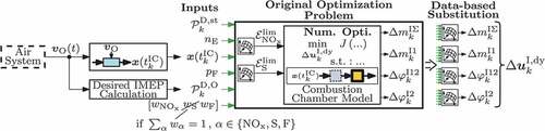
4.3. Offline learning of the optimisation results

The previous Sections 4.1 and 4.2 introduce approaches to minimise the computational effort of the original optimisation problem (17). However, instead of solving it online during runtime, the following approach determines the corrections $\mathrm{\Delta }{\mathit{u}}_k^{\mathrm{I},\mathrm{d}\mathrm{y}}$ offline and stores the results in respective data-based surrogate models, as depicted in the signal flow diagram in Figure 14. To establish this concept, Section 4.3.1 proposes an input-output structure for these correction models that also preserves the flexibility of the original optimisation problem, e.g., regarding variable weights. As different types can be created, Section 4.3.2 describes the variants investigated by this paper. Finally, Section 4.3.3 describes the generation and evaluation of the surrogate correction models.

Figure 14. Concept for deriving data-based models that substitute the online optimisation to determine the fuel injection correction $\mathrm{\Delta }{\mathit{u}}_k^{\mathrm{I},\mathrm{d}\mathrm{y}}$.

4.3.1. Definition of data-based models for the fuel injection parameter corrections

In order to derive data-based models that substitute the optimisation (17), a set of input signals ${\gamma }_{\mathcal{W}}$ must be defined to unambiguously describe the correction values $\mathrm{\Delta }{\mathit{u}}_k^{\mathrm{I},\mathrm{d}\mathrm{y}}$. These signals are selected according to the external dependencies of the original optimisation problem (17) depicted in Figure 5. In the left part of the diagram in Figure 14, these relations are restructured to derive the signals

(48) ${\gamma }_{\mathcal{W}}={\left[\begin{array}{ccccccc}\mathit{x}{\left(t_k^{\mathrm{I}\mathrm{C}}\right)}^{\mathrm{T}}& {\mathcal{P}}_k^{\mathrm{D},\mathrm{s}\mathrm{t}}& {\mathcal{P}}_k^{\mathrm{D},\mathrm{O}}& n_{\mathrm{E}}& p_{\mathrm{F}}& w_{\mathrm{N}{\mathrm{O}}_{\mathrm{x}}}& w_{\mathrm{F}}\end{array}\right]}^{\mathrm{T}}$(48)

that specify the external dependencies of (17). Hence, both IMEP set points ${\mathcal{P}}_k^{\mathrm{D},\mathrm{O}}$ and ${\mathcal{P}}_k^{\mathrm{D},\mathrm{s}\mathrm{t}}$, the cylinder filling properties x$\left(t_k^{\mathrm{I}\mathrm{C}}\right)$ at intake valve closing, the engine speed $n_{\mathrm{E}}$, the fuel pressure $p_{\mathrm{F}}$, and the weights of the objective function (18) are required. For reasons of simplicity, the weights $w_{{\sigma }_{\mathrm{N}{\mathrm{O}}_{\mathrm{x}}}}$ and $w_{{\sigma }_{\mathrm{S}}}$ of the model uncertainty terms are neglected. Consequently, the data-based mappings

(49) ${\left[\begin{array}{cccc}{\mathcal{W}}_{\mathrm{\Delta }{m}_k^{\mathrm{I}\mathrm{\Sigma }}}\left(\cdot \right)& {\mathcal{W}}_{\mathrm{\Delta }{m}_k^{\mathrm{I}1}}\left(\cdot \right)& {\mathcal{W}}_{\mathrm{\Delta }{\phi }_k^{\mathrm{I}12}}\left(\cdot \right)& {\mathcal{W}}_{\mathrm{\Delta }{\phi }_k^{\mathrm{I}2}}\left(\cdot \right)\end{array}\right]}^{\mathrm{T}}:{\gamma }_{\mathcal{W}}\mapsto {\left[\begin{array}{cccc}\mathrm{\Delta }{m}_k^{\mathrm{I}\mathrm{\Sigma }}& \mathrm{\Delta }{m}_k^{\mathrm{I}1}& \mathrm{\Delta }{\phi }_k^{\mathrm{I}12}& \mathrm{\Delta }{\phi }_k^{\mathrm{I}2}\end{array}\right]}^{\mathrm{T}}$(49)

can be defined to explicitly describe the fuel injection corrections $\mathrm{\Delta }{\mathit{u}}_k^{\mathrm{I},\mathrm{d}\mathrm{y}}$. The identifier $\mathcal{W}$ denotes that these data-based models substitute the online optimisation.

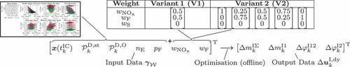
4.3.2. Derivation of the data for the data-based correction models

The generation of the substituting data-based models (49) requires certain training and test data. According to Section 3.3, such data sets must contain data samples that vary the input signals ${\gamma }_{\mathcal{W}}$ in a meaningful range and also provide the output signals, i.e. the fuel injection parameter corrections $\mathrm{\Delta }{\mathit{u}}_k^{\mathrm{I},\mathrm{d}\mathrm{y}}$. In contrast to the data-based models utilised in the original optimisation problem (17), this input-output data does not originate from measurement data, but from sampling (17) for various boundary conditions. The sketch in Figure 15 shows the concept that is utilised to perform this sampling of the optimisation scheme. Since the data derived according to Section 3.3 already contains a strong variation of the air system conditions, engine speed, fuel pressure, and load, it is used to define a base variation for the boundary conditions of the optimisation. Further, at each data point, the weights are varied in addition. Within this paper, the weight sampling variants V1 and V2 depicted in Figure 15 are investigated. V1 considers a single weight case where $\mathrm{N}{\mathrm{O}}_{\mathrm{x}}$ and fuel mass are equally prioritised. In contrast, V2 considers multiple combinations of different $\mathrm{N}{\mathrm{O}}_{\mathrm{x}}$ and fuel mass weights. For each of the resulting samples of the input ${\gamma }_{\mathcal{W}}$, the optimisation problem (17) is solved in order to determine the corresponding fuel injection corrections $\mathrm{\Delta }{\mathit{u}}_k^{\mathrm{I},\mathrm{d}\mathrm{y}}$.

Figure 15. Sampling concept of the optimisation problem to derive training and test data for the data-based models ${\mathcal{W}}_{\alpha }\left({\mathit{\gamma }}_{\mathcal{W}}\right),\alpha \in \left\{\mathrm{\Delta }{m}_k^{\mathrm{I}\mathrm{\Sigma }},\mathrm{\Delta }{m}_k^{\mathrm{I}1},\mathrm{\Delta }{\phi }_k^{\mathrm{I}12},\mathrm{\Delta }{\phi }_k^{\mathrm{I}2}\right\}$. The weight variation cases V1 and V2 are investigated.

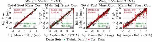
4.3.3. Generation and evaluation of the data-based models

As Section 4.3.2 proposes an approach to determine the training and test data for the data-based correction models (49), this section focusses on their generation and evaluation. In detail, individual models based on Gaussian process regression are created for the weight variants V1 and V2 of Figure 15. Further, only correction models for the main injection shift $\mathrm{\Delta }{\phi }_k^{\mathrm{I}2}$ and the fuel mass offset $\mathrm{\Delta }{m}_k^{\mathrm{I}\mathrm{\Sigma }}$ are generated, since both were identified by [20] as the dominant degrees of freedom of the combustion optimisation.

The correlation plots in Figure 16 visualise the training and test data error of the models ${\mathcal{W}}_{\mathrm{\Delta }{m}_k^{\mathrm{I}\mathrm{\Sigma }}}(\cdot )$ (D1)/(D3) and ${\mathcal{W}}_{\mathrm{\Delta }{\phi }_k^{\mathrm{I}2}}(\cdot )$ (D2)/(D4) for the weight variants V1 and V2, respectively. Overall, the error measures indicate that all models are fitted very well. However, both weight variants show an increased local error in case no corrections are requested, i.e. in the region of $\mathrm{\Delta }{m}_k^{\mathrm{I}\mathrm{\Sigma }}=0$ or $\mathrm{\Delta }{\phi }_k^{\mathrm{I}2}=0$, as well as if the main injection shift $\mathrm{\Delta }{\phi }_k^{\mathrm{I}2}$ is limited by its lower or upper boundary (17g). Since the fuel injection corrections turn into constant values, i.e. flat surfaces, in these regions, the Gaussian process regression obviously has difficulties to accurately describe that behaviour.

Figure 16. Evaluation of the data-based models ${\mathcal{W}}_{\beta }({\gamma }_{\mathcal{W}}),\beta \in \left\{\mathrm{\Delta }{m}_k^{\mathrm{I}\mathrm{\Sigma }},\mathrm{\Delta }{\phi }_k^{\mathrm{I}2}\right\}$ of the weight variation cases V1 and V2.

5. Simulation-based evaluation of the improvements in the computational efficiency of the combustion optimisation

Section 4 introduces several concepts to improve the computational efficiency of the fuel injection-based combustion optimisation (17). This section analyses and compares their effects on the accuracy of the fuel injection control as well as on the time required to determine the corrections values $\mathrm{\Delta }{\mathit{u}}_k^{\mathrm{I},\mathrm{d}\mathrm{y}}$.

The comparison is realised in the simulation-based test-bench environment introduced in [20]. Thus, all tested variants are implemented in Simulink via embedded function blocks. Further, the optimisation-based approaches are solved by the Matlab function fmincon with the interior point algorithm. The Gaussian process models are generated by the software ASCMO [35] and are executed as m-code. The run time that is referred to by the following analysis represents the time needed to determine the fuel injection parameter offsets, e.g. via fmincon or the data-based correction models. This measure excludes the effort of the gas exchange calculations since they are executed equally by each approach once per cycle prior to the correction value calculation. In a standard, non-optimised Simulink environment this model part requires $\approx 0.6\mathrm{s}$ to run.

The different variants of the combustion optimisation are compared at a certain transient test cycle. Its engine speed and accelerator pedal trajectory is depicted in the diagrams D7 and D8 of the simulation results overview in Figure 17. In detail, the engine speed rises as the accelerator pedal is pushed for a certain period of time. The remaining subplots of Figure 17 visualise simulation results, i.e. the emissions and the IMEP generated by cylinder 1 (D1) – (D3), the optimised fuel injection parameters (D4) – (D5) as well as timing measures for the optimisation procedure in D6 and D9.

Figure 17. Comparison of the speed-up measures for the optimisation problem (17). ¹⁾ Each approach also simulates the gas exchange phase once per cycle which requires $\approx 0.6\mathrm{s}$ in addition.

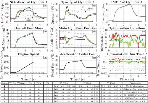
The coloured lines in the plots of Figure 17 indicate the different evaluation cases. Their properties are summarised in the table below the plots. Thus, all variants are configured with the same weight configuration, which equally prioritises $\mathrm{N}{\mathrm{O}}_{\mathrm{x}}$ and fuel mass. In detail, the black case represents a reference at which the fuel injection parameters are not optimised. The red line shows the behaviour in case the corrections $\mathrm{\Delta }{\mathit{u}}_k^{\mathrm{I},\mathrm{d}\mathrm{y}}$ are calculated according to (36) where certain computational overhead is reduced compared to the original formulation (17). The light and dark green cases both visualise the simulation results of the optimisation problem (45), which utilises data-based models that inherently contain the IMEP constraint. The light green case additionally shows the performance of a warm start procedure, i.e. the optimisation is initialised with the final results of the previous run. The light and dark blue cases both represent approaches where the considered fuel injection adaptations $\mathrm{\Delta }{\mathit{u}}_k^{\mathrm{I},\mathrm{d}\mathrm{y}}$ are determined by the purely data-based correction maps (49). The dark blue line corresponds to the weight variation case V1 of Figure 15, i.e. it is generated with the data of only one weight configuration. In contrast, the light blue line corresponds to variant V2 which is trained with data from multiple weight configurations.

As the red case in Figure 17 nearly equals the original optimisation formulation (17), it shows the expected behaviour of the combustion optimisation. In the first section, which is marked by the dotted lines (…) in the subplot of Figure 17, the overall injected fuel mass is decreased by $4\mathrm{\%}$ compared to the black case. However, to maintain the IMEP, the main injection start position is shifted forward, since the non-optimised $\mathrm{N}{\mathrm{O}}_{\mathrm{x}}$ fraction is below its limit ${\mathcal{E}}_{\mathrm{N}{\mathrm{O}}_{\mathrm{x}}}^{\mathrm{l}\mathrm{i}\mathrm{m}}$ (D1). As a result, the emitted $\mathrm{N}{\mathrm{O}}_{\mathrm{x}}$ mass increases by $25\mathrm{\%}$. In the second cycle section, which is marked by (- -), the main injection start is mainly shifted backwards compared with the black reference curve in order to decrease the high $\mathrm{N}{\mathrm{O}}_{\mathrm{x}}$ emissions. To maintain the IMEP, the fuel mass is increased accordingly. As a result, the emitted $\mathrm{N}{\mathrm{O}}_{\mathrm{x}}$ mass decreases by $9\mathrm{\%}$ while the fuel mass increases by $4\mathrm{\%}$. Overall, $5\mathrm{\%}$$\mathrm{N}{\mathrm{O}}_{\mathrm{x}}$ is saved with a $3\mathrm{\%}$ higher invest of fuel mass. Even if soot is neglected by the optimisation due to its zero weight ($w_{\mathrm{S}}=0$), the soot mass is reduced by $2\mathrm{\%}$. On average, a single optimisation run requires $285\mathrm{m}\mathrm{s}$.

The optimisation results of the green coloured cases, where the IMEP constraint is projected into the data-based models, equal those of the red case very well. Particularly, the IMEP trajectory (D3) remains unchanged. However, both require fewer iterations at each optimisation run (D6). The warm start approach (light green) even further reduces the iteration count and in consequence the overall run time required by the optimisation (D9). Compared to the red reference, the average optimisation run time decreases by $56.9\mathrm{\%}$ for the dark green case and $64.9\mathrm{\%}$ for the light green variant.

The light and dark blue cases, which both utilise purely data-based correction maps to calculate $\mathrm{\Delta }{\mathit{u}}_k^{\mathrm{I},\mathrm{d}\mathrm{y}}$, cause slightly different simulation results compared with the red and both green cases. Particularly, in the middle of the first section (---) as well as at the end of the second (- -), the determined fuel injection parameter corrections deviate from those of the online optimisation approaches. However, the total reduction of $\mathrm{N}{\mathrm{O}}_{\mathrm{x}}$ by $4\mathrm{\%}$ and the fuel mass increase of $2\mathrm{\%}$ or $3\mathrm{\%}$ are nearly equal to the cases with online optimisation. In contrast, the run time (D9) decreases significantly, i.e. the average duration of the light blue case is $86.1\mathrm{\%}$ below the time required by the light green variant. The dark blue case, which comprises data-based models that are especially tailored for the currently tested weights $w_{\mathrm{N}{\mathrm{O}}_{\mathrm{x}}}=w_{\mathrm{F}}=0.5$, see V1 in Figure 15, is even $79.1\mathrm{\%}$ faster compared with the light blue variant. The data-based models of the dark blue case are more complex since they also support weight factor combinations that differs from $w_{\mathrm{N}{\mathrm{O}}_{\mathrm{x}}}=w_{\mathrm{F}}=0.5$, see V2 in Figure 15. 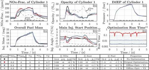This flexibility is demonstrated by the simulation results depicted in Figure 18. In contrast to Figure 17, $\mathrm{N}{\mathrm{O}}_{\mathrm{x}}$ has a lower priority compared to the fuel mass ($w_{\mathrm{N}{\mathrm{O}}_{\mathrm{x}}}=0.3,w_{\mathrm{F}}=0.7$). As the light blue case is trained only for the weight combination $w_{\mathrm{N}{\mathrm{O}}_{\mathrm{x}}}=w_{\mathrm{F}}=0.5$, its corrections strongly deviate from those of the online optimisation (red). However, the dark blue case, which is trained with the full range of the $\mathrm{N}{\mathrm{O}}_{\mathrm{x}}$ and fuel mass weights, adapts its predictions respectively and shows the same error level that was already discussed for Figure 17.

Figure 18. Test of the data-based correction models V1 and V2, see Figure 15, for a weight factor configuration that is not included in their training data. ¹⁾ Each approach also simulates the gas exchange phase once per cycle which requires $\approx 0.6\mathrm{s}$ in addition.

6. Conclusion and outlook

In order to improve the transient engine operation, combustion control schemes based on a cycle-by-cycle online optimisation require accurate while sufficiently simple optimisation models. Accordingly, this paper proposes methods to enhance their consistency and computational efficiency. Respective results are discussed based on an online optimisation scheme that contains a hybrid cylinder chamber description where the states and outputs are calculated by coupled physics-/data-based models. To consistently calibrate the data-based parts of this hybrid set-up, the proposed two-step training procedure defines a certain calibration order for the data-based models involved in the state space and output calculations. In detail, the cylinder pressure surrogate model is generated prior to those which predict the emissions and torque of the combustion phase. The additionally suggested test bench measurements further support the generation of the data-based models as the gathered data is tailored to their application in the combustion optimisation. However, in terms of the test bench measurements, further research can be spent in varying the intake manifold temperature in addition to the pressure and oxygen fraction to increase the diversity of the data.

To improve the computational efficiency of the optimisation-based control, time-intensive calculations are moved from the online optimisation scheme into the training data of the data-based models. Different concepts are proposed and compared in a simulation-based test environment. According to the results, projecting the IMEP constraint into the data-based models strongly reduces the computational effort without any loss of accuracy. A warm start strategy even further increases the speed of this approach. Concepts that determine the fuel injection parameter adaptations from purely data-based correction maps are even faster, since they are trained offline with given optimisation results and thus are free of any optimisation overhead during runtime. However, this speed-up is achieved at the expense of a loss of accuracy and lower flexibility, since changes in the emission limit maps or untrained weight values cannot be considered. As the previous results are determined in a simulation-based test environment, they also need to be implemented, tested, and verified in a real-world setup, i.e. in a rapid control prototyping system or in an engine control unit. Consequentially, this will require to improve the computational efficiency of the calculations for the gas exchange phase as well. Even if the changed host environment affects the total run time of the discussed approaches, the identified trends, however, are expected to persist.

Disclosure statement

No potential conflict of interest was reported by the author(s).

References

- World Energy Council, Global Transport Scenarios 2050, London: World Energy Council, 2011.
- U.S. Energy Information Administration, International Energy Outlook 2019, Washington, DC, USA: U.S. Energy Information Administration, 2019.
- F. Leach, G. Kalghatgi, R. Stone, and P. Miles, The scope for improving the efficiency and environmental impact of internal combustion engines, Transportation Eng. 1 (2020), pp. 100005. doi:10.1016/j.treng.2020.100005.
- European Union, Regulation (ec) 715/2007 of the European parliament and of the council of 20 June 2007, Official J. European Union L, 171, 1–16.
- European Union, Commission regulation (eu) 2018/1832 of 5 November 2018 amending directive 2007/46/ec of the European parliament and of the council, commission regulation (ec) no 692/2008 and commission regulation (eu) 2017/1151, Official J. European Union L, 301, 1–314.
- T. Shen, M. Kang, J. Gao, J. Zhang, and Y. Wu, Challenges and solutions in automotive powertrain systems, J. Control Decision 5 (1) (2018), pp. 61–93. doi:10.1080/23307706.2017.1399092.
- G.P. Merker and R. Teichmann (eds.), Grundlagen Verbrennungsmotoren: Funktionsweise und alternative Antriebssysteme Verbrennung, Messtechnik und Simulation, 8th ed., ATZ/MTZ-Fachbuch, Springer Vieweg, Wiesbaden, 2018.
- M. Wick, J. Bedei, D. Gordon, C. Wouters, B. Lehrheuer, E. Nuss, J. Andert, and C.R. Koch, In-cycle control for stabilization of Homogeneous Charge Compression Ignition combustion using direct water injection, Appl. Energy 240 (2019), pp. 1061–1074. doi:10.1016/j.apenergy.2019.01.086.
- S. Nakayama, T. Ibuki, H. Hosaki, and H. Tominaga, An application of model based combustion control to transient cycle-by-cycle diesel combustion, SAE International Journal of Engines 1 (2008), pp. 850–860.
- M. Grahn, K. Johansson, C. Vartia, and T. McKelvey, A Structure and Calibration Method for Data-driven Modeling of NOx and Soot Emissions from a Diesel Engine, Proceedings of the SAE 2012 World Congress & Exhibition, Detroit, Michigan, USA, 2012.
- R. Finesso, E. Spessa, Y. Yang, G. Conte, and G. Merlino, Neural-network Based Approach for Real-time Control of BMEP and MFB50 in a Euro 6 Diesel Engine, Proceedings of the 13th International Conference on Engines & Vehicles, Capri, Italy, 2017.
- M. Wick, J. Bedei, J. Andert, B. Lehrheuer, S. Pischinger, and E. Nuss, Dynamic measurement of HCCI combustion with self-learning of experimental space limitations, Appl. Energy 262 (2020), pp. 114364. doi:10.1016/j.apenergy.2019.114364.
- B. Berger, F. Rauscher, and B. Lohmann, Analysing Gaussian processes for stationary black-box combustion engine modelling, IFAC Proceedings 44 (2011), pp. 10633–10640.
- S. Hu, S. d’Ambrosio, R. Finesso, A. Manelli, M.R. Marzano, A. Mittica, L. Ventura, Y. Wang, and Y. Wang, Comparison of physics-based, semi-empirical and neural network-based models for model-based combustion control in a 3.0 l diesel engine, Energies 12 (18) (2019), pp. 3423. doi:10.3390/en12183423.
- M. Kang, K. Sata, and A. Matsunaga, Control-oriented cyclic modeling method for spark ignition engines, IFAC-PapersOnLine 51 (31) (2018), pp. 448–453. doi:10.1016/j.ifacol.2018.10.101.
- R. Finesso, O. Marello, E. Spessa, Y. Yang, and G. Hardy, Model-based control of BMEP and NOx emissions in a Euro VI 3.0l diesel engine, SAE International Journal of Engines 10 (2017), pp. 2288–2304.
- M. Grahn, K. Johansson, and T. McKelvey, A diesel engine management system strategy for transient engine operation, IFAC Proceedings 46 (2013), pp. 1–6.
- M. Mrosek, Model-based control of a turbocharged diesel engine with high- and low-pressure exhaust gas recirculation, Ph.D. diss., TU Darmstadt, 2017.
- S. Zydek, Optimale Regelung des Dieselmotors zur Minimierung von Realfahrtemissionen und -verbrauch, Ph.D. diss., TU Darmstadt, 2018.
- T. Makowicki, M. Bitzer, S. Grodde, and K. Graichen, Cycle-by-cycle optimization of the combustion during transient engine operation, IFAC-PapersOnLine 50 (1) (2017), pp. 11046–11051. doi:10.1016/j.ifacol.2017.08.2485.
- T. Makowicki, M. Bitzer, P. Kotman, and K. Graichen, A combustion cycle model for stationary and transient engine operation, IFAC-PapersOnLine 49 (11) (2016), pp. 469–475. doi:10.1016/j.ifacol.2016.08.069.
- R. Pischinger, Thermodynamik der Verbrennungskraftmaschine, 3rd ed., Springer Vienna, Vienna, 2009.
- J.B. Heywood, Internal Combustion Engine Fundamentals, McGraw-Hill, New York, USA, 1988.
- G.P. Merker, C. Schwarz, and R. Teichmann, Combustion Engines Development: Mixture Formation, Combustion, Emissions and Simulation, Heidelberg: Springer Science & Business Media, 2012.
- T.A. Henzinger, The theory of hybrid automata, Proceedings of the 11th Annual IEEE Symposium on Logic in Computer Science, New Brunswick, New Jersey, USA. 1996, pp. 278–292.
- R. S. Benson, The Thermodynamics and Gas Dynamics of Internal Combustion Engines, J. H. Horlock and D. E. Winterbone, eds., Oxford: Clarendon, 1986.
- F. Meddahi, C. Fleck, S. Grodde, A. Charlet, and Y. Chamaillard, Modeling waves in ICE Ducts: Comparison of 1D and low order models, Proceedings of the 12th International Conference on Engines & Vehicles, Capri, Napoli (Italy), 2015.
- P. Kotman, M. Bitzer, K. Graichen, and A. Kugi, Hybrid modeling of a two-stage turbocharged diesel engine air system, Proceedings of the 6th Vienna International Conference on Mathematical Modelling, Vienna (Austria). 2009, pp. 2015–2024.
- J. Warnatz, U. Maas, and R.W. Dibble, Combustion: Physical and Chemical Fundamentals, Modeling and Simulation, Experiments, Pollutant Formation, 4th ed., Springer, Berlin, 2006.
- K. Inagaki, M. Ueda, J. Mizuta, K. Nakakita, and S. Nakayama, Universal Diesel Engine Simulator (Unides): 1st Report: Phenomenological Multi-zone Pdf Model for Predicting the Transient Behavior of Diesel Engine Combustion, Proceedings of the SAE World Congress & Exhibition, Detroit, Michigan, USA, 2008.
- R. Finesso and E. Spessa, Real-time Predictive Modeling of Combustion and NOx Formation in Diesel Engines under Transient Conditions, Proceedings of the SAE 2012 World Congress & Exhibition, Detroit, Michigan, USA, 2012.
- H. Pitsch, H. Barths, and N. Peters, Three-dimensional modeling of NOx and soot formation in DI-Diesel engines using detailed chemistry based on the interactive flamelet approach, Proceedings of the SAE International Fall Fuels and Lubricants Meeting and Exhibition, San Antinio, Texas, USA, 1996.
- C.E.V. Rasmussen and C.K.I.V. Williams (eds.), Gaussian Processes for Machine Learning, MIT Press, Cambridge, Massachusetts, 2006.
- S. Angermaier and M. Gopalakrishnan, Implementation of data-based models using dedicated machine learning hardware (AMU) and its impact on function development and the calibration processes, Proceedings of the International Calibration Conference – Automotive Data Analytics, Methods and Design of Experiments (DoE), Berlin, 2017.
- ASCMO V5.5, ETAS GmbH, Stuttgart, Germany, 2020, Accessed 24 April 2021, Available at https://www.etas.com/de/portfolio/ascmo.php.
- L.V. Guzzella and C.H.V. Onder (eds.), Introduction to Modeling and Control of Internal Combustion Engine Systems, 2nd ed., Springer, Berlin, Heidelberg, 2010.
- D.V. Velmurugan, M. Grahn, and T. McKelvey, Diesel engine emission model transient cycle validation, IFAC-PapersOnLine 49 (11) (2016), pp. 1–7. doi:10.1016/j.ifacol.2016.08.001.
- K. Siebertz, D.V. Bebber, and T. Hochkirchen, Statistische Versuchsplanung: Design of Experiments (Doe), 2nd ed., VDI-Buch, Springer Vieweg, Berlin, Heidelberg, 2017.