
 ?Mathematical formulae have been encoded as MathML and are displayed in this HTML version using MathJax in order to improve their display. Uncheck the box to turn MathJax off. This feature requires Javascript. Click on a formula to zoom.
ABSTRACT
Percutaneous needle insertion constitutes a widely adopted technique for performing minimally invasive operations. Robot-assisted needle placement and virtual surgical training platforms have the potential to significantly improve the accuracy of these operations. For this, the development of mathematical models that provide a complete characterization of the underlying dynamics of medical needles is considered of paramount importance. In this paper, we develop two three-dimensional nonlinear rigid/flexible dynamic models of brachytherapy and local anaesthetic transperineal biopsy (LATP) needles. The proposed models relax the assumptions of previous investigations, quantify the vibrational behaviour and the rigid-body dynamics of medical needles and allow for real-time haptic and visual feedback information. Their accuracy and computational efficiency are assessed and validated using commercial software. The results show that, among the examined methods, the Rigid Finite Element Method provides the most accurate and numerically efficient solution for capturing the dynamics of flexible medical needles.
1. Introduction
In the last few decades, minimally invasive surgery (MIS) and localized therapy have become integral parts of modern medical practices as they offer significant advantages over conventional open surgery, such as decreased recovery time, lower risk of infection and reduced patient discomfort [Citation1]. One of the most widely used MIS procedures is percutaneous needle insertion, with a plethora of diagnostic and therapeutic applications, such as neurosurgery, deep brain stimulation, epidural anaesthesia, tissue biopsy and prostate brachytherapy [Citation2].
The success of the aforementioned operations is highly dependent on the accuracy of needle placement, while imprecise targeting often leads to severe complications, such as false negatives in biopsy or ablation of healthy tissue [Citation1]. However, accurate percutaneous needle placement is a highly challenging task. The limited visual feedback during the operation, combined with factors such as tissue anisotropy, heterogeneity and variability in anatomical structures among patients make navigation through tissue particularly complicated and decrease the procedure’s overall accuracy [Citation3].
In recent years, there has been significant effort to provide robust solutions for increasing the accuracy of needle placement procedures. Research has mainly focused on the development of robotic systems that allow autonomous or semi-autonomous navigation and accurate needle placement to targeted locations inside soft tissue [Citation4,Citation5]. Furthermore, the development of high-fidelity visual/haptic surgical simulators has allowed the training of junior surgeons in a variety of surgical scenarios and the preoperative planning of complex procedures by experienced doctors, leading to an overall improvement of the needle’s placement accuracy [Citation2,Citation6,Citation7].
A key requirement for the implementation of robotic guidance or simulated training solutions is the formulation of mathematical models that can accurately describe the dynamics of needle insertion. A common practice found in the literature is the division of the needle insertion modelling problem into three separate components [Citation8]: [a)] the modelling of the soft tissue [Citation9–11], the characterization of the interaction forces between the needle and the surrounding medium [Citation1,Citation12,Citation13] and the modelling of the flexible needle [Citation8,Citation14,Citation15]. This division allows the development of decoupled mathematical models for the needle and the tissue, while needle–tissue interaction is often modelled based on experimentally derived generalized force profiles at the needle’s base during needle insertion procedures [Citation1].
This work focuses on the formulation of accurate and computationally efficient models of flexible medical needles. These are of paramount importance as they not only provide an accurate description of the needle’s behaviour but also allow for the minimization of the stochasticity that is present during the aforementioned experimentally derived models of needle–tissue interaction. As a result, accurate needle models can significantly improve the identification accuracy of needle–tissue interaction dynamics, and, thus, constitute a key prerequisite for the systematic modelling of needle insertion procedures.
1.1. Related work
A complete characterization of flexible medical needles aims to identify the relationship between the spatio-temporal behaviour of the needle’s geometry and the specified motion trajectory at its base (e.g. insertion velocity, axial and lateral rotation), under the effect of some arbitrary loading conditions acting on its shaft. Furthermore, complete needle models provide information about the reaction forces at the needle’s base, due to the combined effect of the input driving constraints and the input loading conditions. The following paragraphs provide a review of various computational methods that have been developed to tackle some or all of these modelling requirements.
In the study by Webster et al. [Citation16], a novel non-holonomic model, based on a variation of the kinematic bicycle model, was proposed. The model allowed for a computationally efficient estimation of the needle’s deflection given the insertion and rotation speed of its base. However, the model did not provide any information about the vibrational behaviour of the needle and the profiles of the associated reaction forces. Furthermore, due to its various modelling assumptions, the method led to significant deviations when compared with experimental studies [Citation14]. Extensions of this model have been used in the literature for the development of kineto-dynamic path planning algorithms [Citation17,Citation18].
The need for more accurate needle models and information about the dynamic properties of needle insertion has led to a transition from kinematic to mechanics-based modelling approaches. Researchers [Citation15,Citation19,Citation20] developed quasi-static needle models, based on the linear Euler–Bernoulli beam theory, to describe needle deflection during percutaneous insertion procedures. While this modelling approach offered simplicity and computational efficiency, its linearity assumption led to invalid solutions when large deflections were considered [Citation8,Citation21]. To account for the geometric nonlinearity and minimize the targeting error of linear modelling approaches, DiMaio and Salcudean [Citation22] and Goksel et al. [Citation8] developed quasi-static methods based on nonlinear 2D and 3D Finite Element Method (FEM). Similarly, Adagolodjo et al. [Citation23] presented a geometrically nonlinear quasi-static model of flexible needles based on FEM and the co-rotational formulation. These models provided both computational efficiency and high accuracy when compared with experimental results for describing the steady-state responses of both large and small needle’s deflections.
Both linear and nonlinear models described above estimate needle’s deflection assuming a quasi-static needle insertion. In other words, it is assumed that the needle is inserted at a rate that does not allow for any oscillatory transients to occur and deflection is approximated by a sequence of steady-state responses. This assumption, however, does not provide any information about the vibrational behaviour of the needle and does not account for the correlation between its deflection and the system’s input parameters, such as its insertion velocity and the rate of axial rotation. This poses significant limitations as needle insertion is a highly dynamic procedure [Citation24]. As shown in the study by Podder et al. [Citation25,Citation26,], during brachytherapy operations, input parameters, such as the insertion velocity, span a wide range of values and considerably affect the needle’s deflection and vibration. More specifically, few studies [Citation20,Citation27–30] have proven the strong coupling of parameters such as the needle insertion speed, vibration and axial rotation to the needle–tissue interaction force and, subsequently, to its deflection. Furthermore, axial needle rotation and vibration can be used for minimizing needle deflection during needle insertion procedures [Citation20,Citation31–33]. Incorporation of such parameters naturally requires a dynamic model of flexible needles and not a quasi-static one. Therefore, accounting for the underlying needle dynamics is crucial for the complete characterization of needle insertion and, subsequently, for the development of accurate simulation solutions and precise control algorithms [Citation24].
Due to these limitations, it is necessary to develop modelling methodologies that incorporate the underlying needle dynamics. Khadem et al. [Citation14] proposed a novel dynamic model of a rigid/flexible 2D needle based on the Rayleigh-Ritz approximation technique and the linear Euler–Bernoulli beam theory. This work was one of the first to introduce the importance of dynamic modelling in needle insertion procedures, but it had significant limitations due to modelling assumptions, such as the beam’s linearity and unmodelled torsional dynamics. In the study by Martsopoulos et al. [Citation34], both the Rayleigh-Ritz and the FEM approaches were employed for capturing the three-dimensional dynamics of a rigid/flexible model of brachytherapy needles. However, the proposed models were based on infinitesimal strain theory and, thus, they did not account for geometric nonlinearities and large needle deflections. Similarly, Haddadi and Hashtrudi-Zaad [Citation24] extended the static angular spring FEM approach of Goksel et al. [Citation8]: the model captured the dynamics of needle insertion, while accounting for geometric nonlinearities due to large deflection, but it was only limited to 2D applications.
1.2. Contributions
Extending the work of Khadem et al. [Citation14,Citation24], Haddadi and Hashtrudi-Zaad [] and Martsopoulos et al. [Citation34], this paper develops and compares two different modelling approaches that aim to provide a complete characterization of the three-dimensional dynamics of flexible medical needles. For this, we employ the theory of flexible multibody dynamics (FMD), as it provides a plethora of computational tools that allow a systematic characterization of the needle’s spatio-temporal behaviour, under arbitrary driving constraints and loading conditions. The two formulations are examined based on three criteria: accuracy, computational efficiency and suitability to provide robust and stable solutions for the particular properties of the examined system (e.g. properties of numerical stiffness and shear locking due to the thinness of the needle are considered). The proposed methods are derived and solved using a systematic approach that allows direct comparisons to be performed. Special attention is paid to the computational efficiency of the methods, with the development of efficient solution strategies and numerical integration schemes, while concurrent execution and parallel programming concepts are also considered. Three simulation scenarios are developed and compared with commercial software solutions.
To the best of the authors’ knowledge, this is the first work to investigate and employ the theory of FMD for modelling the dynamics of flexible medical needles, and to provide a systematic comparison among different modelling techniques, while accounting for the challenges that are unique to needle insertion procedures. It is also the first to investigate both large rigid body motion of the needle’s base and large needle’s deflections and relax the modelling assumptions of previous research works (e.g. linearity assumptions, unmodelled dynamics, 2D models). Furthermore, to the best of the authors’ knowledge, this work is the first to apply the DDM and RFEM methods for modelling the dynamics of flexible needles. Even though approaches similar to the RFEM method have been used by Goksel et al. [Citation8] and Haddadi and Hashtrudi-Zaa [Citation24], there was no explicit reference to the RFEM. Instead, in both cases, the authors proposed the modelling of a flexible needle with a set of rigid bodies interconnected with angular springs. The meshing methodology of the RFEM was not taken into account, while the parameters of the angular springs were based on experimental data and not on the theory of continuum mechanics, as proposed by Wittbrodt et al. [Citation35]. Furthermore, contrary to the RFEM, the springs had only rotational and no translational degrees of freedom.
We believe that this work provides a well-rounded modelling approach without the need for any simplifications that compromise the overall accuracy of the system. Our aim is that the flexibility that this model provides will be used for finding further correlations between the movement of the needle’s base and the forces acting on it during its interaction with the soft tissue. Furthermore, we hope that the computational efficiency of this model will allow its integration with needle–tissue interaction models and the derivation of model-based control algorithms for automating needle insertion procedures.
1.3. Medical needles and flexible multibody dynamics
This section provides an overview of different FMD formulations and presents some essential considerations for choosing the appropriate approach for modelling the dynamics of flexible medical needles. Shabana [Citation36] a detailed review of available techniques of FMD systems theory is presented. The key difference between the methods lies in the selection of the generalized coordinates and the associated coordinate frames that are chosen to describe the system’s configuration. This allows the separation of the available formulations into two main categories: the local and the absolute frame approaches [Citation37].
In the local frame approaches, the deformation field of a flexible body is described with the help of nodal coordinates that are measured with respect to some local frame of reference, while its rigid body motion is defined based on the inertial description of the frame’s position and orientation. Some of the most widely used local frame approaches are the floating frame of reference (FFR), the convected coordinate system (CCS) and the large rotation vector (LRV) [Citation36]. As discussed by Shabana [Citation36], the CCS formulation results in inexact modelling of the rigid body dynamics of flexible structures, while the LRV formulation leads to numerical singularities and locking problems when analysing slender flexible bodies, such as the ones considered in this application.
In the majority of the research in the literature, the FFR formulation is combined with classical linear finite-element methodologies or other linear implementations of the assumed modes method, such as the Rayleigh-Ritz or the Galerkin’s methods. Even though these approaches allow the description of arbitrarily large rigid body motions, they are only valid when small deformations of the flexible components are considered [Citation38, pp. 309]. To address this, there have been various studies on the combination of the FFR formulation with the finite strain theory, to allow the analysis of geometric nonlinearities and large deflections [Citation39–43]. The nonlinearity is added to the system with the addition of the higher-order terms on the flexible body’s elastic potential energy. Even though this methodology allows the straightforward incorporation of the system’s geometric nonlinearity and a computationally efficient solution, it suffers from the numerical problem of element locking, as described by Reddy [Citation44]. While numerical remedies have been proposed to address this problem, such as the reduced-order Gaussian integration [Citation45, pp. 279–280], due to their heuristic nature, they introduce uncertainty to the problem and, thus, are not considered in our work.
To allow the description of both large rigid body motion and large deformation, a new set of methods, known as absolute frame approaches, were developed [Citation36]. Using these techniques, the pose and the deformation field of a flexible body is described using inertially defined nodal coordinates. The most widely used technique of this category is the absolute nodal coordinate formulation (ANCF), proposed by Shabana [Citation46]. For beam elements, the choice of nodal coordinates in ANCF relaxes the assumptions of Euler–Bernoulli and Timoshenko beam theories and allows large deflections and cross-sectional deformations to be considered [Citation47]. While the method requires a larger number of generalized coordinates and leads to highly nonlinear expressions for the system’s generalized elastic forces, it results in a constant mass matrix which significantly simplifies the associated equations of motion and accelerates computations [Citation48].
Whilst ANCF seems to meet the requirements of flexible needle modelling, as defined in Section 1, the method has reportedly led to significant numerical and convergence problems when dealing with thin and stiff structures, such as the ones considered in our work [Citation49–51]. This phenomenon, known as Poisson locking, stems from the coupling between the high-frequency cross-sectional deformation modes (found in thin and stiff elements) and the other deformations (e.g. axial and bending) [Citation49]. To address this, different approaches have been proposed in the literature, such as the development of higher-order thin elements [Citation52], the uncoupling between the shear deformation and antisymmetric bending [Citation50] and the redefinition of the system’s degrees of freedom (DOFs) [Citation53]. While some of the proposed techniques have the potential to alleviate the problem of Poisson locking, they introduce additional modelling complexity [Citation50] or remove the initial benefits of the ANCF, such as the formulations of Gruber et al. [Citation53] and von Dombrowski [Citation54] that lead to a non-constant mass matrix.
As an alternative to the ANCF, our work proposes the modelling of flexible needles with the use of the discrete deformation mode (DDM) formulation, presented by Jonker and Meijaard [Citation55]. A comparative analysis between DDM and a modified (locking-free) version of ANCF in the study by Schwab and Meijaard [Citation50] shows that the DDM (which also belongs to the family of the absolute frame approaches) allows for an accurate and computationally efficient description of large reference motion and deformation of thin flexible elements without introducing further modelling complexity. Furthermore, we also propose the modelling of flexible medical needles with the help of the rigid finite element method (RFEM). This technique, which also belongs to the absolute frame approaches, is well suited for the current application, as it has successfully been applied for capturing the nonlinear dynamics of slender structures [Citation56,Citation57] without leading to the aforementioned numerical problems.
The importance of modelling both large rigid body motion and large needle deformation for prostate biopsy and brachytherapy procedures can be clarified with the help of . In these procedures, and especially LATP biopsies that use a precision point transperineal access system [Citation58], the surgeon’s hand performs large rigid body motions in order to guide the needle in the desired location. As illustrated in , this can cause significant overall needle deflections, while needle deflections inside the tissue could still remain small.
Figure 1. Large deflections and large rigid body motion in prostate brachytherapy and biopsy.
As a result, it is crucial to provide a mathematical model that captures both large rigid body motion and large needle deflections. The reason for this is twofold:
• One of the possible applications of a high-fidelity needle model is the development of haptic simulators for training junior surgeons in LATP biopsies. It is, thus, important to provide a mathematical model that captures the dynamics of the needle insertion in its entirety without introducing any limiting assumptions. This would give trainees the ability to test even the ‘extreme’ regions of their input space as they would do in a real training environment.
• A highly accurate dynamic model of needle insertion can provide insights into the identification of needle–tissue interaction forces, as it captures the correlations between the needle’s state (deflection) and the imposed trajectory at its base. Introduction of modelling assumptions, such as the quasi-static needle insertion or small needle deflections, does not allow the investigation of these correlations, as they restrict the system’s input and state space. Thus, to understand the real dynamics of needle insertion procedures, it is critical to remove these assumptions and investigate the true correlation between input (imposed trajectory) and output (deflection/forces). By improving our understanding of these correlations, there is the potential to build improved algorithms for robot-assisted needle insertion procedures (e.g. by building better model-based control algorithms).
1.4. Needle–tissue interaction
This section analyses existing needle–tissue interaction models and formulations. As discussed by Rossa and Tavakoli [Citation59], during needle insertion the deformed needle shaft compresses the surrounding tissue which, in turn, applies forces to the former influencing its deflection. As a result, needle deflection and tissue deformation are coupled effects that influence each other [Citation59].
There are two main approaches for identifying these interactions, which, in this work, are referred to as constrained and unconstrained approaches. In the constrained approach, the needle and tissue are studied as a unified system. Needle–tissue interactions are imposed as kinematic constraints between the two mediums, and the system’s equations for both the needle and tissue are solved simultaneously [Citation22,Citation60,Citation61]. The reaction forces between the two bodies are then obtained with the help of LaGrange multipliers. However, this approach presents some shortcomings. First, in cases where the tissue is modelled with the help of FEM, this technique requires that the tissue mesh is adapted at each time step to match the discretization of the needle and allow the enforcement of the kinematic constraints on the corresponding nodes of the tissue and the ones of the needle [Citation22]. The computational cost of this remeshing makes the application of this technique unsuitable for interactive applications. One possible solution is using a meshless discretization, as in the study by Xu et al. [Citation62], or using the technique of local constraints presented by Wang and Hirai [Citation63]. Second, the model requires knowledge of the exact mechanical properties of the tissue on its interface with the needle. However, monitoring the medium’s properties on this interface is not usually plausible or applicable in real-time applications or in vivo tests [Citation64]. Finally, coupling the two flexible mediums leads to a high-dimensional set of equations that is challenging to solve in real-time.
In the unconstrained approach, the needle–tissue interaction is modelled with the help of interface force models. These forces, which are functions of both the needle’s and tissue’s state, are imposed simultaneously but separately on the tissue and the needle, allowing the mathematical decoupling of the two. Furthermore, these models are dependent on a small number of parameters. The unconstrained modelling method is quite popular as it is both simple and computationally efficient, allowing its application to interactive surgery simulation and control. However, it suffers from limited accuracy as the identification of these force profiles is usually based on semi-empirical approaches and experimental observations. A plausible remedy to this is the use of online system identification algorithms for the tuning the model’s parameters [Citation65].
One of the most widely used unconstrained models is the one proposed by Okamura et al. [Citation1]. Experimental studies reported in the study Okamura et al. [Citation1] showed that the axial forces acting on the needle’s base are the summation of stiffness, friction and cutting forces. These forces depend on the relative state (position and velocity) of the tissue and the needle and are distributed along the needle’s shaft. Since the work of Okamura et al. [Citation1], significant research has been devoted to the definition of mathematical models that can accurately capture these force profiles. For example, whilst Okamura et al. [Citation1] proposed a modified Karnopp friction model, different friction modelling approaches were then adopted by Asadian et al. [Citation66] and Yang et al. [Citation67]. Similar, simplified interaction force models have been developed for modelling the distributed lateral loads acting on the needle’s shaft as is inserted inside the tissue. The most popular approach is modelling the lateral tissue forces as virtual springs (both linear and nonlinear) of varying mechanical properties, similar to the Winkler foundation model [Citation19,Citation68–70].
This section provided an overview of existing modelling approaches in needle–tissue interaction. In Section 2, we develop mathematical needle models based on two formulations [a)] the DDM (Section 2.1) and the RFEM (Section 2.2). A simulation algorithm for obtaining the needle’s state is analysed in Section 2.3 while needle–tissue interaction models are formulated in Section 2.4. Real-time considerations are discussed in Section 2.5. Section 3 presents the results from three different simulation scenarios, the interpretation of which is provided in Section 4. Concluding remarks are given in Section 5.
2. Materials and methods
In this work, we focus on moderately flexible medical needles, such as those used in prostate brachytherapy and local anaesthetic transperineal prostate (LATP) biopsy, shown in . We propose a model, shown in , that considers a) the base of the needle as a rigid body that follows any arbitrary spatial trajectory, imposed by a surgeon or a robotic arm, and the shaft of the needle as a flexible body that is rigidly attached to the base and deforms elastically under a general state/time-dependent field of forces, which corresponds to the interactions between the needle and the surrounding tissue.
Figure 2. Brachytherapy/LATP needle model.
To describe the motion of the system shown in , we introduce the following frames of reference: let be the inertial frame of reference and
a frame rigidly attached to the rigid body’s centre of mass
. Furthermore, we introduce a floating frame of reference (FFR)
which is rigidly attached to point
of the rigid body. As shown in , the orientation of the frames
and
is identical and fixed, i.e. there is no relative motion between them.
In the following formulations, the needle is considered as a slender and homogeneous beam with circular cross-section and constant mechanical and geometrical properties along its span. The material of the needle is isotropic and linear. Furthermore, we introduce the notation which describes the position of a vector
with respect to frame
expressed in frame
[Citation71, pp. 13–16]. The following sections present the kinematic and dynamic description of the aforementioned needle model based on the two proposed FMD formulations, namely, the DDM and the RFEM approaches. In both approaches, we first introduce the kinematic description of the model and then derive expressions for the virtual works of the forces acting on the structure. Next, using D’Alembert’s form of the principle of virtual work, we express the dynamic equilibrium of the system and derive the equations of motions. These steps are thoroughly presented in Sections 2.1 and 2.2.
2.1. Equations of motion: DDM approach
2.1.1. Kinematic description
The DDM method employs a spatial discretization of the needle’s geometry into beam elements, each of which is described using inertially measured nodal coordinates. More specifically, as shown in complete characterization of the configuration of the beam element
can be acquired based on the inertially measured cross-sectional position and orientation at its nodes
and
, while intermediate points are defined with the help of interpolation functions. The element’s vector of generalized coordinates can be defined as
Figure 3. Spatial DDM element at reference and deformed state.
where and
are the inertial positions of the nodal cross-sections’ midpoints
and
, while
and
are the Euler angles, based on the sequence of intrinsic rotations
-
-
, that define the cross-sectional orientation at nodes
and
. These are defined as
With the help of the Euler angles and
, the set of triad unit vectors, shown in , are defined as
The rotation matrices and
describe the orientation of the local frames
and
with respect to the inertial frame of reference
. The
and
are constant unit vectors pointing in the associated directions
and
. The inertial position of point
of element
, illustrated in , can be obtained with the help of the generalized element coordinates and interpolation functions
as
Expressions for the , can be chosen as in the study by Jonker and Meijaard [Citation55], while the scalar
is the point’s distance along the element’s elastic line measured using the co-rotational frame introduced by Jonker and Meijaard [Citation55]. Based on Equationequation (2)
(2)
(2) , the inertial velocity of point
can be expressed as
where
The matrices and
in the above expression map the derivatives of the Euler angles
and
to the respective frame rotational velocities, such that
Based on Equationequation (3)(3)
(3) the inertial virtual displacement of point
is given as
while the acceleration of point takes the form
In the above expression, the Coriolis/centrifugal component of acceleration is given as
where
Similarly, the orientation of the cross-sections along the element’s length can be written as
where expressions for the interpolation vector functions ,
and
can be found in the study by Schwab and Meijaard [Citation50]. If the mapping from the nodal components of the Euler angles to the generalized element’s coordinates is defined as
, with
, then the above expressions take the form
2.1.2. Virtual work
Next, we derive the virtual work of the inertial forces of element . To simplify the associated expressions, it is assumed that the inertial forces caused by the transversal shear deformation of the element’s cross-section are negligible due to the needle’s thickness. Based on this assumption, the virtual work of the inertial forces of element
can be defined as
where is the mass,
the length,
the polar moment of area and
the density of element
. The second term of the above equations employs the first component of the sequence of Euler angles
to describe the inertial forces due to the element’s torsional dynamics. Using Equationequations (4)
(4)
(4) , (Equation5
(5)
(5) ) and (Equation6
(6)
(6) ), the above expression can be rewritten as
where . The mass matrices
and
are defined as
The generalized Coriolis/centrifugal vector takes the form
The key component of the DDM method is the deformation modes, which provide a complete characterization of the beam element’s deformation field. These modes can be specified using six independent generalized strain expressions, which are functions of the element’s inertially defined generalized coordinates [Citation72]. The generalized strains, which remain invariant under arbitrary rigid body motions and orthogonal coordinate transformations [Citation72], take the form
where and
. In Equationequation (8)
(8)
(8) , the generalized strain
is used to describe the beam’s axial elongation,
is for torsion, while
describe transversal bending. To account for geometric nonlinearities, second-order terms can be added in (8). The modified second-order generalized strains can be calculated as
where expressions for the function , which incorporates the second-order terms, and the function
, which maps the generalized coordinates to generalized strain measures, are given by Jonker and Meijaard [Citation55]. Furthermore, if it is assumed that the beam has been divided into a sufficient number of elements so that the strains remain small, then the generalized strains can be associated with the generalized stresses (Voigt notation) using the constitutive law written as [Citation50]
where is the element’s constant symmetric stiffness matrix, defined by Schwab and Meijaard [Citation50]. Based on Equationequation (9)
(9)
(9) , the infinitesimal change of the generalized strains can be calculated as
With the help of Equationequations (9)(9)
(9) , (Equation10
(10)
(10) ) and (Equation11
(11)
(11) ), the virtual work of the element’s elastic forces can be written as
Similarly, the virtual work of the element’s damping forces can be written as , where the generalized damping forces
can be modelled using various approaches, as discussed by Yoo et al. [Citation73].
Next, we define the virtual work for the external forces. For this, it is assumed that a random point of element
, located at the beam’s elastic line and at a distance
from the nodal point
, is subjected to a point force
and a point moment
, shown in .
Figure 4. Free body diagrams for DDM and RFEM methods.
Then, the virtual work resulting from these forces and moments can be written as
Using Equationequations (4)(4)
(4) and (Equation6
(6)
(6) ), the above expression takes the form
where and
. The virtual work of the external generalized forces presented in Equationequation (13)
(13)
(13) can be extended to accommodate for
point forces and
point moments. In this case, it can be proven that the total virtual work of the external generalized forces is given as
Finally, the virtual work of the external generalized constraint forces for element can be calculated as
.
2.1.3. Dynamic equilibrium
To derive the flexible needle’s equations of motion we apply the dynamic equilibrium expression based on D’Alembert’s form of the principle of virtual work, which can be written as
The virtual works of the above expression can be calculated considering the contributions from the individual elements as
Substituting the derived virtual work expressions, the above equation becomes
If we introduce the mapping from the local generalized coordinates of element
to the flexible beam global generalized coordinates
, such that
, then the above expression can be written as
with
Due to the explicit integration of the constraint forces in the above expression, the generalized coordinates of the flexible body can be treated as independent and, thus, its equations of motion can be expressed as
2.2. Equations of motion: RFEM approach
2.2.1. Kinematic description
The main idea of the RFEM method is replacing flexible bodies with a system of rigid finite elements (rfes) that are interconnected via spatial spring-damping elements (sdes) [35, pp. 35]. The first step towards describing the kinematics of the proposed method is the division of the flexible body into rfes and sdes. This division can be performed in two stages [35, pp. 37–40]. First, the flexible body is divided into elements, each of which has a length
, where
is the needle’s total length. The sdes are added at the centre point of the initial elements, as shown in . In the secondary division, the initial elements are divided again, so that their edge points are interconnected by the sdes. As shown in , intermediate rfes have now length equal to
, while the first and last rfe have a length of
. The configuration of the flexible body can now be described with the help of the resulting
rfes. For this, we consider the rfe
shown in . Due to the rigidity assumption, the configuration of the rfe
can be completely characterized with the help of the body frame
, which is rigidly attached to the element’s centre of mass
shown in . More specifically, the inertial position of an arbitrary point
of element
is given as
Figure 5. Needle division to rfes and sdes.
Figure 6. Spatial RFEM element.
where is the origin of frame
measured in the inertial frame
and
the rotation matrix that describes the orientation of frame
with respect to
. As before, the rotation matrix is parameterized using the set of Euler angles
that describe the sequence of intrinsic rotations
-
-
. It should be noted that, due to the rigidity assumption and contrary to the DDM method, the distance
is constant. Thus, a complete characterization of the rfe
configuration can be obtained using the generalized coordinates
Based on expression (18), the inertial velocity of point is given as
The matrix maps the derivatives of the Euler angles
to the rotational velocity of frame
, such that
Similarly, the inertial acceleration of point can be defined as
where
Furthermore, based on Equationequations (18)(18)
(18) and (Equation20
(20)
(20) ), the inertial virtual displacement of point
can be written as
2.2.2. Virtual work
Similarly to Section 2.1.2, the virtual work of the inertial forces can be defined as
which, using Equationequations (21)(21)
(21) and (Equation22
(22)
(22) ), leads to
with
and
The key component of the RFEM is the definition of the elastic forces that act on each rfe. As shown in , the rfe is subject to the elastic forces
and the elastic moments
due to the deformation of the associated sdes
and
. Based on , these forces and moments can be modelled as [Citation56]
Figure 7. Elastic forces in RFEM.
The indices and
refer to spring and damping forces/moments, respectively. These can be modelled as
with and
the
null matrix. Expressions for the constant stiffness and damping matrices
and
can be found in [35, pp. 69–82]. In the above expression, vectors
and
denote the translational deformation of the sdes
and
respectively, and can be written as
Similarly, the elastic moments in Equationequation (24)(24)
(24) are modelled based on the rotational deformations of the associated sdes
and
, denoted as
and
. Due to the non-commutative property of Euler angles, these can be extracted from the rotation matrices
and
accordingly. From the expression above, the element’s generalized elastic forces are nonlinear functions of the system’s generalized coordinates. As a result, if these expressions are treated as forces external to the element
, then the virtual work caused by the generalized elastic and damping forces can be written as
where
and
The locator matrix in the above expression maps the element’s Euler angles to the element’s generalized coordinates such that
.
Next, the virtual work of the external forces is defined. For this, we consider the point of element
, located at the position defined by the vector
with respect to frame
, which is subject to the point force and point moment pair illustrated in . Then, as illustrated in Section 2.1.2, the virtual work resulting from these forces and moments can be written as
Using Equationequation (22)(22)
(22) and the matrix
, the above expression can be written as
where . If we consider that the element
is subject to
point forces and
point moments, it can be shown that the total virtual work of the external generalized forces is given as
2.2.3. Dynamic equilibrium
The procedure for deriving the equations of motion for the flexible beam is identical to the one presented in Section 2.1.3. First, we define the mapping from element’s local generalized coordinates
to the beam’s global generalized coordinates
as
. Then, following the steps of Section 2.1.3, it can be shown that the equations of motion of the flexible beam using the RFEM method take the form
where the mass matrix and the generalized force vectors can be calculated as in (16).
2.3. Simulation algorithm
As illustrated in the previous sections, the two proposed approaches lead to the same set of equations, given in (17) and (28). This allows the development of a common solution strategy, independent of the method used, as well as the implementation of direct comparisons between them. To provide a more compact form of the above equations we define the vector
Then, Equationequations (17)(17)
(17) and (Equation28
(28)
(28) ) can be rewritten as
As stated in Section 1, the aim of the solution algorithm is to provide an accurate and computationally efficient description of the needle’s three-dimensional dynamics, as the rigid base’s centre of mass follows an arbitrary trajectory imposed by the surgeon’s hand or a robotic gripper (driving constraints). Furthermore, the solution algorithm should describe the profiles of the reaction forces
and moments
, illustrated in , that result from the combined effect of the structure’s rigid body motion and vibration. The following sections provide a detailed description of the process for deriving the required solution.
Figure 8. Rigid base and flexible needle at connection point .
2.3.1. Boundary conditions
Before the proposed algorithm is formulated, some important remarks for Equationequation (29)(29)
(29) must be made. More specifically, it should be noted that the state vector
contains the boundary conditions, due to the rigid connection between the flexible needle and the rigid base, as shown in . To eliminate the boundary conditions, the state vector
can be partitioned in the constrained
and active
coordinates such that
The constrained vector incorporates the prescribed motion of the associated coordinates (boundary conditions), while the active vector
describes the free (independent) coordinates that define the beam’s motion. Depending on the chosen FMD technique and according to the different sets of generalized coordinates defined in (1) and (19), the constrained vector
can take one of the following forms:
If and
are known functions, with continuous second derivatives, that describe the position and orientation of frame
(pose of surgeon’s hand or robotic gripper) with respect to the inertial frame of reference
, then, from the above expression and according to , it follows that the constrained vector
is also a known vector function. Furthermore, it follows that the linear and rotational velocity and acceleration of the constrained coordinates can be obtained.
2.3.2. Recursive Newton–Euler method
A widely used approach for solving the Equationequations (29)(29)
(29) while simultaneously obtaining the generalized reaction forces
and moments
profiles is the explicit incorporation of the system’s kinematic constraints through the use of the LaGrange multipliers [Citation74, pp. 323–349]. While this technique has been widely employed in the FMD literature for solving systems of interconnected bodies, it leads to a higher-dimensional system of coupled differential and algebraic equations, the solution of which requires special numerical treatment that increases the computational complexity.
Taking advantage of the specific properties of the needle insertion application, our work presents an alternative approach that can accelerate the solution of (29), while obtaining the required generalized reaction force profiles. More specifically, as the examined system is only under two sets of kinematic constraints, i.e. [a)] the connection of the flexible needle to the rigid base at point () and the driving constraints at the base’s centre of mass C, it allows the efficient implementation of the generalized recursive Newton–Euler method [Citation75], which can lead to accelerated solutions for a low number of kinematic constraints.
To implement the proposed algorithm, the equations of motion (29), based on the partitioning of (30), can be rewritten as
where
Note, the components of the vector are all known, except for the generalized constrained forces
. The key idea for obtaining the system’s solution is that the components of the constraint forces corresponding to the active system’s coordinates are zero,
. On the other hand, the components
, which result from the reaction forces due to the boundary conditions at point
, are finite and incorporate information about the connection forces
and moments
(). Based on this observation, Equationequation (31)
(31)
(31) can be written as
As the right-hand side of the above equation is known, the equation can be integrated numerically to identify the time evolution of the generalized active coordinates . Given that both the constrained and active coordinates are now known, the constrained components of the reaction forces are calculated for the current time step as
Based on the above equation, the reaction forces and moments
can be calculated with the help of the equations of motion of the rigid base. These can be written as
where is the rigid body’s mass,
its inertial tensor defined in the frame
and vector
the rotational acceleration of frame
or
, with respect to the inertial frame of reference. From the above equations and , the generalized reaction forces that act on the needle’s base are
and
The connection forces and moments
in the above expression are derived based on generalized constraint forces of (32).
2.4. Needle–tissue interaction forces
As discussed in Section 1.4, needle–tissue interaction is modelled with either constrained methods, by imposing kinematic constraints between the needle and its surrounding medium, or with unconstrained methods, through the development of needle–tissue interaction force models. Our work is independent of the needle–tissue modelling approach and can be combined with either the constrained or the unconstrained method. However, as discussed in Section 1.4, the constrained approach is highly dependent on the tissue modelling and discretization. Thus, to maintain the general nature of the proposed needle model, we will only study the unconstrained approach. Furthermore, we will only focus on the RFEM formulation, but a similar approach can be used for the DDM method.
First, we consider the last RFEM element , illustrated in , which incorporates the needle’s bevel tip. Based on the same figure, we define the needle’s tip point
as
Figure 9. Last RFEM element and needle tip definition.
with the element’s length and
the needle’s radius. Similarly, the position of the needle’s tip surface centroid
can be defined with the help of similar triangles as
As discussed in Section 1.4, the axial forces acting on the needle can be decomposed as a summation of a cutting/stiffness force acting on the needle’s tip and a friction force distributed along the needle’s shaft. The stiffness forces are due to the elastic properties of the tissue and occur right before the tissue/capsule puncture. On the other hand, friction and cutting forces occur after the puncture event.
In our work, both cutting and stiffness forces are modelled as point loads acting on the needle’s tip. We assume that the stiffness force is applied at the needle’s tip point and it remains parallel to the element’s local axis
, as shown in . The cutting force is assumed to be normal to the needle’s bevel surface and is applied at its centroid
[Citation68], as illustrated in .
Figure 10. Stiffness and cutting forces on the last RFEM element.
From the above figures, we can define the stiffness and cutting
forces expressed in the local element frame
as
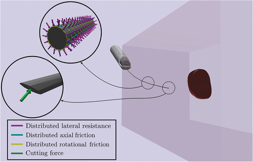
Friction forces are distributed along the needle’s shaft as it slides inside the tissue post-puncture. During the needle insertion, the needle’s shaft is also under the influence of distributed lateral forces due to the tissue compression. Both friction and lateral forces, illustrated in , can be considered as traction vectors acting on the needle’s surface and can be analysed with the help the needle’s tangent plane.
Figure 11. Illustration of post-puncture needle–tissue interaction forces.
More specifically, we first consider the rfe , shown in . Furthermore, we consider an arbitrary point
that belongs to the surface of the rfe
. The position of the point with respect to the element’s local frame
can be expressed with the help of cylindrical coordinates as
Figure 12. Infinitesimal area and tangent plane vectors for rfe .
where is the distance of the point
along the
axis of element
, illustrated in ,
is the radius of the needle (or that of the element rfe
) and
is the complementary polar angle illustrated in the same Figure.
EquationEquation (34)(34)
(34) is the parametric equation of the surface
of the element
. The surface is a function of two parameters, namely, the longitudinal distance
and the angle
. Using this parametric equation we can define the tangents and normals of the surface. More specifically, the unit vectors
and
at the point
shown in are defined as:
The unit vector at the point
is defined as
Note that vectors ,
and
are defined with respect to the element
frame
. Finally, observing , we can define the infinitesimal surface
as
To model the traction acting on the needle’s surface, we examine the rfe shown in . First, we assume that a mean traction vector
acts on the point
and it is transmitted across an infinitesimal area
. As shown in , this traction vector can be divided into three components, each of which points in the directions defined by the tangent and normal vectors
,
and
.
Figure 13. Traction on an infinitesimal area of rfe .
These components represent the distributed contact forces between the needle and the tissue as a result of their relative motion. More specifically, the traction represents the axial friction due to the longitudinal motion of the element, the traction
represents the rotational friction due to the needle’s axial rotation and the traction
represents the lateral resistance due to tissue displacement/compression. Based on and the definition of the tangent and normal surface vectors of element
, we can define the mean traction vector
transmitted across the infinitesimal area
as
The definition of the mean traction vector transmitted across the infinitesimal area allows the calculation of the total surface force acting on the element
. This is given by integrating over the entire surface
of the element
where and
are the lower and upper integration limits for the longitudinal distance of the element
. These values depend on the percentage of the element that is in contact with the tissue. Combining Equationequations (35)
(35)
(35) and (Equation36
(36)
(36) ) the total surface force on element
is given as
with
and
EquationEquations (33)(33)
(33) , (Equation37
(37)
(37) ), (Equation38
(38)
(38) ) and (Equation39
(39)
(39) ) can provide a full characterization of the needle–tissue interaction. These can be included in the RFEM needle model, using Equationequation (27)
(27)
(27) . To provide a complete characterization, however, it is essential to define expressions for the functions of stiffness, cutting, axial friction, rotational friction and lateral compression forces.
As discussed in Section 1.4, there is no unique modelling approach for characterizing these forces. For example, in the study by Okamura et al. [Citation1], cutting forces were modelled as constant, while Elgezua et al. [Citation76] proposed a quadratic cutting force model. Similarly, there are various formulations for the distributed loads. For example, friction forces in the study by Okamura et al. [Citation1] were assumed to be uniformly defined over the needle’s length () with a magnitude characterized by the modified Karnopp model. Other models, such as the LuGre friction model, have also been proposed [Citation66]. Applying a uniformly distributed Karnopp model for the friction forces of the element
in (37) leads to
with defined by Okamura et al. [Citation1]. A similar expression can be derived for the rotational friction and lateral tissue resistance of Equationequations (39)
(39)
(39) and (Equation38
(38)
(38) ). For complex distributed load expressions, the surface traction integrals can be computed numerically (e.g. through Gaussian quadrature) and applied as equivalent point loads on the RFEM elements.
This Section provided some guidelines regarding the integration of the proposed needle model with unconstrained needle–tissue interaction forces. However, characterizing the needle–tissue interaction forces is beyond the scope of this work. This preserves the general nature of our work and allows the reader to develop and integrate their own needle–tissue interaction models.
2.5. Real-time considerations
As discussed in Section 1, one of the key aims of our work is to provide both highly accurate and computationally efficient mathematical models that allow real-time execution. In this regard, except for the solution strategy presented above, which has been tailored to the requirements of the application to maximize computational efficiency, our work considers three more modelling and implementation aspects that contribute to the acceleration of the overall system’s performance.
The first strategy takes advantage of the structure’s geometry to decrease the computational complexity of the solution. More specifically, our work only considers beam finite elements for modelling the dynamics of flexible medical needles. The reason for this is twofold. First, beam elements have been specifically designed to tackle the particularities of beam-like structures, such as a biopsy needle and, thus, are expected to have superior performance when compared to generic finite elements, such as tetrahedrals or hexahedrals [Citation8]. Second, while 3D beam elements and tetrahedral elements might have the same number of nodal coordinates, tetrahedral-based meshes require the use of a significantly higher number of elements for covering the needle’s geometry. Furthermore, the requirement for mesh symmetry leads to a further increase in the number of required tetrahedral elements, while the employed beam elements are inherently symmetric [Citation8]. Thus, by considering only beam elements, our work aims to minimize the required computational complexity and accelerate the model’s solution.
The second strategy aims to tackle the numerical particularities of the problem. More specifically, due to the thinness of the examined structure, the needle’s axial and torsional stiffness is significantly higher than that in the transversal directions. This leads to a high ratio in the eigenvalues of the Jacobian of the vector function
in Equationequation (29)
(29)
(29) and, subsequently, to a significant deviation between the response time scales of the
vector components. This phenomenon, known as differential equation stiffness, creates significant numerical problems and needs special treatment.
In our work, different approaches have been considered for tackling the stiffness of the differential Equationequations (29(29)
(29) ), while allowing real-time execution. This includes the analysis of explicit, implicit, semi-implicit and multistep numerical integration approaches. Explicit integration techniques are not suitable for stiff differential equations as they lead to solution instability, unless an extremely small integration step size is chosen (which significantly increases the computational time) [Citation77]. On the other hand, implicit integration techniques can guarantee stability without the need for extremely small step sizes, at the cost of solving a set of nonlinear algebraic equations at each time step. To cover the numerical requirements of all of the proposed methods, our work employs diagonally implicit Runge-Kutta methods with an inner Newton-Raphson algorithm parallelized in multiple processing cores for improved performance. This technique leads to stable solutions and real-time execution. As will be discussed in Section 4, the numerical properties of the RFEM method also allowed the use of Rosenbrock-Type methods (or linearly implicit Runge-Kutta methods) [Citation77] leading to accuracy, stability and even further computational efficiency.
The third strategy stems from the concurrency that characterizes the proposed algorithms. More specifically, both the DDM and the RFEM methods include concurrent components that can be executed in parallel allowing for a significant improvement in the overall computational efficiency. Examples of these components are the generalized forces and mass properties that can be calculated independently among the different elements. By exposing the concurrency of the proposed algorithms and employing multithreading execution techniques, the integration time of EquationEq. (29)(29)
(29) was significantly accelerated.
3. Results
To demonstrate the performance of the proposed algorithms, three numerical examples are presented in this section. These were designed to give insight into the accuracy and computational efficiency of the proposed methods for both the static and dynamic analysis of the system, while aspects of linear and nonlinear deflection were also considered.
For the validation of the proposed methods, the simulation scenarios were also solved with the help of commercial simulation software. More specifically, the Ansys software was used for the static analysis of the needle’s deflection, while dynamic simulations were performed with the help of MSC Adams. The simulations were implemented on a 4-core Intel® Core™ i7-7700HQ CPU running at 2.80 GHz, using the C++ Armadillo library [Citation78] with the Intel Math Kernel Library (MKL) integration. Aspects of algorithmic parallelization were implemented with the help of the OpenMP API [Citation79].
The needle’s base was treated as a solid cylinder with length = 0.153 m, radius
= 0.017 m and a mass of
= 0.09 kg. The flexible needle was modelled as a homogeneous stainless steel beam with a circular cross-section of radius
and a length of
. Both the mechanical and geometrical properties of the needle were assumed to remain constant along its span. The properties of the system were based on commercially available bevelled tip LATP needles. Next, the three numerical examples are presented.
3.1. Steady-state analysis: tip force loading
First, we examine the steady-state deflection of the flexible needle, using the two proposed FMD approaches. The needle’s deflection results from a constant point force loading applied at its tip (point B, ). To analyse the performance of the proposed techniques, we consider three spatial loading conditions:
The gradual increment in the loading allows the analysis of the effect of the large needle deflection on the accuracy of the proposed methods. To examine the accuracy of the methods, the problem is also solved using Ansys (both linear and nonlinear solver). shows the transversal and
deflection for the three tip force loading conditions
,
and
of (40). shows the error measure
Figure 14. Needle response under the three tip force loading conditions of (40).
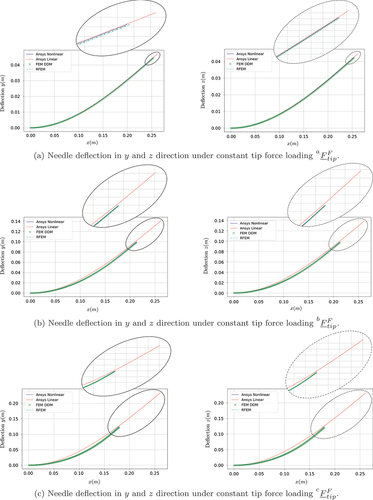
Figure 15. Error under the three tip force loading conditions of (40).
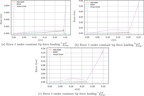
where and
correspond to the deflections calculated from the Ansys nonlinear solver.
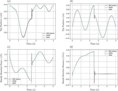
3.2. Transient analysis: step force loading and sinusoidal base movement
Next, we examine the dynamic behaviour of the flexible needle. For this simulation scenario, the needle’s rigid base undergoes a sinusoidal motion, while a step force loading is applied at its tip. More specifically, the input driving constraint has the form
where . The excitation magnitude
and frequency
were arbitrarily chosen as
and
. The external force vector, applied at the needle’s tip B, is chosen as
The magnitude has a value of
, while
is the Heaviside function. For the simulation results shown in ), a spatial discretization of four elements is chosen for both methods. The system’s solution using the MSC Adams software acts as a reference point for testing the accuracy of the proposed approaches.
Figure 16. (a) Response of tip’s position in direction. (b) Response of tip’s position in
direction. (c) Reaction force at needle’s handle in
direction. (d) Reaction moment at needle’s handle in
direction.
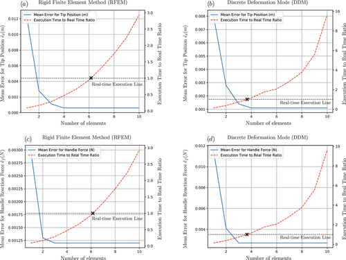
To analyse the convergence, accuracy and computational efficiency of the two methods, the following error metrics and ratios are introduced. First, the error metrics that define the time-averaged deviation of the tip position and the reaction force
from the MSC Adams results are defined as
and
where is the number of points used for the temporal discretization,
and
. Next, the computational efficiency of the algorithm is determined using the ratio of the algorithm’s execution time to the simulated time. Note that a real-time simulation requires that this ratio is less than one (real-time execution line ). The proposed error metrics and the execution-time-to-real-time ratio, with respect to the number of elements used for the beam’s spatial discretization, are illustrated in .
Figure 17. (a)/(b) Mean error for the tip position and execution time to real-time ratio with respect to the number of elements for RFEM/DDM. (c)/(d) Mean error
for the handle force and execution time to real-time ratio with respect to the number of elements for RFEM/DDM.
3.3. Needle–tissue interaction: Winkler foundation model
The final simulation scenario is illustrated in . The transversal needle–tissue interactions are modelled with the help of spring-damper elements along the needle’s length. This model, which originates from the Winkler foundation modelling approach [Citation80], has been extensively used in the needle insertion literature to provide a simplified model of the laterally distributed forces that are present during needle insertion procedures [Citation81–83].
Figure 18. Needle tissue interaction model based on Winkler foundation.
Let be an arbitrary point at the flexible needle, which for the undeformed configuration is written as
. As illustrated in , the displacement of the point due to the needle’s deflection can be defined as
If we assume that the sping-damper forces are only applied in the inertial direction, as shown in , the total force exerted at point
can be modelled as
where is the projection of the displacement vector (46) in the inertial
direction,
is the associated velocity component, while
and
are the constants of the spring and damper elements, respectively.
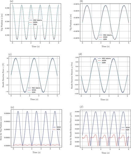
The proposed Winkler foundation model was solved using both the DDM and the RFEM approaches, as well as MSC Adams. The stiffness constant was chosen as , based on the values reported by Glozman and Shoham [Citation81], while the damping ratio was chosen as
, based on the estimated stiffness-to-damping ratio for soft tissues reported by Khadem et al. [Citation14]. It should be noted that these values are used for providing a qualitative approximation of the types of forces that are present during needle insertion procedures and do not aim to provide an accurate tissue model. The distributed loading was approximated with the help of evenly distributed points that spanned half of the needle’s length. For this simulation, the needle’s rigid base was constrained to follow an arbitrary trajectory
where , with
and
. The simulation times are indicative of the time required for a single sample acquisition in LATP procedures. The simulation results are illustrated in .
Figure 19. (a) Response of tip’s position in direction. (b) Response of tip’s position in z direction. (c) Reaction force at needle’s handle in z direction. (d) Reaction moment at needle’s handle in y direction. (e) Error
for the tip position. (f) Error
for the handle force.
4. Discussion
The simulation results presented in Section 3 allow for a direct accuracy and efficiency comparison between the different modelling approaches. As shown in , linear modelling techniques pose significant limitations for capturing the deflection profile of the flexible needle in the case of large deformations. More specifically, the linear Ansys solver remains valid only for small deformations (), while in the case of large needle deflections (), the linear approach leads to unrealistic and non-volume preserving deflection profiles. On the other hand, as illustrated in the same figures, due to their inherent geometric nonlinearity, both the DDM and the RFEM methods lead to highly accurate deflection profiles even for large needle deformations. This is also illustrated in , in which the DMM and the RFEM methods lead to a near-zero value of the performance measure of Equationequation (41)(41)
(41) , while the linear approach leads to significant errors especially for large needle deflections. Due to their poor accuracy, linear solutions were not included in the subsequent investigations.
The second simulation scenario was designed to provide insight into the dynamic behaviour of the proposed modelling approaches. As illustrated in , both the DDM and RFEM approaches capture the vibrational behaviour of the needle with high accuracy and quickly converge to the desired solution, leading to a close to zero deviation from the MSC Adams simulation results. It should be noted that both the equations of motion and the associated algorithms were structured in an identical way for the two methods, which allowed the implementation of direct efficiency comparisons between them. As shown in , while both methods can be used for acquiring real-time solutions, the DDM method leads to significantly higher execution times compared to the RFEM (for the same accuracy level). More specifically, comparison of the mean error in reveals that for the examined simulation the RFEM approach allows real-time execution using a discretization of up to six elements. On the contrary, a real-time simulation using the DDM approach can only be achieved with no more than three elements, resulting in a comparatively lower accuracy of the method. The same observations can be made for the mean error
illustrated in . The performance difference between the two methods can be partly attributed to the fact that DDM requires twice the number of DOFs per element than the RFEM. Additionally, it was observed that, during the implicit integration of the equations of motion, the DDM method generally required more iterations of the inner Newton–Raphson for the solution’s convergence, especially in the cases where a rigid body motion was imposed on the system. Further analysis of the system revealed that the source of the numerical problems, which led to more iterations, was inherent to the method as a large condition number was observed on the generalized strain Jacobian defined in Equationequation (11)
(11)
(11) . On the other hand, the RFEM method showed superior numerical behaviour allowing fast integration and stable solutions even with the use of semi-implicit integration schemes that can further improve the overall system’s performance. Furthermore, the sparse structure of the system’s matrices and the property of the RFEM algorithm for destructuring and concurrent execution allowed further optimizations on the system’s numerical efficiency.
The third simulation scenario was designed to analyse the effect of complex loading conditions and driving constraints that resemble those encountered during actual needle insertion procedures. As illustrated in , both methods captured the needle dynamics with high accuracy, leading to negligible errors for both the tip position and the reaction force at the surgeon’s hand. It should be noted that the performance plots for this simulation scenario followed a similar structure to the ones presented in . More specifically, both methods allowed real-time execution, with the RFEM outperforming the DDM method in terms of computational efficiency. In both dynamic simulations, the execution-time-to-real-time ratio reported by MSC Adams was close to one. However, as the software does not give the user the ability to extract the exact details of the numerical solution, these results have not been reported in .
A systematic investigation of the different FMD modelling approaches reveals that the RFEM method constitutes one of the most optimal candidates for providing robust and accurate solutions for the examined problem. The properties of the RFEM algorithm, combined with the proposed solution strategy (optimized to the particular properties of the problem) allow high computational efficiency and real-time execution capabilities without the need for modelling assumptions that compromise the overall system’s accuracy. Furthermore, even though the parametric nature of our models allows its application to a variety of needle insertion procedures, our focus remains on long, slender and moderately flexible needles, such as the ones used in LATP and prostate brachytherapy procedures.
It should be noted that the computational times reported in the previous examples do not take into account the deformation of the surrounding tissue, but they solely refer to the computational effort for capturing the needle’s deflection under a generalized force field that quantitatively emulates the one encountered during needle insertion procedures. Ensuring numerical stability and accuracy when modelling soft tissues undergoing large localized strain induced by the needle is the remaining part of the challenge, as tissue modelling is a highly challenging modelling and computational endeavour. The identification of the tissue properties, the proper modelling of fracture and contact dynamics and the treatment of spatial discontinuities during needle insertion constitute open modelling challenges.
However, this work studies the needle’s dynamic model and its vibrational behaviour independent of the tissue and their interaction. It does not attempt to solve the whole problem of needle insertion, but it attempts to provide high fidelity models for the needle’s dynamics. Such needle models, are invaluable for identifying the properties of needle insertion as the needle can be seen as a filter through which the generalized needle–tissue interaction forces can be measured.
5. Conclusions
In this paper, we presented two novel three-dimensional dynamic rigid/flexible models of brachytherapy and LATP needles under a general 3D force field. The proposed models were chosen based on a thorough investigation of different FMD methods and their ability to tackle the numerical particularities of thin flexible medical needles. By employing the theory of FMD and incorporating methods that account for geometric nonlinearities, the proposed approaches minimized the need for introducing modelling assumptions that could compromise their performance. They provided a complete characterization of the system’s rigid motion and vibrational behaviour for both small and large deformations and allowed the correlation of the system’s state with input parameters, such as insertion velocity and needle orientation.
Furthermore, this work presented a novel simulation algorithm, based on the generalized recursive Newton–Euler formulation that characterized and quantified the correlation between the system’s inertial and external forces with the generalized reaction forces acting on its base. The proposed algorithm, tailored to the requirements of the specific application, was combined with parallel architecture implementation strategies to allow for computationally efficient solutions and real-time execution.
The models were assessed in terms of accuracy and computational efficiency and their performance was validated with the help of commercial simulation software. It was shown that linear approaches lead to significant limitations and are not suitable for providing accurate and realistic solutions. On the other hand, both of the employed nonlinear approaches presented high levels of accuracy for both static and dynamic system responses. The RFEM method is shown to be more robust and numerically efficient than the DMM method, and is recommended as the proposed technique for further investigations on medical needle dynamics.
Future work will further analyse the RFEM model in order to validate its performance in experimental studies. The model will also be used in conjunction with computationally efficient and accurate tissue models and will act as the basis for modelling the dynamics of virtual surgical instruments of a fully featured medical simulation solution. Future extensions of our work will also allow the implementation of the proposed model with the help of the graphics processing unit, aiming at further improvement of the model’s computational efficiency.
Disclosure statement
The authors declare that they have no known competing financial interests or personal relationships that could have appeared to influence the work reported in this paper.
Additional information
Funding
References
- A.M. Okamura, C. Simone, and M.D. O’Leary, Force modeling for needle insertion into soft tissue, IEEE Trans. Biomed. Eng. 51 10 (Oct 2004), pp. 1707–1716. doi:10.1109/TBME.2004.831542
- G. Ravali and M. Muniyandi, Haptic feedback in needle insertion modeling and simulation: Review. IEEE Reviews in Biomedical Engineering. 10 (2017), pp. 63–77.
- N. Abolhassani, R. Patel, and M. Moallem, Needle insertion into soft tissue: A survey, Med Eng Phys 29 (4) (2007), pp. 413–431. doi:10.1016/j.medengphy.2006.07.003.
- H.S. Bassan, R.V. Patel, and M. Moallem, A novel manipulator for percutaneous needle insertion: Design and experimentation, IEEE/ASME Trans J. Mechatron. 14 6 (Dec 2009), pp. 746–761. doi:10.1109/TMECH.2009.2011357
- J. Yanof, J. Haaga, P. Klahr et al., CT-integrated robot for interventional procedures: Preliminary experiment and computer-human interfaces, Comput. Aided Surg. 6 (6) (2001), pp. 352–359. doi:10.3109/10929080109146304.
- J. Hing, A. Brooks, and J. Desai, Reality-based needle insertion simulation for haptic feedback in prostate brachytherapy. In: Proceedings 2006 IEEE International Conference on Robotics and Automation, 2006. ICRA 2006, Orlando, FL, USA. (2006), pp. 619–624.
- O. Goksel, K. Sapchuk, and S.E. Salcudean, Haptic simulator for prostate brachytherapy with simulated needle and probe interaction, IEEE Trans Haptics. 4(3), (Jul 2011), pp. 188–198. doi:10.1109/TOH.2011.34
- O. Goksel, E. Dehghan, and S.E. Salcudean, Modeling and simulation of flexible needles, Med Eng Phys 31 (9) (2009), pp. 1069–1078. doi:10.1016/j.medengphy.2009.07.007.
- S.P. DiMaio and S.E. Salcudean, Needle insertion modeling and simulation, IEEE Trans. Robot. Autom. 19 5 (Oct 2003), pp. 864–875. doi:10.1109/TRA.2003.817044
- M. Freutel, H. Schmidt, L. Dürselen et al., Finite element modeling of soft tissues: Material models, tissue interaction and challenges, Clin Biomech 29 (4) (2014), pp. 363–372. doi:10.1016/j.clinbiomech.2014.01.006.
- H. Delingette, Toward realistic soft-tissue modeling in medical simulation, Proceedings of the IEEE. 86 (3), (1998), pp. 512–523.
- S. Jiang, P. Li, Y. Yu et al., Experimental study of needle–tissue interaction forces: Effect of needle geometries, insertion methods and tissue characteristics, J. Biomech. 47 (13) (2014), pp. 3344–3353. doi:10.1016/j.jbiomech.2014.08.007.
- L. Barbé, B. Bayle, M. De Mathelin et al., Needle insertions modeling: Identifiability and limitations, Biomed. Signal Process. Control 2 (3) (2007), pp. 191–198. doi:10.1016/j.bspc.2007.06.003.
- M. Khadem, C. Rossa, N. Usmani et al., A two-body rigid/flexible model of needle steering dynamics in soft tissue, IEEE/ASME Trans J. Mechatron. 21 (5) (Oct 2016), pp. 2352–2364. doi:10.1109/TMECH.2016.2549505
- T. Lehmann, C. Rossa, N. Usmani et al., A real-time estimator for needle deflection during insertion into soft tissue based on adaptive modeling of needle–tissue interactions, IEEE/ASME Trans J. Mechatron. 21 (6) (Dec 2016), pp. 2601–2612. doi:10.1109/TMECH.2016.2598701
- R.J. Webster I, J.S. Kim, N.J. Cowan et al., Nonholonomic modeling of needle steering, Int J Rob Res 25 (5–6) (2006), pp. 509–525. doi:10.1177/0278364906065388.
- G.J. Vrooijink, M. Abayazid, S. Patil et al. Needle path planning and steering in a three-dimensional non-static environment using two-dimensional ultrasound images, Int J Rob Res.3310 (20149), pp. 1361–1374 10.1177/0278364914526627
- Y. Zhang, Z. Ju, H. Zhang et al., 3-d path planning using improved rrt* algorithm for robot-assisted flexible needle insertion in multilayer tissues, IEEE Can. J. Electr. Comput. Eng. 12 (2021), pp. 1–13.
- A. Asadian, M.R. Kermani, and R.V. Patel, An analytical model for deflection of flexible needles during needle insertion. In: 2011 IEEE/RSJ International Conference on Intelligent Robots and Systems, San Francisco, CA, USA. (Sep 2011), pp. 2551–2556.
- N. Abolhassani, R.V. Patel, and F. Ayazi, Minimization of needle deflection in robot-assisted percutaneous therapy, Int. J. Med. Robot. Comput. Assist Surg 3 (2) (2007), pp. 140–148. doi:10.1002/rcs.136.
- K.E. Bisshopp and D.C. Drucker, Quarterly of Applied Mathematics, Large deflection of cantilever beams. 3 (1945), pp. 272–275.
- S.P. DiMaio and S.E. Salcudean, Interactive simulation of needle insertion models, IEEE Trans. Biomed. Eng. 52 7 (Jul 2005), pp. 1167–1179. doi:10.1109/TBME.2005.847548
- Y. Adagolodjo, L. Goffin, M. De Mathelin et al. Robotic insertion of flexible needle in deformable structures using inverse finite-element simulation, IEEE Trans Rob. 353 (20196), pp. 697–708 10.1109/TRO.2019.2897858
- A. Haddadi and K. Hashtrudi-Zaad, Development of a dynamic model for bevel-tip flexible needle insertion into soft tissues. Conference proceedings: Annual International Conference of the IEEE Engineering in Medicine and Biology Society IEEE Engineering in Medicine and Biology Society Conference, Boston, Massachusetts, USA. 2011 (2011), pp. 7478–7482.
- T. Podder, D. Clark, D. Fuller et al., Effects of velocity modulation during surgical needle insertion. In: 2005 IEEE Engineering in Medicine and Biology 27th Annual Conference, Shanghai, China. (2005), pp. 5766–5770.
- T. Podder, D. Clark, J. Sherman et al., In vivo motion and force measurement of surgical needle intervention during prostate brachytherapy, Med. Phys. 33 (8) (2006), pp. 2915–2922. doi:10.1118/1.2218061.
- L. Tan, X. Qin, Q. Zhang et al., Effect of vibration frequency on biopsy needle insertion force, Med Eng Phys 43 (2017), pp. 71–76. doi:10.1016/j.medengphy.2017.02.011.
- C. McGill, J. Schwartz, J. Moore et al., Effects of insertion speed and trocar stiffness on the accuracy of needle position for brachytherapy, Med. Phys. 39 (4) (2012), pp. 1811–1817. doi:10.1118/1.3689812.
- M. Abayazid, M. Kemp, and S. Misra, 3D flexible needle steering in soft-tissue phantoms using Fiber Bragg Grating sensors. In: 2013 IEEE International Conference on Robotics and Automation, Karlsruhe, Germany. (May 2013), pp. 5843–5849.
- N. Abolhassani, R. Patel, and F. Ayazi, Effects of different insertion methods on reducing needle deflection. In: 2007 29th Annual International Conference of the IEEE Engineering in Medicine and Biology Society, Lyon, France. (Aug 2007), pp. 491–494.
- R. Tsumura, Y. Takishita, and H. Iwata, Needle insertion control method for minimizing both deflection and tissue damage. Journal of Medical Robotics Research. 4 (1), (2019), pp. 1842005.
- N.A. Wood, K. Shahrour, M.C. Ost et al., Needle steering system using duty-cycled rotation for percutaneous kidney access. In: 2010 Annual International Conference of the IEEE Engineering in Medicine and Biology, Buenos Aires, Argentina. 8 (2010), pp. 5432–5435.
- S. Badaan, D. Petrisor, C. Kim, Does needle rotation improve lesion targeting?, The International Journal of Medical Robotics + Computer Assisted Surgery: MRCAS. 7 (2), (2011), pp.138–147. doi:10.1002/rcs.381.
- A. Martsopoulos, P. Rajendra, B. Stefanos et al., Spatial rigid/flexible dynamic model of biopsy and brachytherapy needles under a general force field. In: 2020 IEEE International Conference on Intelligent Robots and Systems (IROS), Las Vegas, NV, USA. (Oct 2020).
- E. Wittbrodt, I. Adamiec-Wójcik, and S. Wojciech, Dynamics of Flexible Multibody Systems: Rigid Finite Element Method. Springer, Foundations of Engineering Mechanics, Berlin Heidelberg, (2007).
- A.A. Shabana, Flexible multibody dynamics: Review of past and recent developments, Multibody Syst Dyn. 1 2 (Jun 1997), pp. 189–222. doi:10.1023/A:1009773505418
- J.M. Mayo, D. García-Vallejo, and J. Domínguez, Study of the geometric stiffening effect: Comparison of different formulations, Multibody Syst Dyn. 11 4 (May 2004), pp. 321–341. doi:10.1023/B:MUBO.0000040799.63053.d9
- A. Shabana, Dynamics of Multibody Systems, Cambridge, England: Cambridge University Press, 2003.
- E.M. Bakr and A.A. Shabana, Geometrically nonlinear analysis of multibody systems, Comput Struct. 23 6 (Jan 1986), pp. 739–751. doi:10.1016/0045-7949(86)90242-7
- J. Mayo, J. Domínguez, and A. Shabana, Geometrically nonlinear formulations of beams in flexible multibody dynamics, J Vib Acoust. 117 4 (Oct 1995), pp. 501–509. doi:10.1115/1.2874490
- I. Sharf, Geometrically Non-Linear Beam Element for Dynamics Simulation of Multibody Systems, Int J Numer Methods Eng 39 (5) (1996), pp. 763–786. doi:10.1002/(SICI)1097-0207(19960315)39:5<763::AID-NME879>3.0.CO;2-X.
- U. Lugrís, M. Naya, J. Pérez et al., Implementation and efficiency of two geometric stiffening approaches, Multibody Syst Dyn. 20 (2) (Sep 2008), pp. 147–161. doi:10.1007/s11044-008-9114-6
- A. Nada, B. Hussein, S. Megahed, Use of the floating frame of reference formulation in large deformation analysis: Experimental and numerical validation, Proceedings of the Institution of Mechanical Engineers, Part K: Journal of Multi-body Dynamics. 224 (1), (Mar 2010). pp. 45–58.
- J.N. Reddy, An Introduction to Nonlinear Finite Element Analysis Second Edition: With Applications to Heat Transfer, Fluid Mechanics, and Solid Mechanics, Oxford, England: OUP Oxford, 2014.
- A.A. Shabana, Computational Continuum Mechanics, Cambridge, England: Cambridge University Press, 2008.
- A. Shabana, An Absolute Nodal Coordinate Formulation for the Large Rotation and Deformation Analysis of Flexible Bodies, Chicago, Illinois: Department of Mechanical and Industrial Engineering, University of Illinois at Chicago, 1996.
- A.A. Shabana and R.Y. Yakoub, Three dimensional absolute nodal coordinate formulation for beam elements: Theory, Mech. Eng. J. 123 4 (May 2000), pp. 606–613. doi:10.1115/1.1410100
- J. Sopanen and A. Mikkola, Studies on the stiffness properties of the absolute nodal coordinate formulation for three-dimensional beams, European Journal of Ophthalmology 13 (Suppl. 3) (2003), pp. 0. doi:10.5301/EJO.2008.4238.
- B.A. Hussein, H. Sugiyama, and A.A. Shabana, Coupled deformation modes in the large deformation finite-element analysis: Problem definition, J. Comput. Nonlinear Dyn. 2 2 (Nov 2006), pp. 146–154. 1. doi:10.1115/1.2447353
- A. Schwab and J. Meijaard, Comparison of three-dimensional flexible beam elements for dynamic analysis: Classical finite element formulation and absolute nodal coordinate formulation, J. Comput. Nonlinear Dyn. 51 (2010 Jan; 5), 10.1115/1.4000320.
- J. Sopanen and A. Mikkola, Description of elastic forces in absolute nodal coordinate formulation, Nonlinear Dyn. 34 1/2 (Oct 2003), pp. 53–74. doi:10.1023/B:NODY.0000014552.68786.bc
- J. Gerstmayr and A.A. Shabana, Analysis of thin beams and cables using the absolute nodal co-ordinate formulation, Nonlinear Dyn. 45 1 (Jul 2006), pp. 109–130. doi:10.1007/s11071-006-1856-1
- P.G. Gruber, K. Nachbagauer, Y. Vetyukov et al., A novel director-based Bernoulli–Euler beam finite element in absolute nodal coordinate formulation free of geometric singularities, Int. J. Mech. Sci. 42 (2013 Aug; 4), pp. 279–289 10.5194/ms-4-279-2013
- S. von Dombrowski, Analysis of large flexible body deformation in multibody systems using absolute coordinates, Multibody Syst Dyn. 8 4 (Nov 2002), pp. 409–432. doi:10.1023/A:1021158911536
- J.B. Jonker and J.P. Meijaard, A geometrically non-linear formulation of a three-dimensional beam element for solving large deflection multibody system problems, Int J Non Linear Mech. 53 (2013), pp. 63–74. doi:10.1016/j.ijnonlinmec.2013.01.012
- H. Kaminski and P. Fritzkowski, Application of the rigid finite element method to modelling ropes, Lat. Am. J. Solids Struct. 10 (1) (2013), pp. 91–99. doi:10.1590/S1679-78252013000100009.
- I. Adamiec-Wójcik, J. Awrejcewicz, L. Brzozowska, Modelling of ropes with consideration of large deformations and friction by means of the rigid finite element method. Springer Proceedings in Mathematics & Statistics. 93 (2014), pp. 115–137.
- M.A. Gorin, A.R. Meyer, M. Zimmerman et al., Transperineal prostate biopsy with cognitive magnetic resonance imaging/biplanar ultrasound fusion: Description of technique and early results, World J Urol. 388 (20208), pp. 1943–1949. doi:10.1007/s00345-019-02992-4.
- C. Rossa and M. Tavakoli, Issues in closed-loop needle steering, Control Eng. Pract. 62 (2017), pp. 55–69. doi:10.1016/j.conengprac.2017.03.004.
- N. Chentanez, R. Alterovitz, D. Ritchie et al., ACM Transactions on Computer Systems, Interactive simulation of surgical needle insertion and steering. 28 (3), (2009). pp. 1–10.
- D. Gao, Y. Lei, B. Lian et al., Modeling and simulation of flexible needle insertion into soft tissue using modified local constraints, J Manuf Sci Eng. 138 (12), (2016), pp. 1167–1175.
- J. Xu, L. Wang, K.C.L. Wong et al. A meshless framework for bevel-tip flexible needle insertion through soft tissue. In: 2010 3rd IEEE RAS EMBS International Conference on Biomedical Robotics and Biomechatronics, Tokyo, Japan. (Sep 2010). p. 753–758.
- L. Wang and S. Hirai, A local constraint method for needle insertion modeling and simulation. In: 2011 IEEE International Workshop on Haptic Audio Visual Environments and Games, Qinhuangdao, China. (Oct 2011). p. 39–44. null.
- A. Asadian, M.R. Kermani, and R.V. Patel, A compact dynamic force model for needle-tissue interaction. In: 2010 Annual International Conference of the IEEE Engineering in Medicine and Biology, Buenos Aires, Argentina. (Aug 2010). p. 2292–2295.
- K. Yan, T. Podder, D. Xiao et al., An improved needle steering model with online parameter estimator, Int. J. Comput. Assist. Radiol. Surg. 1 (4) (2006), pp. 205–212. doi:10.1007/s11548-006-0058-0.
- A. Asadian, R.V. Patel, and M.R. Kermani, A distributed model for needle-tissue friction in percutaneous interventions. In: 2011 IEEE International Conference on Robotics and Automation, Shanghai, China. (May 2011). p. 1896–1901.
- H. Yang, P.X. Liu, and J. Zhang, Modelling of needle insertion forces for surgical simulation. In: IEEE International Conference Mechatronics and Automation, 2005, Niagara Falls, ON, Canada. 2 (Jul 2005). p. 592–595.
- M. Khadem, C. Rossa, R.S. Sloboda et al., Mechanics of tissue cutting during needle insertion in biological tissue, IEEE Robot. Autom. Lett. 1 (2) (Jul 2016), pp. 800–807. doi:10.1109/LRA.2016.2528301
- P. Li, S. Jiang, Y. Yu et al., Biomaterial characteristics and application of silicone rubber and PVA hydrogels mimicked in organ groups for prostate brachytherapy, J Mech Behav Biomed Mater. 49 (2015), pp. 220–234.
- B. Zhao, L. Lei, L. Xu et al. Needle deflection modeling and preoperative trajectory planning during insertion into multilayered tissues. IEEE/ASME Transactions on Mechatronics, 262 (2021-04), pp. 943–954.
- W. Durham, Aircraft Flight Dynamics and Control Aerospace Series, Hoboken, New Jersey: John Wiley & Sons, 2013.
- J.P. Meijaard, Validation of flexible beam elements in dynamics programs, Nonlinear Dyn. 9 1 (Feb 1996), pp. 21–36. doi:10.1007/BF01833291
- W.S. Yoo, O. Dmitrochenko, and D. Pogorelov, Review of finite elements using absolute nodal coordinates for large-deformation problems and matching physical experiments. ASME 2005 International Design Engineering Technical Conferences and Computers and Information in Engineering Conference, Long Beach, California, USA, 6 (2005), pp. 1285–1294.
- A. Shabana, Computational Dynamics, Hoboken, New Jersey, U.S.: Wiley, 2001.
- A.A. Shabana, Dynamics of flexible bodies using generalized Newton-Euler equations, J Dyn Syst Meas Control. 112 (09 1990), pp.496–503. 10.1115/1.2896170
- I. Elgezua, Y. Kobayashi, and M.G. Fujie, Estimation of needle tissue interaction based on non-linear elastic modulus and friction force patterns. In: 2014 IEEE/RSJ International Conference on Intelligent Robots and Systems, Chicago, IL, USA. (Sep 2014). p. 4315–4320.
- E. Hairer and G. Wanner, Solving Ordinary Differential Equations Ii: Stiff and differential-algebraic Problems, Springer, Berlin Heidelberg, 2010. ( Springer Series in Computational Mathematics).
- C. Sanderson and R. Curtin, Armadillo: A template-based c++ library for linear algebra, J. Open Source Softw. 1 (2) (2016), pp. 26. doi:10.21105/joss.00026.
- L. Dagum and R. Menon, OpenMP: An industry-standard API for shared-memory programming, IEEE Comput. Sci. Eng. 5 1 (Jan 1998), pp. 46–55. doi:10.1109/99.660313
- C.S. Yim and A.K. Chopra, Earthquake response of structures with partial uplift on Winkler foundation, Earthq. Eng. Struct. Dyn. 12 (2) (1984), pp. 263–281. doi:10.1002/eqe.4290120209.
- D. Glozman and M. Shoham, Image-guided robotic flexible needle steering, IEEE Trans Rob. 23 3 (Jun 2007), pp. 459–467. doi:10.1109/TRO.2007.898972
- K. Yan, T. Podder, Y. Yu et al. Flexible needle-tissue interaction modeling with depth-varying mean parameter: Preliminary study. ichange1 IEEE Trans. Biomed. Eng. 56 (2009), pp. 255–262.
- H. Lee and J. Kim, Estimation of flexible needle deflection in layered soft tissues with different elastic moduli, Med. Biol. Eng. Comput. 52 (2014), pp. 729–740.