Mathematical modelling of an electrostatic oiling machine for steel strips

ABSTRACT

This paper deals with the mathematical modelling of the electrostatic spraying process in an industrial electrostatic oiling machine (EOM) for steel strips. Measurements from an industrial EOM show that the thickness and inhomogeneity of the oil film on the strips frequently exceed specified tolerance limits whereby the reasons were previously unknown. A numerical model of the spraying process is developed in ANSYS Fluent, which serves as the basis for a root-cause analysis of the erroneous oil film thickness. In contrast to other works in this area, a droplet break-up model, which describes the break-up of the oil droplets due to the charge they carry, is included to get more accurate results. The model is validated based on measurement data from an industrial oiling machine. It is demonstrated that the model yields a better understanding of the spraying process and it is successfully used to improve the oiling process.

KEYWORDS:

• Electrostatic coating
• oiling machine
• oil droplets
• numerical model
• steel strip
• Hot-dip galvanizing

1. Introduction

Spraying is used in many industrial applications such as powder coating, painting, or oiling as presented here. Electrostatic spraying systems are more efficient in terms of deposition at the target surface than systems that use brushes, rollers, or airsprays. This paper deals with an electrostatic oiling machine which is part of a hot-dip galvanizing line of voestalpine in Linz, Austria, where steel strips are protected against corrosion. After the zinc coating is solidified, an oil film is applied to passivate the surface.

Some of the main components of the hot-dip galvanizing line are sketched in Figure 1.

Figure 1. Main components of the considered hot-dip galvanizing line.

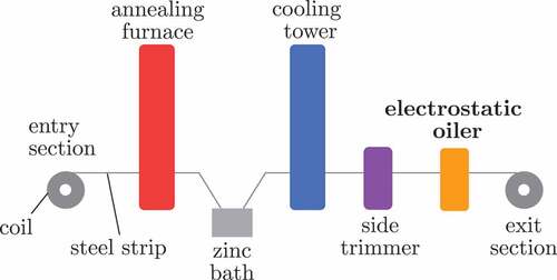
In the entry section, the steel coils are decoiled and joined together to an endless strip. In the furnace, the strip is annealed to prepare its surface for the subsequent coating process [1]. The steel strip surface is coated by conveying it through the molten zinc in the zinc bath. The liquid zinc layer solidifies in the subsequent cooling tower.

The side trimmer cuts the strip to the desired width and the resulting scrap is removed. In the electrostatic oiling machine (EOM), oil is atomized and sprayed onto both sides of the steel strip due to a high electrostatic field strength. The oil film on the steel strip passivates the surface and acts also as a lubricant in subsequent forming processes. In the exit section, the endless steel strip is cut into pieces that are then finally coiled. The thickness of the oil film on the strip surface must lie within specified limits and should be as homogeneous as possible. Measurements of the thickness distribution of the oil film show that this is not always fulfilled. The reasons were previously unknown. In the course of this work, a mathematical model is developed and used to identify possible reasons for a non-uniform oil film thickness on the strip and to improve the oiling process.

Electrostatic oiling is a complex, nonlinear multiphysics problem with a two-phase fluid flow and distributed parameters (infinite-dimensional system). In this paper, a numerical, two-dimensional, steady-state model of the electrostatic spraying process for a specific type of EOM is developed. It is used to improve the understanding of the process, to identify the dependence of the output variables on the input variables and parameters of the system, and to identify possibilities for optimization.

Models of the type of EOM considered in this paper are rarely published. However, there are some articles that present mathematical models of electrostatic spraying processes. A finite-element method (FEM) model of an electrostatic rotary bell atomizer is presented in [2]. A numerical method developed for the calculation of the electric field and the particle trajectories for electrostatic powder coating can be found in [3]. ANSYS Fluent with user-defined functions is used to evaluate the electrostatic field under consideration of the space charge. In [4], a three-dimensional numerical ANSYS Fluent model of an electrostatic coating process that incorporates a moving mesh to simulate movements of the target object is presented. A numerical study on spray painting processes using three different atomizers, i.e. a high-speed rotary bell atomizer, an airless gun, and a pneumatic air spray gun, is presented in [5]. The implementation of an electric field in ANSYS Fluent by means of user-defined functions is described in more detail in [6]. In [3–5] a specific size distribution is considered for the injected particles to get more accurate results.

None of the mentioned models considers a break-up of the particles. However, based on measurements, it was found that in the present spraying process, break-ups of the oil droplets on their way from the oiling blades to the steel strip occur. This is due to the repelling forces between the charges carried by the droplets and due to the drag force. These break-ups influence the trajectories of the oil droplets and the opening angle of the oil spray. The scientific novelty of this work is that, in contrast to other works in this area, a droplet break-up submodel is included to obtain more accurate calculation results. This is necessary to get valid simulation results used for the improvement of the spraying process regarding the distribution of the oil film thickness.

This paper is organized as follows. Section 2 describes the main components of the considered EOM and their function. The numerical model implemented in ANSYS Fluent and the underlying equations are presented in Section 3. Section 4 describes the measurements that were carried out, the parameter identification, and the model validation. Some simulation results are summarized in Section 5. Section 6 shows a case study where the model is used to optimize the angular orientation of the upper oiling blade. Section 7 provides some conclusions.

2. Description of the EOM

This chapter describes the main components of the considered EOM. Figure 2 shows the two-blade EOM for the coating of continuously moving strips. This type of EOM consists of two opposing oiling blades supplied with high voltage and an electrically insulating enclosure. The steel strip is electrically grounded. The high voltage in combination with the blade geometry leads to a high electric field strength at the blade edge. The steel strip is continuously conveyed through the enclosure and in this way oiled on both sides. The protection plates protect the blades in case of loss of strip tension or when the upstream trimming of the strip is faulty and some of the strip scrap runs into the EOM. The oil has a high viscosity at ambient temperature and therefore adheres well to the surface of the steel strip.

Figure 2. Electrostatic oiling machine. (a) Cross section. (b) Front view of the electrostatic oiling blades.

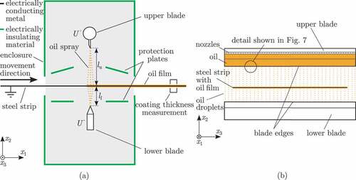
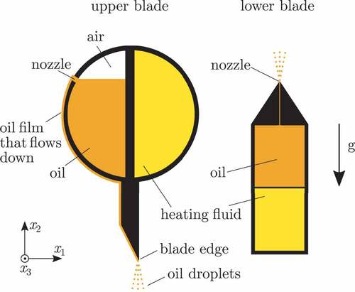
In an external tank, the oil is stored and heated up to a temperature of about 30°C to lower its viscosity. From there, pumps deliver the oil to the blades, which have two cavities each. The oil is pumped into one of them. A heating fluid with a temperature of 70°C is circulating through the other cavity and thereby heats up the oil. This is illustrated in Figure 3. An oil temperature of 70°C is necessary to get a good atomization behaviour. The heated oil flows through the nozzles and reaches the blade edge. At the upper blade, the oil film flows down on the surface of the blade by means of gravity. At the blade edges, the oil is charged and atomized due to the high electric field strength. After the atomization, the oil droplets leave the blade edge towards the strip surface which is kept at ground potential. The oil droplets are accelerated by the electrostatic force. Since the width of the strips is lower than the length of the blades (cf. Figure 2(b)), some of the oil droplets do not hit the strip. To prevent both a loss of oil through the openings of the enclosure or overoiling of the strip edges, the upper and the lower blade voltages are of opposite polarity, which implies that the corresponding droplets are oppositely charged. These droplets meet and electrically neutralize each other left and right of the strip before they fall down into a bottom sump. The excess oil is collected there and pumped back into the tank.

Figure 3. Cross section of the oiling blades.

Downstream of the EOM, the thickness distribution of the oil film is measured without contact using laserinduced fluorescence spectroscopy. This measurement system monitors if the oil film thickness is outside its tolerance limits. In particular for these situations, the mathematical model developed in Section 3 gives valuable insights for a root-cause analysis of the erroneous oil film thickness. Moreover, the model serves as the basis to identify possibilities for optimization and improvement of the oiling process, e.g. regarding the uniformity of the oil film thickness.

3. Mathematical model

This section presents the theoretical background and the equations used in the numerical, two-dimensional, two-phase, steady-state model of the considered EOM. Only the steady state is considered because the operating conditions are usually kept constant.

The model calculates the electric field, the airflow, and the droplet trajectories inside the enclosure of the EOM. The model does not take the oil film on the oiler blades into account, but starts right after the atomization at the blade tips. The input variables of the model are the voltages $U$ applied between the blades and the strip, the mass flow rate $Q$ of the oil that is pumped to the blades, and the velocity $v_{strip}$ of the steel strip.

The electric current $I$ that flows from the blade to the strip and the mean radius $r_0$ of the droplets right after atomization depend on the voltage $U$, the oil mass flow rate $Q$, the blade geometry, the distance between the blade and the strip, and the oil properties. The atomization process of the oil at the blade edges could be modelled in detail to get functions of the form $I(U,Q,\dots )$ and $r_0(U,Q,\dots )$. Such a model for $I$ and $r_0$ would significantly increase the complexity and the computational effort of the overall model. This is why in this work, the current $I$ and the droplet radius $r_0$ are simply measured and used as additional input variables of the model. Consequently, with this model the spraying process can be simulated for all measured operating points. The developed model with measured inputs for $I$ and $r_0$ is sufficient to satisfy the stated objectives.

A block diagram of the included physical quantities and their couplings is shown in Figure 4.

Figure 4. Block diagram of the model.

The submodel of the airflow and the submodel of the droplets are coupled via the drag force acting on the droplets. The submodel of the electric field and the submodel of the droplets are coupled via the electrostatic force acting on the charge carried by the droplets. The current caused by the movement of the charged oil droplets is very low and thus the generated magnetic field and its effect on the trajectories is negligible.

Due to the independence of the calculation results along the spatial direction $x_3$ (see Figure 2) and in favour of the computational effort, only the $x_1$-$x_2$-plane according to Figure 2(a) is considered in the model. However, for the sake of completeness, the three-dimensional equations are given in the following. For scalar components, the indices $i,j=1,2,3$ are used. Vector quantities are written in bold. Taking into account the associated boundary conditions, the following equations apply to both the upper and the lower part of the EOM. In the following equations, the coordinates $x_i$ are restricted to the domain within the EOM (see grey shaded box in Figure 2(a)).

3.1. Electric field

The electric field which is generated by the charged oil droplets and the voltage applied between the oiling blades and the strip is governed by Poisson’s equation [7].

(1) $\frac{{\mathrm{\partial }}^2\phi }{\mathrm{\partial }{x}_i^2}=\frac{{\rho }_e}{\in }$(1)

where $\phi$ is the electric potential, ${\rho }_e$ is the charge density, and $\in$ is the electrical permittivity of air.

The electric field $\mathbf{E}$ follows from

(2) $E_i=-\frac{\mathrm{\partial }\phi }{\mathrm{\partial }{x}_i}$(2)

The boundary conditions are $\phi =0$ at the strip and $\phi =U^{+}$ and $\phi =U^{-}$ at the upper and the lower blade, respectively. At the (electrically insulating) enclosure of the EOM, the normal component ${\mathbf{E}}_{\mathrm{\perp }}$ of the electric field is set to zero. The applied voltages $U^{+}$ and $U^{-}$ are constant over time.

3.2. Airflow

The airflow inside the EOM induced by the movement of the oil droplets and of the steel strip constitutes a classical fluid dynamics problem and is calculated based on the momentum and mass conservation equations. The mass conservation also known as continuity equation reads as [8]

(3) $\frac{\mathrm{\partial }\rho }{\mathrm{\partial }t}+\frac{\mathrm{\partial }}{\mathrm{\partial }{x}_i}(\rho v_i)=0$(3)

where $\rho$ is the mass density of air and $\mathbf{v}$ is its velocity. Since in the EOM the airflow velocity is much smaller than the speed of sound and consequently the Mach-number is much smaller than one, the fluid can be treated as incompressible and (3) reduces to [8]

(4) $\frac{\mathrm{\partial }{v}_i}{\mathrm{\partial }{x}_i}=0$(4)

The momentum conservation equations, also known as Navier-Stokes equations, for incompressible flows read as [8]

(5) $\frac{\mathrm{\partial }{v}_i}{\mathrm{\partial }t}+v_j\frac{\mathrm{\partial }{v}_i}{\mathrm{\partial }{x}_j}=-\frac{1}{\rho }\frac{\mathrm{\partial }p}{\mathrm{\partial }{x}_i}+\nu \frac{{\mathrm{\partial }}^2{v}_i}{\mathrm{\partial }{x}_j^2}-g{\delta }_{i,2}+f_i$(5)

where $p$ is the pressure, $\nu$ is the kinematic viscosity of air, $g$ is the gravitational acceleration and $\mathbf{f}$ contains all the external body forces in general. Here, $\mathbf{f}$ is the drag force (per unit mass) caused by the movement of the droplets and will be formulated in (20). The Kronecker ${\delta }_{i,2}$ equals one for $i=2$ and is zero otherwise. The Navier-Stokes equations (5)(5) $\frac{\mathrm{\partial }{v}_i}{\mathrm{\partial }t}+v_j\frac{\mathrm{\partial }{v}_i}{\mathrm{\partial }{x}_j}=-\frac{1}{\rho }\frac{\mathrm{\partial }p}{\mathrm{\partial }{x}_i}+\nu \frac{{\mathrm{\partial }}^2{v}_i}{\mathrm{\partial }{x}_j^2}-g{\delta }_{i,2}+f_i$(5) state that the material derivative of the air velocity (left-hand side of (5)) depends on the pressure gradient, on a friction term due to the viscosity of air, on the gravitation, and on additional external forces (right-hand side of (5)). The influence of the moving steel strip on the airflow is considered in the boundary conditions. In the case of steady-state flow, as considered in the model, the Navier-Stokes equations (5)(5) $\frac{\mathrm{\partial }{v}_i}{\mathrm{\partial }t}+v_j\frac{\mathrm{\partial }{v}_i}{\mathrm{\partial }{x}_j}=-\frac{1}{\rho }\frac{\mathrm{\partial }p}{\mathrm{\partial }{x}_i}+\nu \frac{{\mathrm{\partial }}^2{v}_i}{\mathrm{\partial }{x}_j^2}-g{\delta }_{i,2}+f_i$(5) simplify to

(6) $v_j\frac{\mathrm{\partial }{v}_i}{\mathrm{\partial }{x}_j}=-\frac{1}{\rho }\frac{\mathrm{\partial }p}{\mathrm{\partial }{x}_i}+\nu \frac{{\mathrm{\partial }}^2{v}_i}{\mathrm{\partial }{x}_j^2}-g{\delta }_{i,2}+f_i$(6)

The no-slip condition is specified at all the solid surfaces (enclosure, plates, strip). This means that the relative velocity between air and the boundaries is specified. At the openings of the enclosure, a pressure condition is used. This also applies to (4).

3.3. Oil droplets

3.3.1. Equations of motion

The trajectory of an individual droplet can be computed by double integration of the momentum balance

(7) $m_d\frac{d{u}_i}{dt}=m_d\frac{v_i-u_i}{\tau }-m_{d}g{\delta }_{i,2}+q{E}_i$(7)

where the droplet inertia force $m_d\frac{d\mathbf{u}}{dt}$ is equated with the drag force $m_d\frac{\mathbf{v}-\mathbf{u}}{\tau }$, the gravitational force $m_d\mathbf{g}$ and the electrostatic force $q\mathbf{E}$. Here, $m_d$ is the mass of the droplet, $\mathbf{u}$ is its velocity, $\mathbf{v}$ is the velocity of the airflow surrounding the droplet, $q$ is the charge on the droplet, $\mathbf{E}$ is the local electric field, and $\tau$ is the so-called droplet relaxation time, which is the time constant of the dynamics of the droplet.

This time constant is defined as [9]

(8) $\tau =\frac{{\rho }_d{r}^2}{3\mu }\frac{16}{C_{D}R{e}_d}$(8)

where ${\rho }_d$ is the density of the oil, $r$ is the current radius of the droplet, $\mu =\rho \nu$ is the dynamic viscosity of air, $C_D$ is a drag coefficient, and

(9) $R{e}_d=\frac{2\rho r|\mathbf{v}-\mathbf{u}|}{\mu }$(9)

is the Reynolds number.

The generally spherical droplets are deformed due to the forces acting on them. This deformation is taken into account by the following drag coefficient for non-spherical droplets according to [10]

(10) $C_D=\frac{24}{R{e}_d}\left(1+b_{1}R{e}_d^{b_2}\right)+\frac{b_{3}R{e}_d}{b_4+R{e}_d}$(10)

This drag coefficient depends on the expressions

(11) $\begin{array}{c}{b}_1=\mathrm{e}\mathrm{x}\mathrm{p}(2.33-6.46\psi +2.45{\psi }^2)\\ b_2=0.10+0.56\psi \\ b_3=\mathrm{e}\mathrm{x}\mathrm{p}(4.91-13.89\psi +18.42{\psi }^2-10.26{\psi }^3)\\ b_4=\mathrm{e}\mathrm{x}\mathrm{p}(1.47+12.26\psi -20.73{\psi }^2+15.89{\psi }^3)\end{array}$(11)

Here, the so-called shape factor $\psi$ is defined as $\psi =\frac{s}{S}\in (0,1]$ with the surface area $s$ of a sphere having the same volume as the deformed droplet and the surface area $S$ of the deformed droplet.

3.3.2. Rayleigh limit

The theoretical maximum amount of charge that a spherical droplet of radius $r$ can carry is described by the Rayleigh limit [11]

(12) $q_{R,0}=8\pi \sqrt{{\in }_0\gamma r^3}$(12)

Here, $\gamma$ is the surface tension and ${\in }_0$ is the permittivity of vacuum. If this limit is exceeded, the repelling forces between the charges that are distributed on the droplet surface exceed the surface tension, which holds the droplet together, and the droplet breaks up. This break-up of droplets is also called secondary break-up while a primary break-up describes the transition of a continuous fluid into discrete droplets [12], e.g. the atomization of the oil at the blade edge.

The Rayleigh limit $q_{R,0}$ is only valid if the droplet liquid is a perfect conductor and if the droplet resides in vacuum without any external forces or electric fields acting on the droplet. Different experimental studies, e.g. [13], and [14], have shown that the Rayleigh limit is often not reached in real scenarios, e.g. in spray applications where high external electric fields occur, dielectric liquids are used, and a drag force is acting on the droplets. In [15], an extension of the Rayleigh limit according to (12) is presented that incorporates the permittivity of the droplets and external electric fields. It turns out that only $55\mathrm{\%}\mathrm{t}\mathrm{o}80\mathrm{\%}$ of the Rayleigh limit is reached in practice depending on the operating conditions. Hence, an adapted Rayleigh limit is given in the form

(13) $q_R=8\pi K\sqrt{{\in }_0\gamma r^3}$(13)

with a scaling factor $K$ between 0.55 and 0.8. It takes into account the electric field, the drag force, and the electric resistance and permittivity of the oil.

Droplets that exceed this limit break up into smaller child droplets. Under the assumption that a parent droplet with the radius $r_{parent}$ and carrying the charge $q>q_{R,parent}=8\pi K\sqrt{{\in }_0\gamma r_{parent}^3}$ breaks up into two child droplets of the equal size, the radius of these child droplets is still about $80\mathrm{\%}$ ($2^{-\frac{1}{3}}$) of $r_{parent}$. Each child droplet can carry $q_{R,child}=8\pi K\sqrt{{\in }_0\gamma {(0.8\cdot r_{parent})}^3}\approx 0.72\cdot q_{R,parent}$. This means that both child droplets together can carry approximately $44\mathrm{\%}$ more charge than the parent droplet. As a consequence, unstable droplets repeatedly break up into child droplets until they fall below the Rayleigh limit.

The charge limit in relation to the droplet mass is

(14) $\frac{q_R}{m_d}=\frac{8\pi K\sqrt{{\in }_0\gamma r^3}}{{\rho }_d\frac{4\pi }{3}{r}^3}=\frac{6K}{{\rho }_d}\sqrt{{\in }_0\gamma }{r}^{-\frac{3}{2}}$(14)

From (14), the limit for a stable droplet radius follows in the form $r_R={\left(\frac{{\rho }_{d}q}{6m_{d}K\sqrt{{\in }_0\gamma }}\right)}^{-\frac{2}{3}}$ for a given charge to mass ratio $\frac{q}{m_d}$ of the droplet. For constant current $I$ and oil mass flow rate $Q$ leaving the respective oiling blade and under the assumption that the oil is homogeneously charged at the blade edge, $\frac{q}{m_d}=\frac{I}{Q}$ holds and

(15) $r_R={\left(\frac{{\rho }_{d}I}{6QK\sqrt{{\in }_0\gamma }}\right)}^{-\frac{2}{3}}$(15)

follows.

3.3.3. Secondary break-up model

Different models like the Taylor Analogy Break-Up model [16], the Wave Break-Up model [17], the Kelvin-Helmholtz/Rayleigh-Taylor model [18], or the Stochastic Secondary Droplet (SSD) model [19] to describe the secondary break-up process of droplets have been reported in the literature. Each model is suitable for a different range of Weber numbers, where the dimensionless Weber number is defined as [20]

(16) $We=\frac{\rho |\mathbf{v}-\mathbf{u}{|}^{2}r}{\gamma }$(16)

Secondary break-up models are, among others, typically used for the simulation of spray combustion processes, see, e.g. [21]. Generally, they do not capture electrical charges on the droplets and the additional destabilizing effects due to the repelling forces between them. However, the SSD model is suitable to approximate this effect. The model predicts that droplets larger than a critical radius [19]

(17) $r_c=\frac{W{e}_c\gamma }{\rho |\mathbf{v}-\mathbf{u}{|}^2}$(17)

will break up, where the parameter $W{e}_c$ is the critical Weber number.

After a droplet exceeds $r_c$, the break-up time [19]

(18) $t_b=\kappa \sqrt{\frac{{\rho }_d}{\rho }}\frac{r}{|\mathbf{v}-\mathbf{u}|}$(18)

elapses until the droplet breaks up. Here $\kappa$ is a constant.

According to the SSD model, the radii of the generated child droplets are not exactly equal but their logarithm $x=\mathrm{l}\mathrm{n}(r)$ is normally distributed [19]

(19) $T(x)=\frac{1}{\sqrt{2\pi {\sigma }^2}}exp\left[\frac{-{(x-x_0-\xi )}^2}{2{\sigma }^2}\right]$(19)

where $x_0=\mathrm{l}\mathrm{n}(r_{parent})$. The radius of the child droplets is $r_{child}=exp(\xi )r_{parent}$ (with $\xi <0$) on average. Under the assumption that the droplets break up into two child droplets of equal size on average, $exp(\xi )=2^{-\frac{1}{3}}$ and thus $\xi =-0.231$. The parameter ${\sigma }^2$ is the variance of the logarithm of the radius. According to [19], this variance is calculated as ${\sigma }^2=-0.1\mathrm{l}\mathrm{n}\left(\frac{W{e}_c}{We}\right)$, where $We$ is the current Weber number when the break-up occurs. Consequently, the distribution of the droplet radii after a break-up is broad for high current Weber numbers $We$ compared to the critical Weber number $W{e}_c$. This is the case when high accelerations act on the droplet.

According to (15) the maximum radius of stable droplets depends on the amount of charges carried by the individual droplets and on external forces, which are captured by the factor $K$. Among others, $K$ takes into account the drag force, which depends on the velocity difference $\mathbf{v}-\mathbf{u}$ between the droplet and the surrounding air. In contrast to (15), the break-up model does not consider any charges but only contains the relative velocity according to (17).

Nevertheless, the SSD model is used in this work to describe the break-up process of the oil droplets. This is done by an optimization-based identification of the parameters $W{e}_c$ in (17), $\kappa$ in (18), and the shape factor $\psi$ in (11), such that the calculated radii and velocities of the child droplets at certain positions between the blade and the steel strip agree with measurements. This will be shown in Section 4. In this way, the additional effects on the break-up process, like the amount of charge and the external electrical field, are considered in the SSD model. Furthermore, in Section 4, the plausibility of both the measurements and calculations is checked using the theoretical limit for stable droplet radii (15), which follows from the Rayleigh limit (13). Values for the density ${\rho }_d$ and the surface tension $\gamma$ of the oil are taken from data sheets of the oil manufacturer.

3.4. Numerical model implemented in ANSYS Fluent

The purpose of this subsection is to describe how the model is implemented in ANSYS Fluent, to summarize the used equations, and to outline and explain the iterative calculation process. The presented model describes a nonlinear, multiphysics problem with two phases and distributed parameters. Due to the complexity of the corresponding equations, a numerical solution method has to be used. For this purpose, the computational fluid dynamics software ANSYS Fluent (2020 R2 Academic) is used. ANSYS Fluent uses the finite volume method to spatially discretize the equations but does not provide a solution for the electrostatic field by default. However, user-defined scalar transport equations and user-defined functions can be employed for this purpose. An advantage of ANSYS Fluent is that it facilitates a comprehensive discrete phase model (DPM) to describe the droplet trajectories and the break-up process. Furthermore, ANSYS Fluent allows to extend the DPM by user-defined functions.

A flow chart of the implemented iterative solution method is shown in Figure 5.

Figure 5. Flow chart of the numerical model implemented in ANSYS Fluent.

In the first step, all the quantities are initialized. Then, an initial electric field due to the voltage applied between the blade and the strip is calculated in the following way. Equations (1)(1) $\frac{{\mathrm{\partial }}^2\phi }{\mathrm{\partial }{x}_i^2}=\frac{{\rho }_e}{\in }$(1) and (2(2) $E_i=-\frac{\mathrm{\partial }\phi }{\mathrm{\partial }{x}_i}$(2) ) are solved with boundary conditions that incorporate the applied voltage and with a zero charge density ${\rho }_e$ because the trajectories of the charged droplets are unknown during this initial iteration.

In the next step, the droplet trajectories are calculated. For this purpose, droplets with radius $r_0$ are injected at the blade edge. Here, $r_0$ is the measured droplet radius right after the atomization (see Section 4.1) and an input parameter of the simulation model (cf. Figure 4). The droplets (or sets of droplets, so-called parcels) are tracked in ANSYS Fluent based on (7) – (11) and the electric field computed in the previous step. The electrostatic force acting on the droplets is included as a user-defined function in ANSYS Fluent.

Under the assumption that the oil is homogeneously charged, the droplet charge to mass ratio used for the evaluation of the electrostatic force can be calculated as $\frac{q}{m_d}$ = $\frac{I}{Q}$ with the measured current $I$ and the measured oil mass flow rate $Q$. The droplets break up according to (16) – (19). The calculated droplet trajectories are then used to compute the local charge density ${\rho }_e=\frac{I}{Q}C$, with the local droplet mass concentration $C$ (oil mass per unit volume), which is provided by the ANSYS Fluent solver.

In the next step, the airflow induced by the movement of the droplets and the steel strip is calculated according to (4) and (6). ANSYS Fluent provides different turbulence models for the calculation of turbulent flows. Here, the so-called Realizable $k-\epsilon$ model is used. The theory behind this model is extensive and, therefore, not discussed here. Details can be found, for example, in [22] and [23]. The movement of the strip is captured by the boundary conditions, where a no-slip condition is used for the surface of the steel strip and the walls of the enclosure. Furthermore, a boundary condition defining a constant pressure is used at the openings of the enclosure.

As indicated in Figure 4, the airflow and the droplet trajectories are bidirectionally coupled via the drag force. The movement of the droplets leads to a body force (per unit mass) $\mathbf{f}$ acting on the surrounding air which enters the model in (6). The value $\mathbf{f}$ is calculated by ANSYS Fluent in the form

(20) $f_i=\frac{1}{\rho V_{cell}}\sum _{k=1}^N{m}_{d,k}\frac{u_{i,k}-v_i}{{\tau }_k}$(20)

Here, $V_{cell}$ is a finite air volume containing $N$ droplets, $\mathbf{v}$ is the air velocity in $V_{cell}$, ${\mathbf{u}}_k$, ${\tau }_k$, and $m_{d,k}$ are the velocity, the relaxation time, and the mass of the droplet $k$ contained in $V_{cell}$, respectively. The sum in (20) corresponds to the drag force that the droplets exert on the air in $V_{cell}$ and $\rho V_{cell}$ is its mass.

At the beginning of the next iteration, the electric field is updated under consideration of the charge density ${\rho }_e$. The iteration is repeated until the change of the airflow velocity and the change of the air pressure between two iterations is less than a certain threshold (convergence criterion).

For the considered EOM, the mesh in ANSYS Fluent consists of 152,000 elements. The calculations are performed on a PC with an Intel Core i9 and 32GB RAM. The calculation time until the convergence criterion is met is about 63s.

4. Parameter identification and model validation

4.1. Measurements

This section describes the measurements that were performed to parametrize and validate the model. The blade voltage $U$, the current $I$, the oil mass flow rate $Q$, and the velocity $v_{strip}$ of the strip are recorded by default during the oiling process. The distance $l_u$ between the upper blade and the strip and the distance $l_l$ between the lower blade and the strip (see Figure 2(a)) are constant and known.

As described in Section 3.3.3, measurements of the absolute droplet velocity $u$ and the droplet radius $r$ are used for parameter identification. Due to the high voltage, most measurement devices cannot be installed inside the EOM. Instead, high-resolution images of the oil spray were captured with a specified shutter time through an inspection window of the EOM. Figure 6 shows a photo (lateral view) of the oil spray at the upper blade.

Figure 6. Photograph of the oil spray at the upper blade (lateral view, captured through inspection window of the EOM) with detail showing the measurement of the droplet velocity and diameter, scale: 1px $\widehat{=}$ 28 μm.

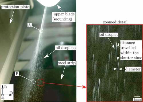
From this bitmap picture, lengths can be approximately measured by counting of pixels. These pixel lengths are then converted into physical lengths using a scaling factor that is determined based on pixel sizes of known objects seen in the photo.

In this way, the droplet diameter can be evaluated with an accuracy of $1.5$ px. For the calculation of the absolute velocity of a droplet, the distance it travels in the photo is divided by the shutter time. The latter is subject to an uncertainty of $20\mathrm{\%}$. The perspective error can be neglected compared to the mentioned uncertainties.

The absolute velocity and the droplet radius of the droplets crossing the positions A (at $25\mathrm{\%}$ of the distance between the blade and the steel strip) and B (at $75\mathrm{\%}$ of the distance between the blade and the steel strip) as indicated for the upper blade in Figure 6 are measured. Since the mentioned measurements are relatively inaccurate, they are performed several times and averaged to get more accurate values. In the following, all the presented measured droplet radii and velocities are average values. These measurements are conducted for different operating conditions at the upper and the lower blade.

The radius $r_0$ of the droplets right after atomization is also measured based on photos. It was found that the oil is not instantaneously atomized right at the blade edge. Instead oil cones, also known as Taylor cones [24], are formed by the electrostatic force and the surface tension acting on the charged oil. If the electrostatic force exceeds the surface tension, oil jets leave the oil cones at their tips and break up into droplets with radius $r_0$ on average (see Figure 7). This effect is used in a broad range of industrial applications including electrohydrodynamic printing [25], electrical discharge machining [26], and minimum quantity lubrication [27] and is described in more detail, e.g. in [24,28–30].

Figure 7. Atomization process at the blade edge (detail from Figure 2(b)).

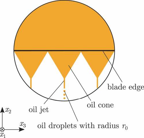
Modelling of this atomization process is complex and entails considerable computational effort. It is therefore omitted here. Instead, $r_0$ is measured and used as an additional input parameter of the model (cf. Figure 4).

It would also be possible to additionally measure the inclination of the droplet trajectories and to use this information for the parameter identification. This was tested but did not further improve the results.

For safety reasons, experimental measurements at the EOM can only be taken for a stationary steel strip, i.e. $v_{strip}=0$. Therefore, the influence of the movement of the strip on the oiling process is studied in simulations as it will be shown in Section 5.

4.2. Parameter identification

A certain part of the measurements, which cover the typical range of operating conditions, is now used to identify the unknown model parameters, i.e. the droplet shape factor $\psi$ in (11), the critical Weber number $W{e}_c$ in (17), and the constant $\kappa$ in (18). These parameters are summarized in the vector $\mathbf{p}=[\psi ,W{e}_c,\kappa {]}^{\mathrm{T}}$ and estimated by minimizing the differences between simulation results and measurements. For this purpose, simulation results and measurements from the six operating scenarios defined in Table 1 are used. The simulation results and measurements are summarized in the vectors ${\mathbf{s}}_n=[u_{A,s},u_{B,s},r_{A,s},r_{B,s}{]}^{\mathrm{T}}$ and ${\mathbf{m}}_n=[u_{A,m},u_{B,m},r_{A,m},r_{B,m}{]}^{\mathrm{T}}$, respectively. The index $n$ defines the operating scenario (see Tab. 0). Here, $u_A$ and $u_B$ are the absolute velocities of the droplets and $r_A$ and $r_B$ are the droplet radii, at the positions A and B, respectively (cf. Figure 6).

Table 1. Operating points for the parameter identification, $v_{strip}=0\mathrm{m}{\mathrm{s}}^{-1}$, $l_u=305\mathrm{m}\mathrm{m}$, and $l_l=135\mathrm{m}\mathrm{m}$.

$n$	$U$ (kV)	$I$ ($\mu$ A)	$Q$ (gs ${ }^{-1}$)	$r_0$ (μm)
Upper Blade
1	30	15	4.7	160
2	60	25	6.8	120
3	90	33	5.6	80
Lower Blade
4	−30	−20	5.1	170
5	−60	−27	6.8	145
6	−90	−55	8.5	110

The optimization problem is formulated as

(21) $\underset{\mathbf{p}\in \mathrm{I}{\mathrm{R}}^3}{min}\sum _{n=1}^6\sum _{k=1}^4\left|\frac{s_{n,k}(\mathbf{p})-m_{n,k}}{m_{n,k}}\right|$(21)

$\mathrm{s}.\mathrm{t}.0<p_1\le 1$

$p_2\ge 0$

$p_3\ge 0$

$\mathrm{A}\mathrm{N}\mathrm{S}\mathrm{Y}\mathrm{S}\mathrm{F}\mathrm{l}\mathrm{u}\mathrm{e}\mathrm{n}\mathrm{t}\mathrm{m}\mathrm{o}\mathrm{d}\mathrm{e}\mathrm{l}\mathrm{o}\mathrm{u}\mathrm{t}\mathrm{l}\mathrm{i}\mathrm{n}\mathrm{e}\mathrm{d}\mathrm{i}\mathrm{n}\mathrm{F}\mathrm{i}\mathrm{g}.5,$

where $s_{n,k}$ and $m_{n,k}$ are the component $k$ of the vectors ${\mathbf{s}}_n$ and ${\mathbf{m}}_n$, respectively. The objective function in (21) is the sum of the normalized absolute differences between the simulated and the measured values for the considered operating points. The problem (21) is solved using the fminsearch-function of the Optimization Toolbox of Matlab. This yields the optimized parameters

(22) ${\mathbf{p}}_{opt}=[0.66,0.24,2.05{]}^{\mathrm{T}}$(22)

4.3. Model validation

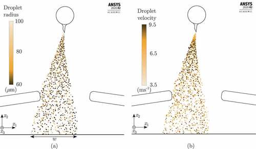
The optimized parameter values (22) are now used to simulate the oiling process for operating points different from the operating conditions used for the parameter identification. Figures 8(a) and figure 8(b) show simulated droplet radii and velocities, respectively, at the upper blade.

Figure 8. Simulation results for $U=75\mathrm{k}\mathrm{V},I=29\mu \mathrm{A},Q=6.8\mathrm{g}{\mathrm{s}}^{-1}$, $r_0=95\mu \mathrm{m}$, $v_{strip}=0\mathrm{m}{\mathrm{s}}^{-1}$, and $l_u=305\mathrm{m}\mathrm{m}$. (a) Droplet radii. (b) Droplet velocities.

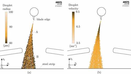
The droplets are injected at the blade edge with the initial radius $r_0$. They are then accelerated and broken up into smaller droplets. Figure 8(b) indicates a strong acceleration of the droplets near the blade edge due to a high electrostatic force and a low drag force acting on the droplets. Their (simulated) values normalized with respect to the droplet mass are given in Table 2 for three representative points.

Table 2. Comparison of (simulated) forces per unit mass acting on the droplets, positions defined in Figure 8(a).

Position	Electrostatic force	Drag force
	($Nk{g}^{-1}$)	($Nk{g}^{-1}$)
Blade edge	$5.4\cdot {10}^4$	$1.5\cdot {10}^{-1}$
A	$1.7\cdot {10}^3$	$2.1\cdot {10}^3$
B	$8.5\cdot {10}^2$	$8.9\cdot {10}^2$

The maximum speed is reached at about $10\mathrm{\%}$ of the distance between the blade and the strip. Afterwards, the droplet velocity decreases due to the decreasing electrostatic force opposed by the drag force which decelerates the droplets (see Table 2, position A).

At position B, the electrostatic force and the drag force are nearly equal and consequently the droplet velocity is almost constant at this point. This can also be inferred from Figure 8(b). The gravitational acceleration $9.81\mathrm{N}\mathrm{k}{\mathrm{g}}^{-1}$ is significantly smaller than the other forces per unit mass acting on the droplets (see Table 2). Its influence on the droplet trajectories is thus negligible.

Table 3 compares some measured and simulated absolute droplet velocities and droplet radii (average values) at the positions A and B and for different operating conditions, used for the model validation. The simulation results are in good agreement with the measured values.

Table 3. Comparison of measured and simulated absolute (mean) droplet velocities $u_A$, $u_B$ and (mean) droplet radii $r_A$, $r_B$ at the positions A and B, respectively, $v_{strip}=0\mathrm{m}{\mathrm{s}}^{-1}$, $l_u=305\mathrm{m}\mathrm{m}$, and $l_l=135\mathrm{m}\mathrm{m}$.

Quantity	Measured	Simulated	Relative error (%)	Conditions
Upper blade
$u_A$ (m/s)	$7.3$	$7.6$	4.1	$U=50\mathrm{k}\mathrm{V}$
$u_B$ (m/s)	$6.4$	$6.7$	4.7	$I=23\mu \mathrm{A}$
$r_A$ (μm)	$90$	$94$	4.4	$Q=6.5\mathrm{g}{\mathrm{s}}^{-1}$
$r_B$ (μm)	$75$	$72$	−4.0	$r_0=140\mu \mathrm{m}$
$u_A$ (m/s)	$9.3$	$9.0$	−3.2	$U=75\mathrm{k}\mathrm{V}$
$u_B$ (m/s)	$8.3$	$7.9$	−4.8	$I=29\mu \mathrm{A}$
$r_A$ (μm)	$70$	$72$	2.9	$Q=6.8\mathrm{g}{\mathrm{s}}^{-1}$
$r_B$ (μm)	$60$	$65$	8.3	$r_0=95\mu \mathrm{m}$
Lower blade
$u_A$ (m/s)	$7.7$	$8.1$	5.2	$U=-50\mathrm{k}\mathrm{V}$
$u_B$ (m/s)	$6.8$	$7.4$	8.8	$I=-20\mu \mathrm{A}$
$r_A$ (μm)	$65$	$62$	−4.6	$Q=4.1\mathrm{g}{\mathrm{s}}^{-1}$
$r_B$ (μm)	$55$	$49$	−10.9	$r_0=150\mu \mathrm{m}$
$u_A$ (m/s)	$8.6$	$9.2$	7.0	$U=-75\mathrm{k}\mathrm{V}$
$u_B$ (m/s)	$7.4$	$7.8$	5.4	$I=-52\mu \mathrm{A}$
$r_A$ (μm)	$45$	$49$	8.9	$Q=9.3\mathrm{g}{\mathrm{s}}^{-1}$
$r_B$ (μm)	$40$	$45$	12.5	$r_0=125\mu \mathrm{m}$

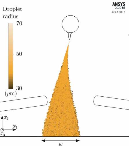
Figure 9 shows the simulated oil spray based on the same operating conditions as in Figure 8 but without the break-up model, i.e. the droplet radius remains constant during the whole simulation.

Figure 9. Simulation results without a break-up model for $U=75\mathrm{k}\mathrm{V},I=29\mu \mathrm{A},Q=6.8\mathrm{g}{\mathrm{s}}^{-1}$, $r_0=62\dots 95\mu \mathrm{m}$, $v_{strip}=0\mathrm{m}{\mathrm{s}}^{-1}$, and $l_u=305\mathrm{m}\mathrm{m}$. (a) Droplet radii. (b) Droplet velocities.

In contrast to Figure 8, the initial droplet radius $r_0$ is not the same for all the droplets but is distributed between $62\mu$ m and $95\mu$ m (the same range as in 8(a) under consideration of the droplet break-ups). This corresponds to the standard approach used in the literature, see, e.g. [3–5]. The oil spray width $w$ in Figure 9 is clearly larger than in Figure 8 and the droplet radii and velocities summarized in Table4 differ from the simulated (with break-up model) and measured values shown in Table 3.

Table 4. Simulated absolute (mean) droplet velocities $u_A$, $u_B$ and (mean) droplet radii $r_A$, $r_B$ at the positions A and B, respectively, without a break-up model and $v_{strip}=0\mathrm{m}{\mathrm{s}}^{-1}$, $l_u=305\mathrm{m}\mathrm{m}$, and $l_l=135\mathrm{m}\mathrm{m}$.

Quantity	Simulated	Conditions
Upper blade
$u_A$ (m/s)	$8.5$	$U=75\mathrm{k}\mathrm{V}$
$u_B$ (m/s)	$7.0$	$I=29\mu \mathrm{A}$
$r_A$ (μm)	$79$	$Q=6.8\mathrm{g}{\mathrm{s}}^{-1}$
$r_B$ (μm)	$79$	$r_0=62\dots 95\mu \mathrm{m}$

The calculation time without the break-up model is 56s (for the same convergence criterion). This is only slightly shorter than the calculation time of the full model with the break-up submodel included.

4.4. Plausibility check using the Rayleigh limit

Equation (15)(15) $r_R={\left(\frac{{\rho }_{d}I}{6QK\sqrt{{\in }_0\gamma }}\right)}^{-\frac{2}{3}}$(15) , which follows from the Rayleigh limit (13), defines the maximum stable droplet radius $r_R$ for a given charge to mass ratio $\frac{I}{Q}$. This means that the radii of all child droplets must not exceed this limit after the break-up process. This must be satisfied for a scaling factor $K$ in (15) within a subset of $[0.55,0.8]$ according to [15]. It turns out that in our case this holds true for $K\in [0.7,0.8]$. Table 5 compares the radii limits calculated based on (15) with the measured and simulated droplet radii at the position B for $K=0.7$. It is assumed that the droplets do not break up any further after crossing position B because the droplet velocities continuously decrease below position A (cf. Figure 8(b)). In accordance with the theory, all measured and simulated droplet radii are below $r_R$.

Table 5. Comparison of calculated droplet radius limits $r_R$ according to (15) (for K = 0.7) with measured and simulated (mean) droplet radii at position B, $v_{strip}=0\mathrm{m}{\mathrm{s}}^{-1}$, $l_u=305\mathrm{m}\mathrm{m}$, and $l_l=135\mathrm{m}\mathrm{m}$.

$r_R$	$r_B$	$r_B$
($\mu$ m)	Measured	Simulated	Conditions
	(μm)	(μm)
Upper blade
			$U=50$ kV
77	75	72	$I=23\mu$ A
			$Q=6.5\mathrm{g}{\mathrm{s}}^{-1}$
			$r_0=140\mu$ m
			$U=75$ kV
67	60	65	$I=29\mu$ A
			$Q=6.8\mathrm{g}{\mathrm{s}}^{-1}$
			$r_0=95\mu$ m
Lower blade
			$U=-50$ kV
61	55	49	$I=-20\mu$ A
			$Q=4.1\mathrm{g}{\mathrm{s}}^{-1}$
			$r_0=150\mu$ m
			$U=-75$ kV
56	40	45	$I=-52\mu$ A
			$Q=9.3\mathrm{g}{\mathrm{s}}^{-1}$
			$r_0=125\mu$ m

5. Simulation results and sensitivity analysis

The validated model can be used in simulations to obtain valuable process insights. For example, Figure 10 presents the simulated electric field strength.

Figure 10. Simulated electric field strength (log scale) for $U=75\mathrm{k}\mathrm{V},I=29\mu \mathrm{A},Q=6.8\mathrm{g}{\mathrm{s}}^{-1}$, $r_0=95\mu \mathrm{m}$, $v_{strip}=0\mathrm{m}{\mathrm{s}}^{-1}$, and $l_u=305\mathrm{m}\mathrm{m}$.

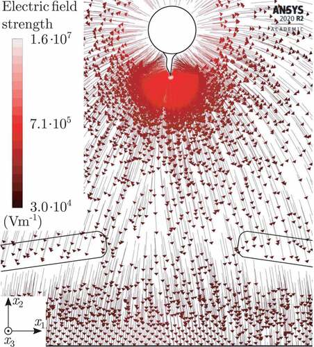
Its maximum is near the blade edge, which is why the atomization of the oil takes place at this position. As can be inferred from Figure 8, the oil spray is not symmetric with respect to the vertical centerplane of the EOM. The asymmetry of the oil spray roots in the asymmetric geometry of the oiling blade and the resulting asymmetric electric field.

The validated model is also used to analyse and better understand the dependence of output variables like the droplet radius $r$, the absolute droplet velocity $u$, the charge $q$ carried by the droplets, the travel time $t_{bs}$ of the droplets from the blade to the strip, the spray width $w$, and the absolute airflow velocity $v$ on the input variables, i.e. the voltage $U$, the oil mass flow rate $Q$, and the strip velocity $v_{strip}$. For example, Figure 11 shows the oil spray for a voltage of $U=100$ kV, which is higher than in all scenarios considered so far.

Figure 11. Simulated droplet radii for $U=100\mathrm{k}\mathrm{V},I=36\mu \mathrm{A},Q=6.8\mathrm{g}{\mathrm{s}}^{-1}$, $r_0=70\mu \mathrm{m}$, $v_{strip}=0\mathrm{m}{\mathrm{s}}^{-1}$, and $l_u=305\mathrm{m}\mathrm{m}$.

A comparison with Figure 8(a) reveals that the droplet radii decrease and the oil spray width $w$ increases with increasing voltage. The physical reason behind this observations is an increased charge carried by the droplets. Consequently, the droplets break up into smaller droplets and the repulsion between them is higher.

As already mentioned in Section 4.1, for safety reasons, experimental measurements at the EOM can only be taken for $v_{strip}=0$, and therefore the influence of the movement of the strip on the oiling process is studied in simulations. Figure 12(a) shows the simulated absolute airflow velocity induced by the movement of the oil droplets and the steel strip, which travels with $v_{strip}=5\mathrm{m}{\mathrm{s}}^{-1}$.

Figure 12. Simulation results for $U=75\mathrm{k}\mathrm{V},I=29\mu \mathrm{A},Q=6.8\mathrm{g}{\mathrm{s}}^{-1}$, $r_0=95\mu \mathrm{m}$, $v_{strip}=5\mathrm{m}{\mathrm{s}}^{-1}$, and $l_u=305\mathrm{m}\mathrm{m}$. (a) Air flow velocity. (b) Droplet velocities.

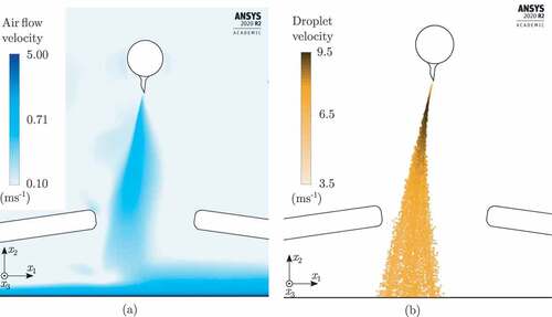
Because of the no-slip boundary condition at the steel strip, the airflow velocity approaches $v_{strip}$ in the vicinity of the steel strip.

Figure 12(b) presents the simulated droplet velocities for $v_{strip}=5\mathrm{m}{\mathrm{s}}^{-1}$. A comparison between Figures 12(b) and 8(b) indicates that there is no significant influence of the airflow induced by the movement of the strip on the droplet trajectories. This is because of the high velocity and inertia of the droplets and the low thickness of the airflow boundary layer at the strip surface.

Table 6 summarizes the qualitative dependencies between the input and output variables found in simulations and measurements.

Table 6. Dependence of the output variables on the input variables.

Input	Output
	$r$	$u$	$q$	$t_{bs}$	$w$	$v$
$U\uparrow$	$\downarrow$	$\uparrow$	$\uparrow$	$\downarrow$	$\uparrow$	$\uparrow$
$Q\uparrow$	$\simeq$	$\simeq$	$\simeq$	$\uparrow$	$\uparrow$	$\uparrow$
$v_{strip}\uparrow$	$\simeq$	$\simeq$	$\simeq$	$\simeq$	$\simeq$	$\uparrow$

6. Case study: model-based optimization of the angular blade orientation

This section deals with the negative effect of a laterally inclined oiling blade on the oil distribution at the strip surface. Measurements revealed that even a very small lateral inclination $d$ of the upper oiling blade (see Figure 13) can lead to highly undesired laterally non-uniform oil distribution.

Figure 13. Laterally inclined upper blade.

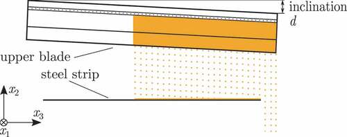
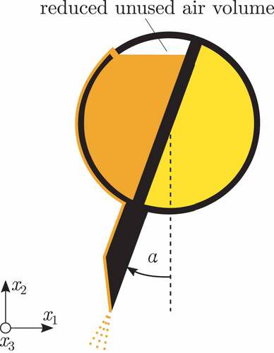
In the current design of the mountings of the oiling blades, it is a difficult task to adjust the oiling blades and a lateral inclination cannot be entirely prevented. It was found that an unused air volume remains above the nozzles in the cavity of the upper blade as depicted in Figure 3. Due to gravity, the air accumulates at the elevated side of the inclined blade, which is why more oil leaves the cavity through the nozzles at the lower side. A rotation of the upper blade by the angle $\alpha$ defined in Figure 14 reduces the unused air volume, as a comparison between Figures 14 and 3 clarifies.

Figure 14. Reduced unused air volume in the rotated upper blade.

In practical experiments, it was found that this change also reduces the dependence of the oil distribution on the lateral inclination $d$ of the blade. However, there is an upper limit for the angle $\alpha$ to avoid that the oil spray hits the protection plates of the EOM. To avoid time-consuming manual optimization of $\alpha$ by trial and error, the optimum angle $\alpha$ is determined in simulations using the developed mathematical model. Figure 15 shows the simulated oil spray for the maximum angle ${\alpha }_{max}={20}^{\circ }$ for the operating conditions $U=50\mathrm{k}\mathrm{V}$, $I=25\mu \mathrm{A}$, $Q=6.1\mathrm{g}{\mathrm{s}}^{-1}$, $r_0=95\mu \mathrm{m}$, $v_{strip}=5\mathrm{m}{\mathrm{s}}^{-1}$, and $l_u=305\mathrm{m}\mathrm{m}$.

Figure 15. Simulated droplet radii for $U=50\mathrm{k}\mathrm{V}$, $I=25\mu \mathrm{A}$, $Q=6.1\mathrm{g}{\mathrm{s}}^{-1}$, $r_0=135\mu \mathrm{m}$, $v_{strip}=5\mathrm{m}{\mathrm{s}}^{-1}$, $l_u=305\mathrm{m}\mathrm{m}$, and $\alpha ={20}^{\circ }$.

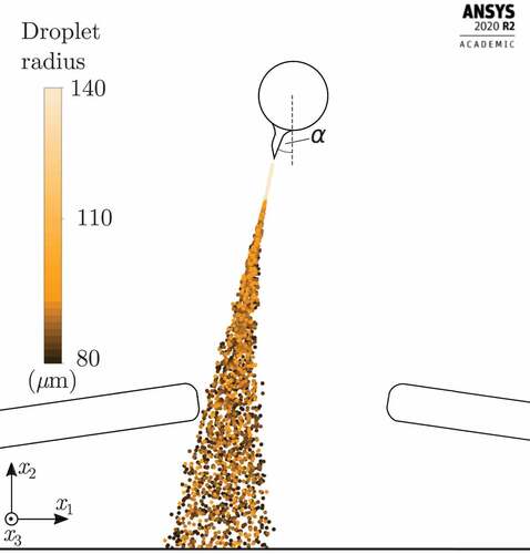
This application of the presented model demonstrates that the consideration of the break-up of the droplets (see difference between Figures 8(a) and 9(a)) is necessary to get valid results.

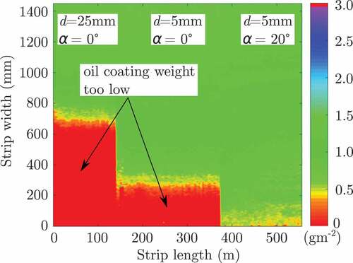
The optimized angle ${\alpha }_{max}={20}^{\circ }$ was then tested at the real plant. From this test scenario, Figure 16 shows the measured oil distribution (coating weight) on the strip for two different inclinations $d$ and angular blade orientations $\alpha$. The permissible range of the oil film thickness is shown in green. This measurement confirms an improvement of the oil distribution by optimizing the angle $\alpha$.

Figure 16. Measured oil coating weight on the upper strip surface for $U=50\mathrm{k}\mathrm{V}$, $I=29\mu \mathrm{A}$, $Q=6.5\mathrm{g}{\mathrm{s}}^{-1}$, $r_0=135\mu \mathrm{m}$, $v_{strip}=5\mathrm{m}{\mathrm{s}}^{-1}$, and $l_u=305\mathrm{m}\mathrm{m}$.

7. Conclusions

In this paper, an experimentally validated mathematical model of the electrostatic spraying process in an industrial electrostatic oiling machine (EOM) for steel strips was presented. Electrostatic oiling is a complex, nonlinear multiphysics problem with a two-phase fluid flow and distributed parameters. A numerical, two-dimensional, two-phase, steady-state model of a specific EOM is developed that allows for the simulation and optimization of the oiling process regarding the uniformity of the oil film thickness. In contrast to other works in this area, a secondary break-up submodel is included that describes the break-up of the oil droplets induced by the drag force and repelling forces between the charges carried by them. Consideration of the droplet break-ups in the model increases the accuracy of the calculated droplet trajectories and is necessary to get valid simulation results, which are used for an optimization of the oiling process. The simulation results of the developed mathematical model show a good agreement with data measured at a real industrial EOM. Furthermore, only one set of model parameters is needed for the considered range of operating conditions. In addition, the simulated droplet diameters match the theoretical predictions based on the Rayleigh limit.

The simulations and measurements show that the droplet velocities increase with increasing blade voltages and that the droplets carry more charge with increasing voltage. As a consequence, the droplets break up into smaller droplets and the oil spray is widened. The simulations show that the electric field is more than ten times higher at the blade edge than at other positions on the blade surface or below it. This is why the atomization of the oil takes place directly at the blade edge. Also the orientation of the oil spray depends on the blade geometry. Moreover, it was shown that the droplet trajectories are hardly influenced by the gravitational force, but mainly defined by the electrostatic force and the drag force.

The airflow induced by the strip movement was found to have only a small influence on the oil spray. In fact, this influence is limited to the boundary layer right on the strip surface.

The validated model can be also used to study the dependence of the output variables, i.e. the droplet radius $r$, the absolute droplet velocity $u$, the charge $q$ carried by the droplets, the droplet travel time $t_{bs}$ from the blade to the strip, the spray width $w$, and the absolute airflow velocity $v$ on the input variables, i.e. the voltage $U$, the oil mass flow rate $Q$, and the strip velocity $v_{strip}$.

In practical experiments, it was found that a laterally inclined upper blade leads to a non-uniform oil distribution on the strip. This is because of air which remains in the cavity of the blade above the nozzles. Excess air accumulates at the elevated side of the blade. An optimization of the angular blade orientation with respect to its lateral axis reduces this effect and improves the oil film distribution on the strip. In this context, the simulation model was successfully used to determine the optimum angular blade orientation.

The presented model does not include the charging and atomization process of the oil at the blade edge. Hence, the radius of the droplets right after the atomization $r_0$ and the current $I$ are additional input parameters of the model and have to be measured. An extension to calculate $r_0$ and $I$ as functions of the voltage, the oil mass flow rate, the blade geometry, and other operating parameters, or the use of look-up tables for the relations would lead to a stand-alone simulation model, and may be the focus of a future work.

Acknowledgments

The financial support by the Austrian Federal Ministry for Digital and Economic Affairs, the National Foundation for Research, Technology and Development and the Christian Doppler Research Association, and voestalpine Stahl GmbH is gratefully acknowledged.

Disclosure statement

No potential conflict of interest was reported by the author(s).

Additional information

Funding

This work was supported by the Austrian Federal Ministry for Digital and Economic Affairs, the National Foundation for Research, Technology and Development, the Christian Doppler Research Association, and voestalpine Stahl GmbH. The authors acknowledge TU Wien Bibliothek for financial support through its Open Access Funding Programme.

References

- L. Jadachowski, A. Steinboeck, and A. Kugi, Two-dimensional thermal modelling with specular reflections in an experimental annealing furnace, Math Comput Model Dyn Syst 23 (2017), pp. 23–39.
- K.R. Ellwood and J. Braslaw, A finite-element model for an electrostatic bell sprayer, J. Electrost. 45 (1998), pp. 1–23. doi:10.1016/S0304-3886(98)00011-4.
- Q. Ye and J. Domnick, On the simulation of space charge in electrostatic powder coating with a Corona spray gun, Powder Technol. 135-136 (2003), pp. 250–260. doi:10.1016/j.powtec.2003.08.019.
- N. Toljic, K. Adamiak, G. Castle, H.H. Kuo, and H.T. Fan, A full 3D numerical model of the industrial electrostatic coating process for moving targets, J. Electrost. 71 (2013), pp. 299–304. doi:10.1016/j.elstat.2012.12.032.
- Q. Ye and J. Domnick, Analysis of droplet impingement of different atomizers used in spray coating processes, J. Coat. Technol Res. 14 (2017), pp. 467–476. doi:10.1007/s11998-016-9867-4.
- S. Zhao, K. Adamiak, and G.S.P. Castle , The implementation of Poisson field analysis within Fluent to model electrostatic spraying, Proc. Can. Conf. Electr. Comput. Eng. 5 (2007), pp. 1456–1459.
- J.D. Jackson, Classical Electrodynamics, 3rd ed., Wiley, New York, 1998.
- D.J. Acheson, Elementary Fluid Dynamics. Oxford, UK: Oxford University Press, 1990.
- A.D. Gosman and E. Ioannides, Aspects of computer simulation of liquid-fuelled combustors, J. Energy 7 (1983), pp. 482–490. doi:10.2514/3.62687.
- A. Haider and O. Levenspiel, Drag coefficient and terminal velocity of spherical and nonspherical particles, Powder Technol. 58 (1989), pp. 63–70. doi:10.1016/0032-5910(89)80008-7.
- J.W.S. Rayleigh, On the equilibrium of liquid conducting masses charged with electricity, London Edinburgh Dublin Phil. Mag. J. Sci. 14 (1882), pp. 184–186. doi:10.1080/14786448208628425.
- B. Chen, D. Gao, Y. Li, C. Chen, X. Yuan, Z. Wang, and P. Sun, Investigation of the droplet characteristics and size distribution during the collaborative atomization process of a twin-fluid nozzle, Int. J. Adv. Manuf. Technol. 107 (3–4) (2020), pp. 1625–1639. doi:10.1007/s00170-020-05131-1.
- A. Gomez and K. Tang, Charge and fission of droplets in electrostatic sprays, Phys. Fluids 6 (1) (1994), pp. 404–414. doi:10.1063/1.868037.
- L. de Juan and J. Fernández de la Mora, Charge and size descriptions of electrospray drops, J. Colloid Interface Sci. 186 (1997), pp. 280–293. doi:10.1006/jcis.1996.4654.
- J. Shrimpton, Dielectric charged drop break-up at sub-Rayleigh limit conditions, IEEE Trans. Dielectr. Electr. Insul. 12 (2005), pp. 573–578. doi:10.1109/TDEI.2005.1453462.
- P. O’Rourke and A. Amsden, The TAB method for numerical calculation of spray droplet breakup, SAE Tech. Pap. 872089 (1987), pp. 1–10.
- R.D. Reitz, Mechanisms of atomization processes in high-pressure vaporizing sprays, At. Sprays. Technol. 3 (1987), pp. 309–337.
- J.C. Beale and R.D. Reitz, Modeling spray atomization with the Kelvin-Helmholtz/Rayleigh-Taylor hybrid model, At. Sprays 9 (1999), pp. 623–650. doi:10.1615/AtomizSpr.v9.i6.40.
- S.V. Apte, M. Gorokhovski, and P. Moin, LES of atomizing spray with stochastic modeling of secondary breakup, Int. J. Multiph. Flow. 29 (9) (2003), pp. 1503–1522. doi:10.1016/S0301-9322(03)00111-3.
- P. Day, A. Manz, and Y. Zhang, Microdroplet Technology: Principles and Emerging Applications in Biology and Chemistry. Berlin: Springer, 2012.
- H. Taghavifar, S. Khalilarya, S. Jafarmadar, and F. Baghery, 3-D numerical consideration of nozzle structure on combustion and emission characteristics of DI diesel injector, Appl. Math. Model. 40 (19–20) (2016), pp. 8630–8646. doi:10.1016/j.apm.2016.05.010.
- B.E. Launder and D.B. Spalding, Lectures in mathematical models of turbulence. London, New York: Academic Press. 1972.
- T. Shih, W. Liou, A. Shabbir, and J. Zhu, A new k – ε eddy-viscosity model for high Reynolds number turbulent flows - model development and validation, Comput. Fluids 24 (1995), pp. 227–238. doi:10.1016/0045-7930(94)00032-T.
- A. Bailey, Electrostatic spraying of liquids, Phys. Bull. 35 (4) (1984), pp. 146–148. doi:10.1088/0031-9112/35/4/018.
- M.A.A. Rehmani and K.M. Arif, High resolution electrohydrodynamic printing of conductive ink with an aligned aperture coaxial printhead, Int. J. Adv. Manuf. Technol. 115 (2021), pp. 2785–2800. doi:10.1007/s00170-021-07075-6.
- Y. Zhang, N. Han, X. Kang, K. Wilt, W. Zhao, and J. Ni, The tool electrode investigation of electrostatic field-induced electrolyte jet (e-jet) electrical discharge machining, Int. J. Adv. Manuf. Technol. 82 (5–8) (2016), pp. 1455–1461. doi:10.1007/s00170-015-7911-7.
- Y. Su, H. Jiang, and Z. Liu, A study on environment-friendly machining of titanium alloy via composite electrostatic spraying, Int. J. Adv. Manuf. Technol. 110 (5–6) (2020), pp. 1305–1317. doi:10.1007/s00170-020-05925-3.
- K.S. Robinson and R.J. Turnbull, Electrostatic spraying of liquid insulators, IEEE Trans. Ind. Appl. IA-16 (2) (1980), pp. 308–317. doi:10.1109/TIA.1980.4503787.
- A. Jaworek and A. Krupa, Classification of the modes of EHD spraying, J Aerosol Sci 30 (7) (1999), pp. 873–893. doi:10.1016/S0021-8502(98)00787-3.
- O. Lastow and W. Balachandran, Numerical simulation of electrohydrodynamic (EHD) atomization, J. Electrost. 64 (12) (2006), pp. 850–859. doi:10.1016/j.elstat.2006.02.006.