Towards real-time fluid dynamics simulation: a data-driven NN-MPS method and its implementation

ABSTRACT

In this work, we construct a data-driven model to address the computing performance problem of the moving particle semi-implicit method by combining the physics intuition of the method with a machine-learning algorithm. A fully connected artificial neural network is implemented to solve the pressure Poisson equation, which is reformulated as a regression problem. We design context-based feature vectors for particle-based on the Poisson equation. The neural network maintains the original particle method’s accuracy and stability, while drastically accelerates the pressure calculation. It is very suitable for GPU parallelization, edge computing scenarios and real-time simulations.

KEYWORDS:

• Data-driven
• Lagrangian particle method
• edge computing

1. Introduction

The moving particle semi-implicit (MPS) method, initially proposed by Koshizuka and Oka [1], was developed to solve the Navier–Stokes equations in the Lagrangian framework for incompressible viscous flows. It is essentially a fractional step method that consists of the split of each time step into two steps of prediction and the correction. The MPS method improves the accuracy and stability of the pressure calculation compared to many other particle methods that calculate pressure explicitly, like the smooth particle hydrodynamics (SPH) [2]. Giving the stability of the pressure calculation and the convenience of dealing with free-surface boundary conditions, MPS are widely implemented to address problems like haemodynamics simulations [3], large-scale simulations on geographical phenomena [4] and analysis on material processing [5]. However, accuracy comes at the cost of computational resources and time. In the MPS scheme, the pressure of the next frame is derived from solving the pressure Poisson equation. The preconditioned conjugate gradient (PCG) method or the incomplete Cholesky conjugate gradient (ICCG) method is usually used to solve the discrete pressure Poisson equation and requires enormous computational resources as the number of particles is large. This is also discussed in [6]. Generally speaking, these iterative methods are not suitable for the GPU parallelization. Hence, large-scale simulations using MPS are difficult without high-performance CPU clusters; it prohibits MPS from being widely employed as a desktop tool for engineers. A modified method, the explicit MPS method [7], has been proposed to make the solving process more suitable for the GPU parallelization and to reduce the computational cost. It calculates the pressure explicitly; the calculation of each particle is independent and, thus, can be carried out on different threads simultaneously. However, the explicit calculation mode is susceptible to the time step value and is less stable compared to the implicit mode.

With excellent computing power (especially in GPU) and sophisticated AI hardware technologies, data-driven methods are now gaining more and more attention. In areas like computer vision, natural language processing and machine learning, they have been proven to be very effective. Apart from these well-known implementations, machine learning can also be employed to address the physics problem. Many data-driven models are used in fluid dynamics where most of them manage to reduce the computational cost. A common idea is the model reduction techniques, for example see [8–12]. They project the Navier–Stokes equations into the low-dimensional space. With a decrease in the representation completeness, they can bring considerable speed-up to the problem. For Lagrangian particle fluid simulations, the random forest technique [13] is implemented to predict each particle’s acceleration with a context-based feature vector as the input. It does not require an iterative solver and attains a real-time calculation speed. In [14], an efficient and lightweight cheap neural network architecture is used to predict fluid dynamics and to generate realistic animations. In [15], the physics-informed neural network (PINN) is used for the neural particle method. For Eulerian grid-based simulations, neural networks [16] and convolutional neural networks [17] have been implemented to replace traditional pressure projection methods. These data-driven methods significantly reduce the computational cost, produce a realistic fluid-like effect and shed light on building high-fidelity data-driven models for fluid simulations. We are interested in gaining the physics intuition from MPS such that the constructed data-driven model can accelerate the calculation, save computational resources, and generate reliable results for engineering problems.

In this paper, we employ an artificial neural network (NN) to address the computational cost problem in the original MPS method. We reformulate the pressure Poisson equation as a regression problem depending on the context-based feature vector we designed. The training data are generated using the original MPS method with a conjugate gradient (CG) solver. The MPS method with a neural network (NN-MPS) we proposed can significantly improve the efficiency of the pressure calculation as it is free of iterations used, for example, in the CG method. Also, the calculation of each particle is independent; the computation can be easily parallelized. We compare the performance of NN-MPS and MPS using a dam collapse problem with experimental results from Martin and Moyce [18], which demonstrates the accuracy of NN-MPS. We also test NN-MPS on several other scenes. These results show that NN-MPS has a robust performance and can significantly improve the calculation speed. At the same time, we also deploy NN-MPS on edge computing devices with AI chips to verify the possibility of achieving higher performance on AI devices and to demonstrate its potential for real-time applications.

2. Moving particle semi-implicit method

2.1. Governing equation

In the MPS scheme, the governing equations for incompressible viscous flow simulations are the continuity and the Navier–Stokes equations:

$\begin{array}{rl}& \frac{D\rho }{Dt}=0,\\ & \frac{D\mathit{u}}{Dt}=-\frac{\mathrm{\nabla }p}{\rho }+\nu {\mathrm{\nabla }}^2\mathit{u}+\mathit{g},\end{array}$

where $\frac{D}{Dt}$ is the material derivative for time, $u$ is velocity, $g$ is the external body force per unit mass, $\rho$ and $\nu$ are the density and kinematic viscosity, respectively.

2.2. Kernel function and particle number density

The kernel function describes how a particle interacts with others in its vicinity. In this work, we adopt the same kernel function from the original MPS method, see [1]. The radius of the interaction area is determined by the parameter $r_e$,

$w(r)=\left\{\begin{array}{cc}\frac{r_e}{r}-1,& (0\le r<r_e)\\ 0& (r_e\le r)\end{array}\right..$

Particle number density at coordinate $r_i$, where the particle $i$ is located, is defined by

$N_i=\sum _{j\ne i}w(|{\mathit{r}}_j-{\mathit{r}}_i|).$

If the incompressible condition is satisfied, the particle number density should be constant $N^0$.

2.3. Discrete differential operators

A gradient vector between two particles $i$ and $j$ having scalar quantities ${\varphi }_i$ and ${\varphi }_j$ at coordinates ${\mathit{r}}_i$ and ${\mathit{r}}_j$ is defined [1] as

${⟨\mathrm{\nabla }\varphi ⟩}_i=\frac{d}{N^0}\sum _{j\ne i}\left[\frac{{\varphi }_j-min({\varphi }_i)}{|{\mathit{r}}_j-{\mathit{r}}_i{|}^2}({\mathit{r}}_j-{\mathit{r}}_i)w(|{\mathit{r}}_j-{\mathit{r}}_i|)\right],$

where $d$ is the dimension of the space, $min({\varphi }_i)$ denotes the minimum value of a scalar quantity $\varphi$ among the neighbouring particles of particle $i$.

Similarly, a divergence scalar quantity between two particles $i$ and $j$ having vector quantities ${\vec{\varphi }}_i$ and ${\vec{\varphi }}_j$ at coordinates ${\mathit{r}}_i$ and ${\mathit{r}}_j$ can be defined as

${⟨\mathrm{\nabla }\cdot \vec{\varphi }⟩}_i=\frac{d}{N^0}\sum _{j\ne i}\left[\frac{{\vec{\varphi }}_j-{\vec{\varphi }}_i}{|{\mathit{r}}_j-{\mathit{r}}_i{|}^2}({\mathit{r}}_j-{\mathit{r}}_i)w(|{\mathit{r}}_j-{\mathit{r}}_i|)\right].$

The Laplacian model is derived from solving a diffusion equation, i.e.

${⟨{\mathrm{\nabla }}^2\varphi ⟩}_i=\frac{2d}{N^0\lambda }\sum _{j\ne i}({\varphi }_j-{\varphi }_i)w(|{\mathit{r}}_j-{\mathit{r}}_i|),$

where the normalization parameter $\lambda$ is given by

$\lambda =\frac{{\int }_{V}w(r)r^{2}dv}{{\int }_{V}w(r)dv},$

where $V$ denotes the neighbourhood of particle $i$.

2.4. Boundary condition and searching neighbour particles

In the MPS method, dynamic boundary conditions are imposed to deal with the free-surface. The particle number density is smaller for particles in the vicinity of free-surface because their neighbourhoods include empty air regions. Particles satisfying the following criteria are considered as on the free-surface.

$N_i^{\ast }<\beta N^0,$

where $\beta$ in this work is selected to be $\beta =0.97$. In the pressure calculation, the dynamic free-surface condition is satisfied by setting the pressure of free-surface particles to be zero, which equals the atmospheric pressure.

For the wall boundary condition, as shown in Figure 1, two layers of wall particles are placed along the solid boundary, surrounded by two layers of ghost particles. For the pressure calculation, the wall particles are used; they interact with nearby fluid particles, while their positions keep stationary. The ghost particles are only taken into consideration for calculating the particle number density to avoid that wall particles are identified to free-surface particles.

Figure 1. The arrangement of particles near the wall.

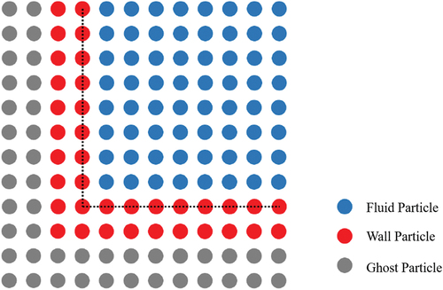
Many steps of the MPS method requires neighbour particles searching. Three searching techniques are commonly used in particle methods. They are the linear scanning, the linked-list searching [7], and the tree searching [19]. In this work, we use the linked-list searching technique. The linked-list searching places a temporary grid on the calculation region, and particles are assigned to different cells. Particles in the same or adjacent cells are considered.

2.5. Velocity update scheme

The MPS method is a predictor-corrector method for the velocity, which includes three main steps [20].

Firstly, it transits particles using viscosity force, body forces, and applies then collision detection.

$\begin{array}{rl}& {\mathit{u}}_{\mathit{i}}^{\mathbf{\ast }}\mathbf{=}{\mathit{u}}_{\mathit{i}}^{\mathit{n}}\mathbf{+}\mathbf{(}\mathit{\nu }{\mathbf{\nabla }}^{\mathbf{2}}{\mathit{u}}^{\mathit{n}}\mathbf{+}\mathit{g}\mathbf{)}\mathbf{\Delta }\mathit{t}\mathbf{,}\\ & {\mathit{r}}_{\mathit{i}}^{\mathbf{\ast }}\mathbf{=}{\mathit{r}}_{\mathit{i}}^{\mathit{n}}\mathbf{+}{\mathit{u}}_{\mathit{i}}^{\mathbf{\ast }}\mathbf{.}\end{array}$

Secondly, it calculates the source term and the coefficient matrix using the temporary location ${\mathit{r}}_i^{\ast }$ and the temporary velocity $u_i^{\ast }$ and solves the pressure Poisson equation. We use the modified source term from Lee et al. [20],

${\mathrm{\nabla }}^2{p}_i^{n+1}=(1-\gamma )\frac{\rho }{\mathrm{\Delta }t}\mathrm{\nabla }\cdot {\mathit{u}}_i^{\ast }+\gamma \frac{\rho }{\mathrm{\Delta }{t}^2}\frac{N^0-N_i^{\ast }}{N^0},$

where ${\mathit{u}}_i^{\ast }$ denotes the temporary velocity of particle $i$, $N_i^{\ast }$ is the temporary particle number density of particle $i$, $\gamma$ is a blending parameter ranging from 0.0 to 1.0. Based on our numerical tests, we set $\gamma =0.2$.

Finally, it uses the predicted pressure $p_i^{n+1}$ to update the temporary velocity ${\mathit{u}}_i^{\ast }$ and temporary location $r_i^{\ast }$, i.e.

$\begin{array}{rl}& {\mathit{u}}_i^{n+1}={\mathit{u}}_i^{\ast }-\frac{\mathrm{\Delta }t}{\rho }\mathrm{\nabla }{p}_i^{n+1},\\ & {\mathit{r}}_i^{n+1}={\mathit{r}}_i^{\ast }+\frac{1}{2}(u_i^{\ast }+u_i^{n+1})\mathrm{\Delta }t.\end{array}$

3. A data driven pressure model

3.1. Modelling of incompressibility using a data-driven pressure projection

In the MPS method, the calculation of pressure uses the continuity equation and the method keeps the particle number density $N^{\ast }$ to be constant $N^0$. The discrete Poisson equation of pressure for particle $i$ is

$p_i=\frac{1}{N_i^{\ast }}\left\{\sum _{j\ne i}\left(p_{j}w(|{\mathit{r}}_j-{\mathit{r}}_j|)\right)-\frac{N^0\lambda }{2d}\left[(1-\gamma )\frac{\rho }{\mathrm{\Delta }t}\mathrm{\nabla }\cdot {\mathit{u}}_i^{\ast }+\gamma \frac{\rho }{\mathrm{\Delta }{t}^2}\frac{N^0-N_i^{\ast }}{N^0}\right]\right\}.$

Since it is based on the interaction between the particle and it neighbour particles, it has to be solved globally (simultaneously for all particles), which brings challenges to the parallelization. Also, for large-scale problems, solving large sparse systems can be expensive. To address this problem, we design a data-driven model to efficiently carry out the pressure calculation while maintaining the robustness and stability. We reformulate the pressure projection step as a data-driven regression problem. The machine learning model used in this work is the neural network. However, it relies on the initialization of weight parameters, and many of its mechanism is still not so well understood. Yet, its capability of extracting, transforming low-level features and fitting nonlinear function makes it an excellent choice to serve as a regressor.

To ensure the robustness and accuracy of the neural network, choosing an appropriate representation for the model’s input is very important. In traditional data-driven modelling problems, techniques like principle components analysis (PCA) are implemented to derive representative feature of the input data. Since the issue addressed here is physics-informed, the construction of the feature vector can be referred to the original MPS method.

In the pressure Poisson equation, we have

$\frac{2d}{N^0\lambda }\left[\sum _{j\ne i}(p_{j}w(|{\mathit{r}}_j-{\mathit{r}}_i|))-p_i\sum _{j\ne i}w(|{\mathit{r}}_j-{\mathit{r}}_i|)\right]=(1-\gamma )\frac{\rho }{\mathrm{\Delta }t}\mathrm{\nabla }\cdot {\mathit{u}}_i^{\ast }+\gamma \frac{\rho }{\mathrm{\Delta }{t}^2}\frac{N^0-N_i^{\ast }}{N^0}.$

And it can be rearranged as

(1) $p_i=\frac{1}{N_i^{\ast }}\left\{\sum _{j\ne i}\left(p_{j}w(|{\mathit{r}}_j-{\mathit{r}}_j|)\right)-\frac{N^0\lambda }{2d}\left[(1-\gamma )\frac{\rho }{\mathrm{\Delta }t}\mathrm{\nabla }\cdot {\mathit{u}}_i^{\ast }+\gamma \frac{\rho }{\mathrm{\Delta }{t}^2}\frac{N^0-N_i^{\ast }}{N^0}.\right]\right\}.$(1)

From equation (1)(1) $p_i=\frac{1}{N_i^{\ast }}\left\{\sum _{j\ne i}\left(p_{j}w(|{\mathit{r}}_j-{\mathit{r}}_j|)\right)-\frac{N^0\lambda }{2d}\left[(1-\gamma )\frac{\rho }{\mathrm{\Delta }t}\mathrm{\nabla }\cdot {\mathit{u}}_i^{\ast }+\gamma \frac{\rho }{\mathrm{\Delta }{t}^2}\frac{N^0-N_i^{\ast }}{N^0}.\right]\right\}.$(1) , the pressure of the centre particle $i$ relies on its temporary velocity and particle number density, and the weighted pressure of other particles in its neighbourhood. Based on this implicit relationship, we consider the regression problem of form

${\hat{p}}^{n+1}=H({\varphi }_i^{\mathrm{p}\mathrm{r}\mathrm{e}\mathrm{s}},{\varphi }_1^{\mathrm{p}\mathrm{r}\mathrm{e}\mathrm{s}},{\varphi }_2^{\mathrm{p}\mathrm{r}\mathrm{e}\mathrm{s}},\cdots ,{\varphi }_n^{\mathrm{p}\mathrm{r}\mathrm{e}\mathrm{s}},N_i^{\ast },\mathrm{\nabla }\cdot {\mathit{u}}_i^{\ast }),$

where $H$ is the neural network regressor that projects the feature vector into the pressure solution space, ${\varphi }_{(\cdot )}$ denotes the integral pressure feature of the centre particle or neighbour particles.

For a centre particle $i$ and particles in its neighbourhood, as shown in Figure 2, the integral pressure feature is defined as

Figure 2. A description of a particle and its neighborhood.

$\begin{array}{rl}& {\varphi }_i^{\mathrm{p}\mathrm{r}\mathrm{e}\mathrm{s}}=p_i^n{N}_i^{\ast },\\ & {\varphi }_j^{\mathrm{p}\mathrm{r}\mathrm{e}\mathrm{s}}=p_j^{n}w(|{\mathit{r}}_i-{\mathit{r}}_j|),\end{array}$

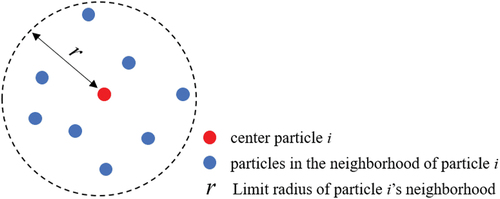
where $p_i^n$ denotes the pressure of particle $i$ in the current frame. This integral pressure feature implies the magnitude of the interaction between the centre particle and its neighbour particles in the current frame (the $n$th frame). In the MPS method, the actual pressure of the centre particle of the next frame (the $(n+1)$st frame) is a linear combination of the integral pressure feature of neighbour particles (also of the next frame), and the temporary particle number density and divergence of velocity. 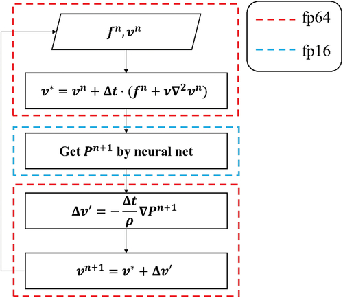For the pressure regression problem, we expect the neural network to learn a more abstract way of combination such that, given the integral feature of the $n$th frame, it can predict the pressure of the $(n+1)$st frame. The velocity update scheme is shown in Figure 3.

Figure 3. The velocity update scheme in the proposed NN-MPS method.

3.2. The training process

The basic structure of the neural network is shown in Figure 4. The depth of the hidden layers is set to three. We have found that, although deeper neural networks can reach smaller losses, they perform worse than the one of three hidden layers. The neural network is fully connected, consists of three rectified linear unit layers [21] (ReLU) and a linear activation layer. The forward propagation of the proposed neural network can be summarized as

Figure 4. A description of the neural network. For each neuron in the hidden layer, the nonlinear activation function is the ReLU. Each of the first two hidden layers has eight neurons, and the last hidden layer has four neurons.

(2) ${\hat{p}}^{n+1}=W^{(4)}\cdot f(W^{(3)}\cdot f(W^{(2)}\cdot f(W^{(1)}\cdot \theta +b^{(1)})+b^{(2)})+b^{(3)})+b^{(4)},$(2)

$f(x)=\mathrm{m}\mathrm{a}\mathrm{x}(0,x),$

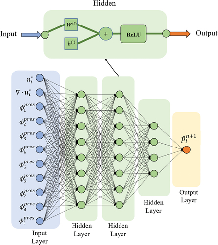
where, given the feature vector $\theta$, ${\hat{p}}^{n+1}$ is the pressure of the next frame generated by the neural network, $f$ is the nonlinear activation function ReLU, $W^{(l)}$ and $b^{(l)}$ are parameters of the $l$th layer, $l=\left\{1,2,3,4\right\}$.

The integral pressure feature of each neighbour particle is numbered according to the distance between the centre particle and it. For example, in Figure 4, ${\varphi }_1^{\mathrm{p}\mathrm{r}\mathrm{e}\mathrm{s}}$ is the integral pressure feature of the nearest particle. This numbering method can help the neural network to learn the underlying invariance of the system. The radius of neighbour is set to $1.1\times l_0$. $l_0$ is the initial distance of each particle. The reason of choosing it is that particles beyond it barely contribute to the system, see Figure 5. Then, based on this radius, we set the number of input integral pressure features to eight. If there are less than eight neighbour particles in the radius, vacant positions are filled by 0.

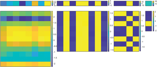
Figure 5. A Visualization of $W^l$ and $b^l$, $l=\left\{1,2,3\right\}$, in (2) after training. The vectors at the top are $b$ and the matrices at the bottom are $W$. From left to right: $1^{st}$ layer, $2^{nd}$ layer, $3^{rd}$ layer, $4^{th}$ layer.

For the learning of the pressure regressor, we measure the loss with mean squared L2-norm, i.e.

$MSE=\frac{1}{m}\sum _i^m{\left({\hat{p}}_i-p_i\right)}^2,$

where $m$ is the number of training sets, ${\hat{p}}_i$ is the outcome of the neural network. Here, we use the result of the CG method as the ground-truth label to train our neural network. The training was done in the four simple scenes shown in Table 1 and Figure 6 with a total number of a billion training samples. Namely, we apply the back propagation [22] to update the parameters in the neural network and use Adam [23], a mini-batch stochastic optimization algorithm, to optimize the loss function. We also use the dropout [24] method to avoid overfitting. The values of $W^l$ and $b^l$, $l=\left\{1,2,3,4\right\}$, in (2) after training are shown in Figure 5. It can be seen that $\mathrm{\nabla }\cdot \mathit{u}$ is negatively correlated to the results while ${\varphi }_j$ is positively correlated to the results, and the correlation decreases as the distance increases. The training process totally takes about 3–4 hours on our platform.

Figure 6. A visualization of the training set. From left to right: scene 1, scene 2, scene 3, scene 4.

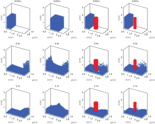
Table 1. Parameters of different scenes in the training set. The time step is set to 0.003 s and the simulation time of all scenes is 1.5 s (500 steps). The initial distance is set to 0.075. The size implies the number of particles, where $r$ is the radius, $h$ is the height, $l$ is the length and $w$ is the width.

Scene	Box size	Column size	Obstacle size	Obstacle position
1	$32\times 16\times 20$	$8\times 16\times 20$	$-$	$-$
2	$32\times 16\times 20$	$16\times 16\times 20$	$-$	$-$
3	$32\times 16\times 20$	$8\times 16\times 20$	$r=3,h=20$	$(1.4250,0.8250)$
4	$32\times 16\times 20$	$8\times 16\times 20$	$r=w=3,h=20$	$(1.4250,0.8250)$

Visualization of $W^l$ and $b^l$, $l=\left\{1,2,3\right\}$, in (2) after training. The vectors at the top are $b$ and the matrices at the bottom are $W$. From left to right: $1^{st}$ layer, $2^{nd}$ layer, $3^{rd}$ layer, $4^{th}$ layer.

4. Numerical results

4.1. Validation on workstation

The dam collapse is a benchmark problem in the simulation of free-surface flow. To illustrate the performance of the NN-MPS, we implement both the original MPS and the NN-MPS on the dam collapse problem and compare their results to those of an experiment. The parameters of this test are listed in Table 2. Figure 7 shows that particles of two methods move in a similar pattern. Pressure in NN-MPS distributes more smoothly, resulting in a less drastic velocity oscillation.

Figure 7. A visualization of the dam collapse problem. Upper: NN-MPS. Lower: Original MPS. From left to right: $0.3s,0.6s,0.9s,1.2s,1.5s$.

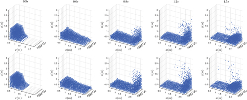
Table 2. The parameters setting for the dam collapse problem.

Parameters	Value
Initial distance for particles $l_0$	$0.075m$
Gravitational acceleration $g$	$9.81$$m^2/s$
Water kinematic viscosity $\nu$	$1\times {10}^{-6}$$m^2/s$
Coefficient of collision $e$	0.2
Time interval of each frame $\mathrm{\Delta }t$	0.003s
Tank size	$32l_0\times 16l_0\times 20l_0$
Column size	$8l_0\times 16l_0\times 18l_0$

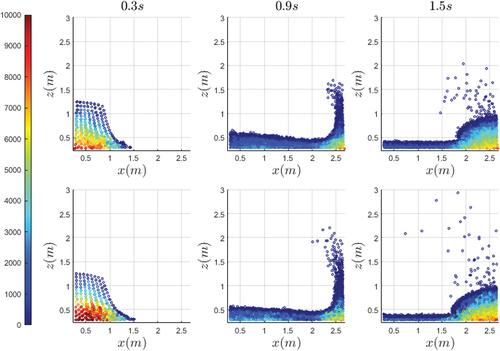
The pressure distributions at 0.3 s, 0.9 s and 1.5 s are shown in Figure 8. The pressure distributions of the NN-MPS method become more uniform compared to those of the original MPS method. From inside to the surface, particle pressure in both methods decreases due to the decreasing particle number density. However, in the original MPS method, the pressure boundary is not obvious, while that in NN-MPS is more obvious.

Figure 8. A comparison of pressure distribution at $0.3s$, $0.9s$, and $1.5s$ (from left to right). Top row: NN-MPS; Bottom row: Original MPS.

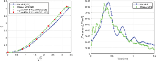
The comparison of the front position and pressure at the left-bottom corner is shown in Figure 9. In MPS and NN-MPS, the aspect ratio is 2.25, and in the experiment of J.C.Martin and W.J.Moyce [18], the aspect ratio is 1.125 and 2.25. At the beginning stage, the particles in NN-MPS move more slowly (closer to the experimental results) than MPS. After a while, the MPS results become closer to those of the experimental data. For the pressure, NN-MPS suffers a slightly larger oscillation period and amplitude than MPS. Overall, the changing patterns of pressure in both methods are similar.

Figure 9. A comparison of the position of fluid front and pressure at bottom of the left wall.

We also applied NN-MPS to two dam collapse with obstacle problems. In these problems, particles out of the right-side boundary ($x=36l_0$) will not be calculated anymore. Physics parameters (except those of the obstacles) are set to be the same as the dam collapse problem. The radius of the cylinder obstacle is $4l_0$. As shown in Figures 11–12, visually there are few differences between the results of NN-MPS and MPS. The pressure and $z$ component of the pressure gradient are compared in Figure 10. In both cases, the NN-MPS results show a slightly larger oscillation in the early stage, but gradually approach the MPS results.

Figure 10. The pressure and the pressure gradient of flow field. Left: With one-cylinder obstacle. Right: With a two-cylinder obstacle. Upper: Pressure at bottom of the left wall. Lower: $z$ component of pressure gradient at bottom of the left wall.

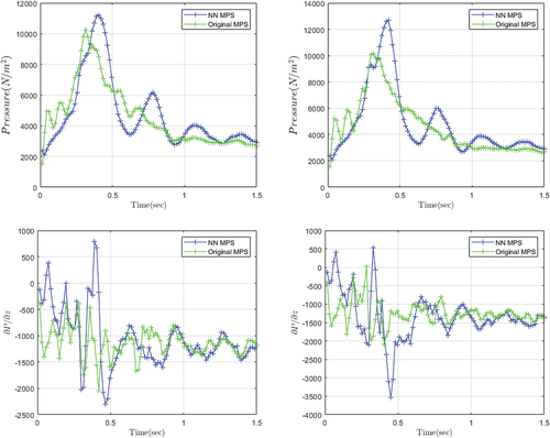
Figure 11. A comparison of two algorithms on the problem with a one-cylinder obstacle. Top row: NN-MPS. Bottom row: MPS.

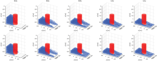
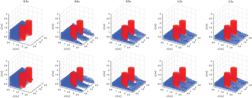
Figure 12. A comparison of two algorithms on the problem with a two-cylinder obstacle. Top row: NN-MPS. Bottom row: MPS.

4.2. Efficiency comparison

The profile of devices used for this test is as follows: Intel Core i7-6820HK @ 2.70 GHz, 16.0GB memory, Nvidia GTX 1070. The algorithms are mainly implemented in Python. The regression model is constructed using the deep-learning module Tensorflow [25] and is trained on GPU. The calculations are conducted on both CPU and GPU. The GPU implementation of NN-MPS uses CUDA. The parameters used for these tests are shown in Table 3.

Table 3. The parameters setting for the dam collapse problem.

Case	Description	Box size	Total particle numbers	Pressure caculation using time
				MPS	NN-MPS(CPU)	NN-MPS(GPU)
1	Column collapse(1)	$32l_0\times 16l_0\times 16l_0$	13056	1.45s	0.42s	0.04s
2	Column collapse(2)	$64l_0\times 32l_0\times 32l_0$	54528	16.93s	3.55s	0.05s
3	Column collapse(3)	$96l_0\times 48l_0\times 48l_0$	136962	86.97s	9.92s	0.11s
4	One-cylinder obstacle	$40l_0\times 16l_0\times 16l_0$	15316	1.45s	0.42s	0.04s
5	Two-cylinder obstacle	$40l_0\times 32l_0\times 16l_0$	13056	1.45s	0.42s	0.04s

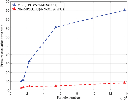
Results are shown in Figure 13. As the scale of the problem increases, the pressure calculation time in MPS can increase in a relatively large rate. In contrast, the increasing rate of the pressure prediction time in NN-MPS is almost linear to the total particle number. Moreover, the pressure calculation in NN-MPS is independent for each particle. Thus, the algorithm can be parallelized efficiently on GPU. Since GPU has much more processing units and threads than CPU, it can outperform CPU on computing efficiency by far. The efficiency of the GPU implementation of NN-MPS is nearly 50 times of that of the CPU implementation.

Figure 13. The ratio of pressure calculation time.

5. Edge computing

Our final goal is to achieve the real-time simulation. One alternative way is to use hardwares to speedup the computation. In the previous section, we have used the GPU to accelerate the computation. While in this part, we choose an edge computing device, which is cheaper and needs lower electrical power to achieve a more efficient computation.

5.1. Introduction to edge computing and DaVinci architecture

Edge computing is a distributed computing framework that computes data at its source and requires a quicker response and a lower power consumption. Atlas 200DK Developer Kit (or, shortly, Atlas 200DK) is a high-performance AI application development board for edge computing scenarios.

In this part, Atlas 200DK is taken as an example to demonstrate how to apply NN-MPS to edge computing and how well it works. Ascend 310 is the main computing chip of Atlas 200DK which consists of two AI cores (Da Vinci architecture) and eight AI CPUs. The DaVinci architecture has three kinds of basic computing units, i.e. cube, vector and scalar units, which provide high-speed matrix, vector, and scalar computing. These AI cores are extremely efficient for neural network thus is possible to speedup up the computation of NN-MPS.

To run NN-MPS more effectively on Ascend 310, two important adjustments must be made: using AI Core to accelerate the neural network process and working with a high-efficiency parallel algorithm to make full use of all the AI CPUs.

5.2. Multi-precision and parallel strategy

One of the ways AI core accelerates computation is to reduce floating-point precision to reduce floating-point computation time. Therefore, the floating-point precision of the AI core is reduced to 16 bits. Sixteen bits floating-point consists of one sign bit, five exponential bits, and ten bits for fraction, it can be calculated with an accuracy up to four significant digits.

Lower precision will lead to a bad influence on the simulation results. However, in our numerical tests, this influence is limited as will shown in Section 5.3. Therefore, the accuracy loss of running the neural network on AI cores is acceptable. Figure 14 shows the multi-precision strategy used in this paper.

Figure 14. An illustration of the multi-precision strategy used on ascend 310.

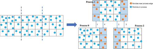
The parallelization is as follows: Firstly, as shown in the left diagram of Figure 15, the flow field is evenly divided into rectangular grids based on the search strategy, i.e. the linked-list method. Then, these grids are divided into several parts along the $x$-axis. Each part is computed by a single process. As shown in the right diagram of Figure 15, since each particle pressure depends only on particles nearby, each process only needs to store some buffer particles of its neighbour processes. For each time step, the only communication between processes is exchanging their buffer particles.

Figure 15. A description of dividing the domain into grids and distributing the grids to different processes.

5.3. Numerical results

The three testing models shown in Figure 16 are used to demonstrate the reliability and superiority of NN-MPS on the edge computing device. Details are shown in Table 4.

Figure 16. A visualization of three testing models.

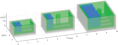
Table 4. The model sizes and speedup.

Index	Box size	Fluid particles	CPU	AI core	Speedup
1	$[30,20,14]\times 0.075$	1456	0.2932s	0.035s	8.37815
2	$[40,24,20]\times 0.075$	2048	0.2955s	0.036s	8.2077
3	$[40,48,20]\times 0.075$	10240	0.5882s	0.12052s	4.8805

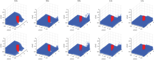
The running times in the blue box in Figure 14 are measured and displayed in Table 4. AI Cores lead to a significant improvement on the pressure-solving time thanks to their high efficiency for neural networks. The results of free-surface motion are also shown to show that the increase in efficiency does not cause a decrease in accuracy. As shown in Figure 17(a), $X$ is the motion of the fluid front, and $H$ is the height of the fluid on the left edge. Results are shown in Figures 17(b), Figures 17(c) and 17(d). It is easy to see that the results of free-surface motion have very low error. The pressure results at the left-bottom corner are also shown in Figure 18. There is an error in the results, but the error is limited. And as shown in Figures 19–21, the results of two different devices are visually the same.

Figure 17. Numerical results of the free-surface movement. (a) shows the definition of $X$ and $H$. (b), (c) and (d) respectively show the results of models with index number 1, 2 and 3.

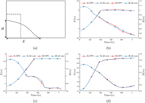
Figure 18. Pressure results at left corner. (a), (b) and (c) respectively show the results of models with index number 1, 2 and 3.

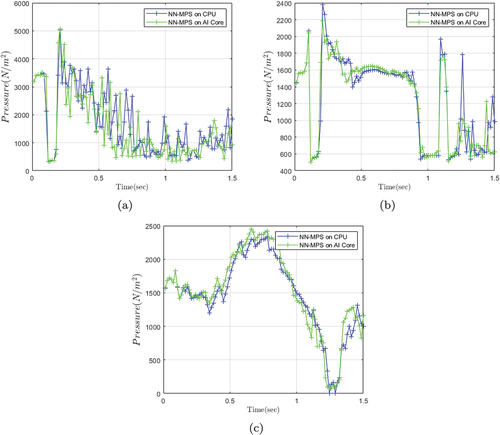
Figure 19. A comparison of two different devices on the problem with case 1. Top row: CPU. Bottom row: AI Core.

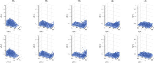
Figure 20. A comparison of two different devices on the problem with case 2. Top row: CPU. Bottom row: AI Core.

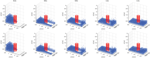
Figure 21. A comparison of two different devices on the problem with case 3. Top row: CPU. Bottom row: AI Core.

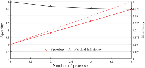
Results of the parallel speedup and efficiency are shown in Figure 22. The efficiency is as high as 87.5% with four computing processes, which shows the superiority of NN-MPS in parallel computing.

Figure 22. The parallel efficiency and speedup.

6. Summary and discussion

A novel machine learning method to accelerate the pressure calculation of the MPS method is proposed in this work. According to our tests, the neural network regressor we built can successfully learn the underlying pressure variation pattern and maintain the robustness. Since the projection through a neural network does not require iterations, it can significantly improve the simulation efficiency. Moreover, our work can attain a similar effect with a relatively small neural network. This characteristic further helps saving computational resources. The proposed NN-MPS shows clear computational cost improvement for free-surface flows and does not sacrifice accuracy for the pressure computation.

Like many other machine learning techniques and data-driven approaches, a weakness of the proposed method is that it cannot be generalized to other cases that are too different from the training data (e.g. flows with different physics parameters such as particle mass, density, viscosity, etc.). Another problem is that, in every frame, the continuity equation cannot be entirely satisfied; the average particle number density sometimes deviates from the initial constant $N^0$. However, this error will not accumulate, and the NN-MPS can maintain the convergence even after hundreds of time steps. Since the neural network is used to solve a pressure Poisson equation with specific spatial and temporal resolutions, different values of these two parameters can lead to totally different solutions. As a result, the NN-MPS cannot run with training sets of different spatial and temporal resolutions. However, as a particle method, we can run many different cases with the same resolution and different geometries, which extends the application scenario of this method.

The introduction of the neural network provides MPS an opportunity for the usage of advanced computing deep learning hardwares, and the feature of not relying on all particles in the computing domain makes it easier to be parallelized. By running on special AI hardware, the computation time of the pressure Poisson equation is further reduced. The results also show the possibility to reach a high speed with a good parallel strategy. Discussions about running NN-MPS on the edge computing device shows the potential for the NN-MPS method to realize real-time simulation in the future.

Future works of this research include the implementation of geographical phenomena simulations and realistic graphics rendering to demonstrate its functionality on practical problems with limited computational resources. The time interval in the simulation requires further study, which has a significant influence on the simulation speed. In this study, we only adapt the constant time interval criterion from the MPS method. The pressure oscillation is also an important aspect for further improvements. We will also consider some ways (e.g. methods in [26–28]) to reduce the pressure oscillation.

Disclosure statement

No potential conflict of interest was reported by the author(s).

Additional information

Funding

The work was supported by the National Natural Science Foundation of China [11972384]. The National Key R&D program for International Collaboration [2020YFA0712502] and Guangdong Science and Technology Fund [2021B1515310001] also supported this work.

References

- ] S. Koshizuka, Y. Oka, Moving-particlesemi-implicit method for fragmentation of incompressible fluid, Nucl. Sci. Eng. 123, 3 (1996), pp. 421–434. doi:10.13182/NSE96-A24205
- J.J. Monaghan, Smoothed particle hydrodynamics, Annu. Rev. Astron. Astrophys. 30 (1) (1992), pp. 543–574. doi:10.1146/annurev.aa.30.090192.002551.
- A.M. Gambaruto, Computational haemodynamics of small vessels using the moving particle semi-implicit (mps) method, J. Comput. Phys. 302 (2015), pp. 68–96. doi:10.1016/j.jcp.2015.08.039.
- K. Murotani, S. Koshizuka, T. Tamai, K. Shibata, N. Mitsume, S. Yoshimura, S. Tanaka, K. Hasegawa, E. Nagai, and T. Fujisawa, Development of hierarchical domain decomposition explicit mps method and application to large-scale tsunami analysis with floating objects, Adv. Model. Simul. Eng. Sci. 1 (1) (2014), pp. 16–35. doi:10.15748/jasse.1.16.
- T. Okabe, H. Matsutani, T. Honda, and S. Yashiro, Numerical simulation of microscopic flow in a fiber bundle using the moving particle semi-implicit method, composites part A, Appl. Sci. Manuf. 43 (10) (2012), pp. 1765–1774. doi:10.1016/j.compositesa.2012.05.003.
- G. Duan and B. Chen, Comparison of parallel solvers for moving particle semi-implicit method, Eng. Comput. 32 (3) (2015), pp. 834–862. doi:10.1108/EC-02-2014-0029.
- S. Koshizuka, K. Shibata, M. Kondo, and T. Matsunaga, Moving Particle Semi-Implicit Method: A Meshfree Particle Method for Fluid Dynamics, Cambridge, Massachusetts: Academic Press, 2018.
- B.R. Noack and H. Eckelmann, A low-dimensional galerkin method for the three-dimensional flow around a circular cylinder, Phys. Fluids 6 (1) (1994), pp. 124–143. doi:10.1063/1.868433.
- A. Treuille, A. Lewis, and Z. Popović, Model reduction for real-time fluids, ACM Trans. Graph. 25 (3) (2006), pp. 826–834. doi:10.1145/1141911.1141962.
- R. Ando, N. Thürey, and C. Wojtan, A dimension-reduced pressure solver for liquid simulations, in Computer Graphics Forum, Vol. 34, Hoboken, New Jersey, U.S: Wiley Online Library, 2015, pp. 473–480.
- T. De Witt, C. Lessig, and E. Fiume, Fluid simulation using Laplacian eigenfunctions, ACM Trans. Graph. 31 (1) (2012), pp. 1–11. doi:10.1145/2077341.2077351.
- S. Li, G. Duan, and M. Sakai, Development of a reduced-order model for large-scale Eulerian–Lagrangian simulations, Adv. Powder Technol. 33 (8) (2022), pp. 103632. doi:10.1016/j.apt.2022.103632.
- L. Ladickỳ, S. Jeong, B. Solenthaler, M. Pollefeys, and M. Gross, Data-driven fluid simulations using regression forests, ACM Trans. Graph. 34 (6) (2015), pp. 1–9. doi:10.1145/2816795.2818129.
- Z. Li and A.B. Farimani, Graph neural network-accelerated Lagrangian fluid simulation, Comput. Graph 103 (2022), pp. 201–211. doi:10.1016/j.cag.2022.02.004.
- J. Bai, Y. Zhou, Y. Ma, H. Jeong, H. Zhan, C. Rathnayaka, E. Sauret, and Y. Gu, A general neural particle method for hydrodynamics modeling, Comput. Methods Appl. Mech. Eng. 393 (2022), pp. 114740. doi:10.1016/j.cma.2022.114740.
- C. Yang, X. Yang, and X. Xiao, Data-driven projection method in fluid simulation, Comput. Animat Virtual. Worlds 27 (3–4) (2016), pp. 415–424. doi:10.1002/cav.1695.
- J. Tompson, K. Schlachter, P. Sprechmann, and K. Perlin, Accelerating Eulerian fluid simulation with convolutional networks, in: International Conference on Machine Learning, PMLR, Sydney, Australia, 11-15 Aug. 2017, pp. 3424–3433.
- J.C. Martin, W.J. Moyce, J. Martin, W. Moyce, W.G. Penney, A. Price, and C. Thornhill, Part iv. an experimental study of the collapse of liquid columns on a rigid horizontal plane, Philos Trans. R. Soc. Lond A 244 (1952), pp. 312–324.
- L. Hernquist and N. Katz, Treesph-a unification of sph with the hierarchical tree method, Astrophys. J., Suppl. Ser. 70 (1989), pp. 419–446. doi:10.1086/191344.
- B.-H. Lee, J.-C. Park, M.-H. Kim, and S.-C. Hwang, Step-by-step improvement of mps method in simulating violent free-surface motions and impact-loads, Comput. Methods Appl. Mech. Eng. 200 (9–12) (2011), pp. 9–12. doi:10.1016/j.cma.2010.12.001.
- V. Nair and G.E. Hinton, Rectified linear units improve restricted Boltzmann machines, ICML'10: Proceedings of the 27th International Conference on International Conference on Machine Learning. icml10 (2010), pp. 807–814.
- D.E. Rumelhart, G.E. Hinton, and R.J. WilliamsLearning representations by back-propagating errors, nature32360881986533–536.10.1038/323533a0.
- D.P. Kingma and J. Ba. Adam: A method for stochastic optimization. In International Conference on Learning Representations, San Diego, USA, 7-9. May. 2015, ICLR (Poster) 2015 Ithaca, NY: arXiv.org, 2015. https://arxiv.org/pdf/1412.6980.pdf
- N. Srivastava, G. Hinton, A. Krizhevsky, I. Sutskever, and R. Salakhutdinov, Dropout: A simple way to prevent neural networks from overfitting, J. Mach. Learn. Res. 15 (2014), pp. 1929–1958.
- M. Abadi, P. Barham, J. Chen, Z. Chen, A. Davis, J. Dean, M. Devin, S. Ghemawat, G. Irving, M. Isard, Manjunath, Kudlur, Josh, Levenberg, Rajat, Monga, Sherry, Moore, Derek, G., Murray, Benoit, Steiner, Paul, Tucker, Vijay, Vasudevan, Pete, Warden, Martin Wicke, Yuan Yu, Xiaoqiang Zheng. TensorFlow: A system for large-scale machine learning. In 12th USENIX Symposium on Operating Systems Design and Implementation (OSDI '16), NOVEMBER 2–4, 2016, SAVANNAH, GA, USA, Vol. 16. 2016, pp. 265–283.
- L. Wang, A. Khayyer, H. Gotoh, Q. Jiang, and C. Zhang, Enhancement of pressure calculation in projection-based particle methods by incorporation of background mesh scheme, Appl. Ocean Res. 86 (2019), pp. 320–339. doi:10.1016/j.apor.2019.01.017.
- G. Duan, S. Koshizuka, A. Yamaji, B. Chen, X. Li, and T. Tamai, An accurate and stable multiphase moving particle semi-implicit method based on a corrective matrix for all particle interaction models, Int. J. Numer Methods Eng. 115 (10) (2018), pp. 1287–1314. doi:10.1002/nme.5844.
- G. Duan, T. Matsunaga, S. Koshizuka, A. Yamaguchi, and M. Sakai, New insights into error accumulation due to biased particle distribution in semi-implicit particle methods, Comput. Methods Appl. Mech. Eng. 388 (2022), pp. 114219. doi:10.1016/j.cma.2021.114219.