Quadratic upwind differencing scheme in the finite volume method for solving the convection-diffusion equation

ABSTRACT

Due to the high importance of the convection-diffusion equation, we aim to develop a quadratic upwind differencing scheme in the finite volume approach for solving this equation. Our newly developed numerical approach is conditionally stable. The strategy employs a quadratic upwind differencing scheme in the finite volume technique for spatial approximation with third-order accuracy. The temporal integration is approximated using the explicit theta method of first-order accuracy. Some numerical examples are given to support our theoretical procedures. The findings are plotted using MATLAB R2016a mathematical software.

KEYWORDS:

• Convection-diffusion equation
• quadratic upwind differencing scheme
• finite volume method

1. Introduction

Many key phenomena in chemical diffusion, fluid flow, heat transfer, ocean circulation, signal processing, solid mechanics, wave propagation, and other fields are well governed by partial differential equations [1]. The convection-diffusion equation is a mathematical model that depicts a substance’s concentration in fluid dynamics and heat transfer [2]. The equation is a combination of convection and diffusion terms and has several applications in engineering and science fields [3,4]. Convection and diffusion equations are the two physical processes that appear in several applications in the transfer of particles and other quantities inside a physical system [5,6]. Starting and boundary value problems like unsteady state second-order convection-diffusion equations are highly important in mathematics and engineering. Based on the convection or diffusion rate, the convection-diffusion equation can be convection or diffusion dominated. The diffusion coefficient can be calculated with the help of Fick’s laws of diffusion [7]. The second law of Fick is similar to the diffusion equation [7]. For fluid transport, Buckman [8] stated a derivation of the convection-diffusion equation.

Finding accurate and effective techniques for solving partial differential equations has become a focus of ongoing study. Several techniques to calculate an exact value of some linear and nonlinear equations have recently been developed and now received considerable attention of researchers. Nowadays, different scholars focus on techniques for finding analytic results rather than approximate values. With the help of the Lie symmetry approach, M. Usman et al. [9] solved the 1D wave propagation in phononic materials based on the simplified micromorphic model. After constructing optimal system of Lie subalgebras, they converted a system into ordinary differential equations. Based on Laplace transform technique and using the variational iteration method, the authors of [10] computed the analytic results for nonlinear oscillators. Hussain, Kara and Zaman [11] solved the Vakhnenko – Parkes equation using the Lie symmetry transformation approach. They construct the discrete symmetries of this equation with the help of a modified Hydon’s approach. A. Hussain et al. [12] focused on the analysis of the Peyrard – Bishop DNA dynamic model equation. Jacobi elliptic function expansion and Lie symmetry approaches were used to compute an exact value of the model. In Ref [13], the thermophoretic equation was solved analytically with the help of wrinkle propagation in substrate-supported Graphene sheets. Using Lie symmetry method, the authors of [14] discussed the Riabouchinsky Proudman Johnson equation and achieved first-time explicit analytical results. For additional reading on other direct methods to compute the analytic results of differential equations, an interesting reader is referred to in [15–17]. From these discussions, we understood that numerous techniques for finding an accurate solution are available. Fluid dynamics is a scientific field of huge significance in applied mathematics, where crucial equations are typically stated using partial differential equations. Such an equation has an exact result only possible for some cases [18]. Most of the time, finding an exact solution to a partial differential equation is challenging. As a result, considerable attention must be given to the effective numerical schemes that converge to the exact result.

The primary aim of the current study is to develop a quadratic upwind interpolation for convective kinematics (QUICK) approach in the finite volume method (FVM) for solving convection-diffusion problem. The main advantage of numerical schemes in the FVM lies in their accuracy for the computation of fluid flow dynamics [19]. A significant aim of the schemes is to reduce the differential equation into a system of algebraic equations [20]. The FVM can be used for different engineering issues that are represented by the differential equations. The definite integration of the given problem over a control volume is a key step of the FVM. Several engineering and science issues have recently been solved in different schemes of the FVM. OpenFOAM (Open-Source Field Operation and Manipulation) for computational hydrodynamics using the FVM was investigated by the authors in [21]. Muhammad and Ullah [22] studied the simulation of flow on the hydroelectric power dam spillway through OpenFOAM with the help of the FVM. Using the large eddy simulation mode, authors of [23] discussed the simulation of turbulence flow in OpenFOAM. The simulation was based on the finite volume method. In a higher methane-cut reservoir, authors in [24] studied the energy recovery mechanism of air injection and approximated their results using the FVM. The finite volume technique was applied for approximating combustion dynamics via OpenFOAM in [25]. An article in [26] focused on the analysis of fluid flow through OpenFOAM using the FVM. For the approximate results of the convection-diffusion equation (CDE), various schemes in the FVM have been established. Hussain, Zheng, and Fekadie in [27], studied the CDE using a modified upwind scheme. With the second-order accuracy, the technique was unconditionally stable. The Crank-Nicolson formulation was used to approximate in the temporal direction. We have studied this problem using a quadratic upwind differencing scheme. Unsteady 1D convection-diffusion equations were solved using a high-order exponential technique by the authors of [28]. The developed technique was unconditionally stable and has fourth-order accuracy. In [29], an upwind technique was used to discretize a singularly perturbed CDE. The authors in [30], studied a 1D unsteady state CDE using fully implicit hybrid and central differencing schemes in the finite volume approach. Edwan et al. [31] solved the fractional-order CDE in Riemann-Liouville fractional operator with the help of finite volume technique. The scheme was conditionally stable, with first and second order accuracy in time and in space, respectively. Using finite volume approach, Saddeh [32] obtained the results of fractional order CDE. Patel and Pandya [33] used the FVM to approximate 1D unsteady state and 2D steady state heat transfer equations with starting and boundary values. Authors of [34] approximated convection and convection-diffusion equations using an Eulerian-Lagrangian Runge-Kutta FVM. In [35], the convection-diffusion equations with Dirichlet and Neumann boundary values were solved using the FVM. A conservative semi-Lagrangian finite volume technique was used to compute the convection-diffusion problem on unstructured grids [36]. For solving convection-diffusion-reaction equation, Mingtian [37] applied the finite volume technique. For additional reading on other numerical schemes for solving CDE an interesting reader is referred to [38–43].

Leonard developed the QUICK scheme in the finite volume approach for the first time in 1979 [44]. This scheme is now gaining more popularity due to its high range of application in practical computational fluid dynamics [45]. A quadratic upwind differencing scheme (or QUICK scheme) is a powerful approximate scheme used for finding solution of convection-diffusion equation. A comparison between the solutions obtained by the QUICK approach in the FVM and the solutions existing in the literature shows that our solutions are more general, and novel, and have never been reported earlier. This paper aims to present QUICK scheme to the control volume technique for solving a single-domain convection-diffusion equation. A single-domain problem is used, which does not require interface tracking and allows the use of a fixed grid in order to solve the governing equations [46,47]. Numerical schemes in the finite volume approach are adaptable to the bidomain problems [48–51]. A major drawback of the bidomain scheme is its complexity of implementation. Because of the computational cost of the bidomain scheme, here we discuss the convection-diffusion problem in a single domain. In spatial discretization, our newly proposed technique is conditionally stable and has third-order accuracy. In this work, we use the explicit theta method $\left(\theta =0\right)$ with first order accuracy in time for temporal approximation. In our methodology, the approximate findings are presented in the absence of the thermophoresis effect. The existence of our solution in the presence of thermophoresis effect is not checked, which is a limitation of this study. This paper will provide an extensive understanding of a QUICK scheme in the FVM for computational fluid dynamics simulation and analysis. The study’s findings will serve as a basis for future research in this field by other scholars. It will contribute to the existing literature on numerical approaches for approximating convection-diffusion equations. The findings of this study may help students and academics to design higher-order schemes in the future for approximating mathematical problems. There are so many studies related to this mathematical problem that the proposed approach can be seen as an essential addition to attracting interest among fluid dynamics researchers. Our objective in the present study is to use the quadratic upwind differencing scheme to find the approximate solution for the convection-diffusion equation that will help the reader in this subject area. The paper’s structure is as follows: The discretization and formulation of the problem are covered in Section 2. Assessment of the quick scheme is found in Section 3. To show the effectiveness of our scheme, some examples and discussions are presented in Section 4. At the end, in Section 5, a conclusion is written.

2. Discretization and formulation of the problem

Diffusion always exists alongside with convection. Thus, now we proposed the QUICK scheme in the FVM to approximate convection-diffusion equation. With no source term, a linear unsteady state convection-diffusion of a property $f$ is governed by [27] as follow:

(1) $\left\{\begin{array}{c}\frac{\mathrm{\partial }f}{\mathrm{\partial }t}+u\frac{\mathrm{\partial }f}{\mathrm{\partial }x}=h\frac{{\mathrm{\partial }}^{2}f}{\mathrm{\partial }{x}^2},0\le x\le L\mathrm{a}\mathrm{n}\mathrm{d}0\le t\le T,\\ f(x,0)=l(x),\\ f\left(0,t\right)=l_1(t),f\left(\mathrm{L},\mathrm{t}\right)=l_2(t).\end{array}\right.$(1)

where $u>0$ is convective velocity, $h\ge 0$ is diffusion coefficient, $u\frac{\mathrm{\partial }f}{\mathrm{\partial }x}$ is a convective term, and $h\frac{{\mathrm{\partial }}^{2}f}{\mathrm{\partial }{x}^2}$ is a diffusive term. The discretization of the convection and diffusion terms is the computation of the value of transported property $f$ at control volume faces and its convective flux across these boundaries. A definite integration of the CDE over a control volume (CV) gives a set of discretized equations. The local Peclet number $\left(P_{\mathrm{\Delta }}=\frac{u\mathrm{\Delta }x}{h}\right)$ is used to measure the effect of convection on the transport of physical quantities. Discretization and formulation of the same problem were investigated with the help of modified upwind scheme in the FVM by the authors of [27,52]. In this paper, we aim to solve the convection-diffusion problem with the help of a quadratic upwind differencing approach in the FVM. The quadratic upwind differencing approach of Leonard (1979 [44]) uses a three-point upstream-weighted quadratic interpolation for cell face values. The face value of $f$ is produced from a quadratic function via two bracketing nodes (on each side of the face) and a node on the upstream side (see Figure 1). For the discretization, we used the domains $\mathrm{\Pi }=\left[0,\mathrm{L}\right]$ and $\mathrm{\Delta }x=\frac{\mathrm{L}}{n},\mathrm{\Delta }t=\frac{\mathrm{T}}{m},0\le i\le n$ and $0\le j\le m$.

Figure 1. Quadratic profiles of the QUICK scheme.

Over a control volume $\left[x_{i-\frac{\mathrm{\Delta }x}{2}},x_{i+\frac{\mathrm{\Delta }x}{2}}\right]\left[t_j,t_{j+1}\right]$ around the nodal point $i$, definite integration of the governing equation (1) gives:

${\int }_{i-\frac{\mathrm{\Delta }x}{2}}^{i+\frac{\mathrm{\Delta }x}{2}}{\int }_j^{j+1}\frac{\mathrm{\partial }f}{\mathrm{\partial }t}dtdx+u{\int }_j^{j+1}{\int }_{i-\frac{\mathrm{\Delta }x}{2}}^{i+\frac{\mathrm{\Delta }x}{2}}\frac{\mathrm{\partial }f}{\mathrm{\partial }x}dxdt=h{\int }_j^{j+1}{\int }_{i-\frac{\mathrm{\Delta }x}{2}}^{i+\frac{\mathrm{\Delta }x}{2}}\frac{{\mathrm{\partial }}^{2}f}{\mathrm{\partial }{x}^2}dxdt,$

(2) ${\int }_{i-\frac{\mathrm{\Delta }x}{2}}^{i+\frac{\mathrm{\Delta }x}{2}}\left(f_{i,j+1}-f_{i,j}\right)dx+u{\int }_j^{j+1}\left(f_{i+\frac{\mathrm{\Delta }x}{2},j}-f_{i-\frac{\mathrm{\Delta }x}{2},j}\right)dt=h{\int }_j^{j+1}\left[{\left(\frac{\mathrm{\partial }f}{\mathrm{\partial }x}\right)}_{i+\frac{\mathrm{\Delta }x}{2},j}-{\left(\frac{\mathrm{\partial }f}{\mathrm{\partial }x}\right)}_{i-\frac{\mathrm{\Delta }x}{2},j}\right]dt.$(2)

For numerical integration, approximate the first term of eq. (2) using Simpson’s $1/3$ rule:

$\frac{\mathrm{\Delta }x}{3}\left(f_{i+\frac{\mathrm{\Delta }x}{2},j+1}+4f_{i,j+1}+f_{i-\frac{\mathrm{\Delta }x}{2},j+1}\right)-\frac{\mathrm{\Delta }x}{3}\left(f_{i+\frac{\mathrm{\Delta }x}{2},j}+4f_{i,j}+f_{i-\frac{\mathrm{\Delta }x}{2},j}\right)+u{\int }_j^{j+1}\left(f_{i+\frac{\mathrm{\Delta }x}{2},j}-f_{i-\frac{\mathrm{\Delta }x}{2},j}\right)dt$

(3) $=h{\int }_j^{j+1}\left[{\left(\frac{\mathrm{\partial }f}{\mathrm{\partial }x}\right)}_{i+\frac{\mathrm{\Delta }x}{2},j}-{\left(\frac{\mathrm{\partial }f}{\mathrm{\partial }x}\right)}_{i-\frac{\mathrm{\Delta }x}{2},j}\right]dt.$(3)

The QUICK differencing scheme computes $f_{i+\frac{\mathrm{\Delta }x}{2},j}$ at the east face of the ${\mathrm{i}}^{th}$ CV as

(4) $f_{i+\frac{\mathrm{\Delta }x}{2},j}=-\frac{1}{8}{f}_{i-1,j}+\frac{6}{8}{f}_{i,j}+\frac{3}{8}{f}_{i+1,j}+\mathcal{O}\left(\mathrm{\Delta }{x}^3\right).$(4)

and

(5) ${\left(\frac{\mathrm{\partial }f}{\mathrm{\partial }x}\right)}_{i+\frac{\mathrm{\Delta }x}{2},j}=\frac{-f_{i,j}+f_{i+1,j}}{\mathrm{\Delta }x}+\mathcal{O}\left(\mathrm{\Delta }{x}^3\right).$(5)

The QUICK differencing scheme computes $f_{i-\frac{\mathrm{\Delta }x}{2},j}$ at the west face of the ${\mathrm{i}}^{th}$ CV as

(6) $f_{i-\frac{\mathrm{\Delta }x}{2},j}=-\frac{1}{8}{f}_{i-2,j}+\frac{6}{8}{f}_{i-1,j}+\frac{3}{8}{f}_{i,j}+\mathcal{O}\left(\mathrm{\Delta }{x}^3\right).$(6)

and

(7) ${\left(\frac{\mathrm{\partial }f}{\mathrm{\partial }x}\right)}_{i-\frac{\mathrm{\Delta }x}{2},j}=\frac{-f_{i-1,j}+f_{i,j}}{\mathrm{\Delta }x}+\mathcal{O}\left(\mathrm{\Delta }{x}^3\right).$(7)

The appendix section contains a detailed explanation of equations (4)-(7). Now substitute the approximations given in Eqs. (4), (5), (6) and (7) into eq. (3) and after some rearrangements, we arrived at:

$-\frac{\mathrm{\Delta }x}{24}{f}_{i-2,j+1}+\frac{5\mathrm{\Delta }x}{24}{f}_{i-1,j+1}+\frac{41\mathrm{\Delta }x}{24}{f}_{i,j+1}+\frac{\mathrm{\Delta }x}{8}{f}_{i+1,j+1}$

(8) $+\frac{u}{8}{\int }_j^{j+1}{f}_{i-2,j}dt+\left[-\frac{7u}{8}-\frac{h}{\mathrm{\Delta }x}\right]{\int }_j^{j+1}{f}_{i-1,j}dt+\left[\frac{3u}{8}+\frac{2h}{\mathrm{\Delta }x}\right]{\int }_j^{j+1}{f}_{i,j}dt$(8)

$+\left[\frac{3u}{8}-\frac{h}{\mathrm{\Delta }x}\right]{\int }_j^{j+1}{f}_{i+1,j}dt=-\frac{\mathrm{\Delta }x}{24}{f}_{i-2,j}+\frac{5\mathrm{\Delta }x}{24}{f}_{i-1,j}+\frac{41\mathrm{\Delta }x}{24}{f}_{i,j}+\frac{\mathrm{\Delta }x}{8}{f}_{i+1,j}.$

Theta method is applied for temporal integration:

(9) ${\int }_j^{j+1}{f}_{i}dt=\left(\theta f_{i,j+1}+(1-\theta )f_{i,j}\right)\mathrm{\Delta }t,$(9)

where $\theta \in \left[0,1\right]$.

$-\frac{\mathrm{\Delta }x}{24}{f}_{i-2,j+1}+\frac{5\mathrm{\Delta }x}{24}{f}_{i-1,j+1}+\frac{41\mathrm{\Delta }x}{24}{f}_{i,j+1}+\frac{\mathrm{\Delta }x}{8}{f}_{i+1,j+1}$

(10) $+\theta \mathrm{\Delta }t\left[\frac{u}{8}{f}_{i-2,j+1}+\left(-\frac{7u}{8}-\frac{h}{\mathrm{\Delta }x}\right)f_{i-1,j+1}+\left(\frac{3u}{8}+\frac{2h}{\mathrm{\Delta }x}\right)f_{i,j+1}+\left(\frac{3u}{8}-\frac{h}{\mathrm{\Delta }x}\right)f_{i+1,j+1}\right]$(10)

$+(1-\theta )\mathrm{\Delta }t\left[\frac{u}{8}{f}_{i-2,j}+\left(-\frac{7u}{8}-\frac{h}{\mathrm{\Delta }x}\right)f_{i-1,j}+\left(\frac{3u}{8}+\frac{2h}{\mathrm{\Delta }x}\right)f_{i,j}+\left(\frac{3u}{8}-\frac{h}{\mathrm{\Delta }x}\right)f_{i+1,j}\right]$

$=-\frac{\mathrm{\Delta }x}{24}{f}_{i-2,j}+\frac{5\mathrm{\Delta }x}{24}{f}_{i-1,j}+\frac{41\mathrm{\Delta }x}{24}{f}_{i,j}+\frac{\mathrm{\Delta }x}{8}{f}_{i+1,j}.$

For explicit scheme $\left(\theta =0\right)$ with first order accuracy in time and divide by $\mathrm{\Delta }x$, we arrived to the following discretized form:

$-\frac{1}{24}{f}_{i-2,j+1}+\frac{5}{24}{f}_{i-1,j+1}+\frac{41}{24}{f}_{i,j+1}+\frac{1}{8}{f}_{i+1,j+1}=\left(-\frac{1}{24}-\frac{u\mathrm{\Delta }t}{8\mathrm{\Delta }x}\right)f_{i-2,j}$

(11) $+\left(\frac{5}{24}+\frac{7u\mathrm{\Delta }t}{8\mathrm{\Delta }x}+\frac{h\mathrm{\Delta }t}{\mathrm{\Delta }{x}^2}\right)f_{i-1,j}+\left(\frac{41}{24}-\frac{3u\mathrm{\Delta }t}{8\mathrm{\Delta }x}-\frac{2h\mathrm{\Delta }t}{\mathrm{\Delta }{x}^2}\right)f_{i,j}+\left(\frac{1}{8}-\frac{3u\mathrm{\Delta }t}{8\mathrm{\Delta }x}+\frac{h\mathrm{\Delta }t}{\mathrm{\Delta }{x}^2}\right)f_{i+1,j}.$(11)

Similarly, for the quadratic downwind approach $\left(u<0\right)$, we have defined the upstream nodes and in the case of the quadratic downwind approach.

(12) $f_{i+\frac{\mathrm{\Delta }x}{2},j}=-\frac{1}{8}{f}_{i+2,j}+\frac{3}{8}{f}_{i,j}+\frac{6}{8}{f}_{i+1,j}.$(12)

(13) $f_{i-\frac{\mathrm{\Delta }x}{2},j}=-\frac{1}{8}{f}_{i+1,j}+\frac{3}{8}{f}_{i-1,j}+\frac{6}{8}{f}_{i,j}.$(13)

By substituting the approximations given in equations (5), (7), (12) and (13) into eq. (3), we get the following:

$\frac{1}{8}{f}_{i-1,j+1}+\frac{41}{24}{f}_{i,j+1}+\frac{5}{24}{f}_{i+1,j+1}-\frac{1}{24}{f}_{i+2,j+1}=\left(\frac{1}{8}+\frac{3u\mathrm{\Delta }t}{8\mathrm{\Delta }x}\right)f_{i-1,j}$

(14) $+\left(\frac{41}{24}+\frac{3u\mathrm{\Delta }t}{8\mathrm{\Delta }x}+\frac{h\mathrm{\Delta }t}{\mathrm{\Delta }{x}^2}\right)f_{i,j}+\left(\frac{5}{24}-\frac{7u\mathrm{\Delta }t}{8\mathrm{\Delta }x}-\frac{2h\mathrm{\Delta }t}{\mathrm{\Delta }{x}^2}\right)f_{i+1,j}+\left(-\frac{1}{24}+\frac{u\mathrm{\Delta }t}{8\mathrm{\Delta }x}+\frac{h\mathrm{\Delta }t}{\mathrm{\Delta }{x}^2}\right)f_{i+2,j}.$(14)

The final descretized form of the QUICK approach in the FVM, valid for positive and negative flow directions, can be derived by combining equations (11) and (14) above.

${\psi }_1{f}_{i-2,j+1}+{\psi }_2{f}_{i-1,j+1}+{\psi }_3{f}_{i,j+1}+{\psi }_4{f}_{i+1,j+1}+{\psi }_5{f}_{i+2,j+1}$

(15) $={\eta }_1{f}_{i-2,j}+{\eta }_2{f}_{i-1,j}+{\eta }_3{f}_{i,j}+{\eta }_4{f}_{i+1,j}+{\eta }_5{f}_{i+2,j}.$(15)

Let $r=\frac{\mathrm{\Delta }t}{\mathrm{\Delta }{x}^2}$. Then, the coefficients are listed as follow:

(16) $\left\{\begin{array}{c}{\psi }_1=-\alpha \frac{1}{24},{\psi }_2=\left(1-\alpha \right)\frac{1}{8}+\alpha \frac{5}{24},{\psi }_3=\frac{41}{24},{\psi }_4=\left(1-\alpha \right)\frac{5}{24}+\alpha \frac{1}{8},{\psi }_5=-\left(1-\alpha \right)\frac{1}{24},\\ \hspace{0.17em}\\ {\eta }_1=-\alpha \left(\frac{1}{24}+rh\frac{P_{\mathrm{\Delta }}}{8}\right),{\eta }_2=\alpha \left(\frac{5}{24}+rh\frac{7P_{\mathrm{\Delta }}}{8}+rh\right)+\left(1-\alpha \right)\left(\frac{1}{8}+rh\frac{3P_{\mathrm{\Delta }}}{8}\right),\\ \hspace{0.17em}\\ {\eta }_3=\alpha \left(\frac{41}{24}-rh\frac{3P_{\mathrm{\Delta }}}{8}-2rh\right)+\left(1-\alpha \right)\left(\frac{41}{24}+rh\frac{3P_{\mathrm{\Delta }}}{8}+rh\right),\\ \hspace{0.17em}\\ {\eta }_4=\alpha \left(\frac{1}{8}-rh\frac{3P_{\mathrm{\Delta }}}{8}+rh\right)+\left(1-\alpha \right)\left(\frac{5}{24}-rh\frac{7P_{\mathrm{\Delta }}}{8}-2rh\right),\\ \hspace{0.17em}\\ {\eta }_5=\left(1-\alpha \right)\left(-\frac{1}{24}+rh\frac{P_{\mathrm{\Delta }}}{8}+rh\right)\end{array}\right.$(16)

where $P_{\mathrm{\Delta }}=\frac{u\mathrm{\Delta }x}{h}$ is the cell Peclet number, $\alpha =1$ for quadratic upwind approach ($u>0$) and $\alpha =0$ for quadratic downwind approach ($u<0$). Nodes $1$, $2$ and $n$ all need specific handling when discretizing a governing equation over them because they are all impacted by the presence of domain boundaries. At the boundary node $1$, $f$ is given at the west face ($f_{1-\frac{\mathrm{\Delta }x}{2},j}$ = $f_{L,j}$), but there is no west ($i-1$) node to calculate $f_{i+\frac{\mathrm{\Delta }x}{2},j}$ at the east face in eq. (4). Leonard (1979) proposed a linear extrapolation to establish a ‘mirror’ node at a distance $\frac{\mathrm{\Delta }x}{2}$ from the west of the physical boundary in order to solve this issue [52]. This is seen in Figure 2.

Figure 2. Mirror node treatment at node 1.

The linearly extrapolated value at the mirror node is shown below:

(17) $f_{A,j}=2f_{L,j}-f_{1,j}.$(17)

For node $1$, the west face $f_{1-\frac{\mathrm{\Delta }x}{2}}$ is coincides with the left boundary of the physical domain.

(18) $f_{1-\frac{\mathrm{\Delta }x}{2},j}=f_{L,j}.$(18)

The extrapolation to the ‘mirror’ node has given us the required $(i-1)$ node for the formula (4) that calculates $f_{i+\frac{\mathrm{\Delta }x}{2},j}$ at the east face of control volume 1:

(19) $f_{1+\frac{\mathrm{\Delta }x}{2},j}=\frac{3}{8}{f}_{2,j}+\frac{7}{8}{f}_{1,j}-\frac{2}{8}{f}_{L,j}.$(19)

The east face of node 1 and the west face of node 2 must approximate each other equally because the peculiarity of the FVM is to guarantee the conservation of variables employing a consistent expression for a shared interface within two adjacent CVs:

(20) $f_{2-\frac{\mathrm{\Delta }x}{2},j}=f_{1+\frac{\mathrm{\Delta }x}{2},j}=\frac{3}{8}{f}_{2,j}+\frac{7}{8}{f}_{1,j}-\frac{2}{8}{f}_{L,j}.$(20)

Substituting $i=2$ in eq. (4), to evaluate the east face of node $2$:

(21) $f_{2+\frac{\mathrm{\Delta }x}{2},j}=\frac{3}{8}{f}_{3,j}+\frac{6}{8}{f}_{2,j}-\frac{1}{8}{f}_{1,j}.$(21)

For node $n$, the east face $f_{n+\frac{\mathrm{\Delta }x}{2},j}$ is given by:

(22) $f_{n+\frac{\mathrm{\Delta }x}{2},j}=f_{R,j}.$(22)

The west face of node $n$ can be evaluate from eq. (6) by substituting $i=n$.

(23) $f_{n-\frac{\mathrm{\Delta }x}{2},j}=\frac{3}{8}{f}_{n,j}+\frac{6}{8}{f}_{n-1,j}-\frac{1}{8}{f}_{n-2,j}.$(23)

At the west face, the diffusive flux is given as follow:

(24) ${\left(\frac{\mathrm{\partial }f}{\mathrm{\partial }x}\right)}_{x_{L-\frac{\mathrm{\Delta }x}{2}},j}=\frac{9f_{1,j}-8f_{L,j}-f_{2,j}}{3\mathrm{\Delta }x}+\mathcal{O}\left(\mathrm{\Delta }{x}^3\right).$(24)

At the east face, the diffusive flux is given by:

(25) ${\left(\frac{\mathrm{\partial }f}{\mathrm{\partial }x}\right)}_{x_{R+\frac{\mathrm{\Delta }x}{2}},j}=\frac{8f_{R,j}-9f_{n,j}+f_{n-1,j}}{3\mathrm{\Delta }x}+\mathcal{O}\left(\mathrm{\Delta }{x}^3\right).$(25)

At node $1$, the descretised equation has the following form:

(26) $\left(\frac{13}{8}-\frac{7u\mathrm{\Delta }t}{8\mathrm{\Delta }x}-\frac{4h\mathrm{\Delta }t}{\mathrm{\Delta }{x}^2}\right)f_{1,j}+\left(\frac{1}{8}-\frac{3u\mathrm{\Delta }t}{8\mathrm{\Delta }x}+\frac{4h\mathrm{\Delta }t}{3\mathrm{\Delta }{x}^2}\right)f_{2,j}+\left(\frac{1}{4}+\frac{5u\mathrm{\Delta }t}{4\mathrm{\Delta }x}+\frac{8h\mathrm{\Delta }t}{3\mathrm{\Delta }{x}^2}\right)f_{L,j}$(26)

$=\frac{1}{8}{f}_{2,j+1}+\frac{13}{8}{f}_{1,j+1}+\frac{1}{4}{f}_{L,j+1}.$

At node $2$, the descretised equation has the following form:

(27) $\left(\frac{1}{8}-\frac{3u\mathrm{\Delta }t}{8\mathrm{\Delta }x}+\frac{h\mathrm{\Delta }t}{\mathrm{\Delta }{x}^2}\right)f_{3,j}+\left(\frac{41}{24}-\frac{3u\mathrm{\Delta }t}{8\mathrm{\Delta }x}-\frac{2h\mathrm{\Delta }t}{\mathrm{\Delta }{x}^2}\right)f_{2,j}+\left(\frac{2}{8}+\frac{u\mathrm{\Delta }t}{\mathrm{\Delta }x}+\frac{h\mathrm{\Delta }t}{\mathrm{\Delta }{x}^2}\right)f_{1,j}+\left(-\frac{1}{12}-\frac{u\mathrm{\Delta }t}{4\mathrm{\Delta }x}\right)f_{L,j}$(27)

$=\frac{2}{8}{f}_{1,j+1}+\frac{41}{24}{f}_{2,j+1}+\frac{1}{8}{f}_{3,j+1}-\frac{1}{12}{f}_{L,j+1}.$

Similarly at node $n$, the descretised equation has the following form:

(28) $\left(\frac{35}{8}+\frac{3u\mathrm{\Delta }t}{8\mathrm{\Delta }x}-\frac{4h\mathrm{\Delta }t}{\mathrm{\Delta }{x}^2}\right)f_{n,j}+\left(\frac{6}{8}+\frac{6u\mathrm{\Delta }t}{8\mathrm{\Delta }x}+\frac{4h\mathrm{\Delta }t}{3\mathrm{\Delta }{x}^2}\right)f_{n-1,j}+\left(-\frac{1}{8}-\frac{u\mathrm{\Delta }t}{8\mathrm{\Delta }x}\right)f_{n-2,j}$(28)

$=\frac{1}{3}{f}_{R,j+1}+\frac{35}{24}{f}_{n,j+1}+\frac{6}{24}{f}_{n-1,j+1}-\frac{1}{24}{f}_{n-2,j+1}-\left(\frac{1}{3}-\frac{u\mathrm{\Delta }t}{\mathrm{\Delta }x}+\frac{8h\mathrm{\Delta }t}{3\mathrm{\Delta }{x}^2}\right)f_{R,j}.$

3. Assessment of the QUICK scheme

Since the approach always uses a quadratic interpolation between two bracketing nodes and an upstream node to get the cell face values of fluxes and is therefore conservative. The Taylor series truncation error accuracy of the method is third-order on a uniform mesh since this depends on a quadratic function (see the details in the Appendix section). Therefore, it is more accurate than other differencing schemes. The scheme is based on two upstream nodes and one downstream node, so it has transportiveness. Since the presence of negative main coefficients can make our scheme shown above unstable, it has been reformulated in the method of deferred correction that alleviates stability problems. In order to retain the positive main coefficients, this technique requires introducing problematic negative main coefficients into the source term. For a quadratic upwind approach, rewrite eqs. (4) and (6), in the following form:

(29) $f_{i+\frac{\mathrm{\Delta }x}{2},j}=f_{i,j}+f_{a_1},$(29)

(30) $f_{i-\frac{\mathrm{\Delta }x}{2},j}=f_{i-1,j}+f_{b_1},$(30)

where $f_{a_1}=\frac{3}{8}{f}_{i+1,j}-\frac{1}{4}{f}_{i,j}-\frac{1}{8}{f}_{i-1,j}$, and $f_{b-1}=\frac{3}{8}{f}_{i,j}-\frac{1}{4}{f}_{i-1,j}-\frac{1}{8}{f}_{i-2,j}$.

Similarly, for a quadratic downwind approach, we have:

(31) $f_{i+\frac{\mathrm{\Delta }x}{2},j}=f_{i+1,j}+f_{a_2},$(31)

(32) $f_{i-\frac{\mathrm{\Delta }x}{2},j}=f_{i,j}+f_{b_2},$(32)

where $f_{a_2}=-\frac{1}{4}{f}_{i+1,j}+\frac{3}{8}{f}_{i,j}-\frac{1}{8}{f}_{i+2,j}$, and $f_{b_2}=-\frac{1}{4}{f}_{i,j}+\frac{3}{8}{f}_{i-1,j}-\frac{1}{8}{f}_{i+1,j}$.

Allocate $f_{a_1}$, $f_{b_1}$, $f_{a_2}$ and $f_{b_2}$ to the source term, and we obtain positive main coefficients. This technique has an advantage that the coefficients are always positive and now fulfill the criteria for conservativeness, boundedness, and transportiveness. The correction of the key coefficients is deferred by one iteration as the source term is computed at the $n^{\mathrm{t}\mathrm{h}}$ iteration using values known at the end of the $(n-1{)}^{\mathrm{t}\mathrm{h}}$ iteration.

3.1. Stability and convergence analysis

Our aim is to find the stability region for the QUICK approach of the FVM. The von Neumann stability method [53] is used for analysing the stability of the proposed scheme.

Theorem 1.

Let $f_{i,j}$ be the numerical approximation of the exact solution $\hat{f}i,j$. Then the scheme (15) is conditionally stable over a finite domain and $3\le i\le n-1,0\le j\le m-1$.

Proof.

In Fourier analysis, the amplification factor of error is represented by $e_{i,j}=e^{uj\mathrm{\Delta }t}{e}^{\delta \beta i\mathrm{\Delta }x}$, $\beta$ is the wave number associated with wavelength $\mathrm{\Gamma }=\frac{2\pi }{|\beta |}$ and $\delta =\sqrt{-1}$. Following the von Neumann stability analysis procedure, the amplification factor can be evaluated for our scheme (15). Defining $\theta =\beta \mathrm{\Delta }x$, the numerical stability of a scheme requires that the amplification factor over one complete time step must satisfy the von Neumann stability condition for all possible values of $\theta$.

${\psi }_1{e}^{u(j+1)\mathrm{\Delta }t}{e}^{(i-2)\delta \theta }+{\psi }_2{e}^{u(j+1)\mathrm{\Delta }t}{e}^{(i-1)\delta \theta }+{\psi }_3{e}^{u(j+1)\mathrm{\Delta }t}{e}^{i\delta \theta }+{\psi }_4{e}^{u(j+1)\mathrm{\Delta }t}{e}^{(i+1)\delta \theta }+{\psi }_5{e}^{u(j+1)\mathrm{\Delta }t}{e}^{(i+2)\delta \theta }$

$={\eta }_1{e}^{uj\mathrm{\Delta }t}{e}^{(i-2)\delta \theta }+{\eta }_2{e}^{uj\mathrm{\Delta }t}{e}^{(i-1)\delta \theta }+{\eta }_3{e}^{uj\mathrm{\Delta }t}{e}^{i\delta \theta }+{\eta }_4{e}^{uj\mathrm{\Delta }t}{e}^{(i+1)\delta \theta }+{\eta }_5{e}^{uj\mathrm{\Delta }t}{e}^{(i+2)\delta \theta }.$

Simplification and collecting like-terms gives:

(33) $e^{u\mathrm{\Delta }t}=\frac{{\eta }_1{e}^{-2\delta \theta }+{\eta }_2{e}^{-\delta \theta }+{\eta }_3+{\eta }_4{e}^{\delta \theta }+{\eta }_5{e}^{2\delta \theta }}{{\psi }_1{e}^{-2\delta \theta }+{\psi }_2{e}^{-\delta \theta }+{\psi }_3+{\psi }_4{e}^{\delta \theta }+{\psi }_5{e}^{2\delta \theta }}.$(33)

For a positive flow direction, substitute $\alpha =1$ into the coefficients found in eq. (16). Then, we have:

(34) $e^{u\mathrm{\Delta }t}=\frac{\left({\eta }_1+{\eta }_3\right)cos\theta +\delta \left({\eta }_3-{\eta }_1\right)sin\theta +{\eta }_2+{\eta }_4\left(cos\left(2\theta \right)+\delta sin\left(2\theta \right)\right)}{\left({\psi }_1+{\psi }_3\right)cos\theta +\delta \left({\psi }_3-{\psi }_1\right)sin\theta +{\psi }_2+{\psi }_4\left(cos\left(2\theta \right)+\delta sin\left(2\theta \right)\right)}.$(34)

For further simplification of coefficients, equation (34) can be reduced to the following form:

$e^{u\mathrm{\Delta }t}=1-\frac{a+\delta b}{c+\delta d},$

where

$a=rh\left[\frac{4+P_{\mathrm{\Delta }}}{2}cos\theta -\frac{5P_{\mathrm{\Delta }}}{4}-\frac{8-3P_{\mathrm{\Delta }}}{4}{cos}^2\theta \right],b=rhsin\theta \left[\frac{8+P_{\mathrm{\Delta }}}{4}+\frac{3P_{\mathrm{\Delta }}-8}{4}cos\theta \right]$

$c=\frac{5}{3}cos\theta +\frac{5}{24}+\frac{1}{8}cos\left(2\theta \right),d=\frac{1}{4}sin\theta \left(7+cos\theta \right).$

It is clear that, for any complex number $z$, we have ${\left|z\right|}^2=z\bar{z}$. Thus,

${\left|e^{u\mathrm{\Delta }t}\right|}^2={\left|1-\frac{a+\delta b}{c+\delta d}\right|}^2=\left(1-\frac{a+\delta b}{c+\delta d}\right)\overline{\left(1-\frac{a+\delta b}{c+\delta d}\right)}=1-\left[2\frac{ac+bd}{c^2+d^2}-\frac{a^2+b^2}{c^2+d^2}\right].$

For numerical stability, we have $\left|e^{u\mathrm{\Delta }t}\right|\le 1$. Then

$\left[2\frac{ac+bd}{c^2+d^2}-\frac{a^2+b^2}{c^2+d^2}\right]\ge 0\Rightarrow a^2+b^2\le 2ac+2bd,$

$\Rightarrow rh{\left[\frac{4+P_{\mathrm{\Delta }}}{2}cos\theta -\frac{5P_{\mathrm{\Delta }}}{4}-\frac{8-3P_{\mathrm{\Delta }}}{4}{cos}^2\theta \right]}^2+rhsin\theta {\left[\frac{8+P_{\mathrm{\Delta }}}{4}+\frac{3P_{\mathrm{\Delta }}-8}{4}cos\theta \right]}^2$

$\le 2\left[\frac{4+P_{\mathrm{\Delta }}}{2}cos\theta -\frac{5P_{\mathrm{\Delta }}}{4}-\frac{8-3P_{\mathrm{\Delta }}}{4}{cos}^2\theta \right]\left[\frac{5}{3}cos\theta +\frac{5}{24}+\frac{1}{8}cos\left(2\theta \right)\right]$

$+2sin\theta \left[\frac{8+P_{\mathrm{\Delta }}}{4}+\frac{3P_{\mathrm{\Delta }}-8}{4}cos\theta \right]\left[\frac{1}{4}sin\theta \left(7+cos\theta \right)\right].$

where $r=\frac{\mathrm{\Delta }t}{\mathrm{\Delta }{x}^2}$, and $P_{\mathrm{\Delta }}=\frac{u\mathrm{\Delta }x}{h}$ is called the cell Peclet number. Taking the wavelength $\theta =\pi$ or $\beta =\frac{\pi }{\mathrm{\Delta }x}$, we have the following stability requirement of this scheme.

(35) $r\le \frac{\left[4+P_{\mathrm{\Delta }}\right]\left[\frac{8}{3}\right]}{h{\left[-4-P_{\mathrm{\Delta }}\right]}^2}.$(35)

and hence, the proposed scheme is conditionally stable. This completes the proof. For the negative flow direction, substitute $\alpha =0$ into the coefficients found in eq. (16) and follow the same procedures above, we arrived to the schem’s stability result.

Theorem 2.

Let ${\hat{f}}_{i,j}$ be analytic solution and $f_{i,j}$ be the solution approximated by our scheme (15). Then, for every $1\le i\le n$ and $0\le j\le m$ we have the estimates:

(36) $\parallel {\hat{f}}_{i,j}-f_{i,j}{\parallel }_{\mathrm{\infty }}\le v\left(\mathrm{\Delta }{x}^3+\mathrm{\Delta }t\right),$(36)

where $v$ is a positive constant.

Proof.

The approximation gives an absolute error $E^j=|{\hat{f}}_{i,j}-f_{i,j}|$, where $E^j=\left(e_1^j,e_2^j,e_3^j,\dots ,e_n^j\right)$ and from the starting condition we have $E^0=0$. From eq. (15), the error equation yields

${\psi }_1{e}_{i-2,j}+{\psi }_2{e}_{i-1,j}+{\psi }_3{e}_{i,j}+{\psi }_4{e}_{i+1,j}+{\psi }_5{e}_{i+2,j}$

(37) $={\eta }_1{e}_{i-2,j-1}+{\eta }_2{e}_{i-1,j-1}+{\eta }_3{e}_{i,j-1}+{\eta }_4{e}_{i+1,j-1}+{\eta }_5{e}_{i+2,j-1}+\mathcal{O}\left(\mathrm{\Delta }{x}^3+\mathrm{\Delta }t\right).$(37)

In matrix form, (37) can be formatted as

(38) $A{E}^j=B{E}^{j-1}+\mathcal{O}\left(\mathrm{\Delta }{x}^3+\mathrm{\Delta }t\right)\alpha ,$(38)

where $A=\left({\psi }_{ij}\right),1\le i,j\le n$ is a diagonally dominant matrix which elements are the coefficients in (16) and $B=\left({\eta }_{ij}\right),1\le i,j\le n$ is also a diagonally dominant matrix which elements are the coefficients in (16). In simple form, (38) has the following form:

$E^j=D{E}^{j-1}+d.$

where $\alpha ={\left[1,1,\dots ,1\right]}^T$, and $d=A^{-1}\mathcal{O}\left(\mathrm{\Delta }{x}^3+\mathrm{\Delta }t\right)$. An iterating and noting that $E^0=0$, we obtain:

$\left\{\begin{array}{c}{E}^1=D{E}^0+d=d,E^2=D{E}^1+d=\left(D+1\right)d,\\ E^3=D{E}^2+d=\left(D^2+D+1\right)d,\dots \\ E^j=\left(D^{j-1}+D^{j-2}+\dots +D+1\right)d.\end{array}\right.$

Now, taking the matrix norm $\parallel D\parallel \le \gamma$ and $\parallel A^{-1}\parallel \le \eta$, for some positive constants $\gamma$ and $\eta$, we have:

$∥E^j∥=∥\left(D^{j-1}+D^{j-2}+\dots +D+1\right)d∥,$

With the help of triangle inequality, we have:

$\le \left(∥D^{j-1}∥+∥D^{j-2}∥+\dots +∥D∥+1\right)∥d∥,$

$\le \left({\gamma }^{j-1}+{\gamma }^{j-2}+\dots +\gamma +1\right)∥d∥,$

$=\frac{{\gamma }^j-1}{\gamma -1}\eta \left(\mathrm{\Delta }{x}^3+\mathrm{\Delta }t\right)=v\left(\mathrm{\Delta }{x}^3+\mathrm{\Delta }t\right).$

which completes the proof.

4. Numerical results and discussions

In this section, we introduce some numerical examples to clarify the effectiveness of our proposed scheme to approximate a convection-diffusion equation (1). Using the proposed scheme in the FVM for the convection-diffusion equation of the form (1), we calculate the property $f\left(x,t\right)$. The following examples have been solved numerically for the validation of our theoretical procedures. The approximated results are plotted with the help of MATLAB R2016a.

Example 1.

Consider a convection – diffusion equation (1). An exact solution is given in [27] as follow:

(39) $f(x,t)=1+e^{\left(-{\pi }^{2}t/10\right)}sin\left(\pi \left(x-t\right)\right).$(39)

The starting and boundary values are calculated directly from eq. (39) by substituting $x=0$, $x=1$, and $t=0$ respectively. Table 1 displayed the comparison of maximum errors between a newly constructed scheme and a modified upwind differencing approach [27] in the FVM for the convection dominance case with $u=1$ and $h=0.1$. From this table, it is clear that the proposed scheme gives less maximum error; this confirms that our approximation is more accurate as compared to the existing numerical scheme. In Figure 3, the QUICK scheme result is compared with the exact solution of Example 1 for a convection dominant case with $u=0.2$, $h=0.01$ and $x=0:0.01:1$, $t=0:0.004:1$. The maximum absolute error produced by this scheme is $2.1607\times {10}^{-7}$. As can be seen, the quadratic upwind differencing scheme is more accurate and in near-perfect agreement with the analytic result. Thus, it can be concluded that the quadratic upwind differencing scheme is effective for solving the convection-diffusion equation with constant convective and diffusive coefficients.

Figure 3. Exact solution with approximate result of example 1 at $u=0.2$, $h=0.01$.

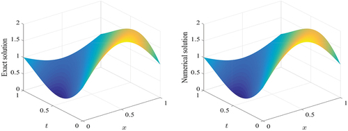
Table 1. Comparison of a new QUICK scheme and existing upwind approach in the FVM for convection dominance case with u = 1 and h = 0.1.

Our scheme		Modified upwind scheme [27]
$\mathrm{\Delta }x$	Max-Error	Max-Error
$t=1/500$
$1/10$	$1.5471\times {10}^{-4}$	$0.0089$
$1/20$	$8.0622\times {10}^{-5}$	$0.0025$
$1/40$	$5.2154\times {10}^{-6}$	$6.8518\times {10}^{-4}$

Example 2.

Consider a convection – diffusion equation (1). An exact solution is given in [27] as follow:

(40) $f(x,t)=\frac{1}{\sqrt{4t+1}}{e}^{\left(-{\left(x-1-ut\right)}^2\right)/h\left(4t+1\right)}.$(40)

The initial and boundary conditions are calculated from eq. (40) by putting $t=0.5$, and $x=1$, $x=2$, respectively.

In the case of convection dominance, Table 2 depicts the comparison of our scheme and existing upwind approaches in the FVM taking the convection coefficient $u=1$ and the diffusion coefficient $h=0.4$. In the case of diffusion dominance, Table 3 shows the comparison of QUICK scheme and existing upwind approaches in the FVM, taking the convection coefficient $u=0.05$ and the diffusion coefficient $h=0.7$. In both reported cases, the result obtained by the quadratic upwind differencing scheme is more accurate compared with the results obtained by the existing upwind schemes in the FVM. For the convection dominance case ($u=1$ and $h=0.02$), Example 2 is approximated using a quadratic upwind differencing scheme in the FVM and the result shown in Figure 4a at $x\in \left[1,2\right]$ and $t\in \left[0.5,1\right]$. Figure 4b is also approximated using a quadratic upwind differencing scheme of the FVM for the convection dominance case ($u=0.7,h=0.02$) at $x\in \left[1,2\right]$ and $t\in \left[0.5,1\right]$.

Figure 4. Mesh plot of solution of example 2 for a. $u=1$, $h=0.02$ and b. $u=0.7$, $h=0.02$.

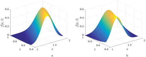
Table 2. Comparison of a QUICK approach and existing upwind techniques in the FVM in the case of convection dominance.

Our scheme		Method in [27]	Method in [54]
$\mathrm{\Delta }x$	Max-Error	Max-Error	Max-Error
$t=1/5000$
$1/10$	$3.1054\times {10}^{-4}$	$0.0038$	$0.0154$
$1/20$	$7.4539\times {10}^{-5}$	$0.0012$	$0.0081$
$1/40$	$2.0673\times {10}^{-6}$	$3.2596\times {10}^{-4}$	$0.0041$
$1/80$	$5.8271\times {10}^{-7}$	$8.7216\times {10}^{-5}$	$0.0021$

Table 3. Comparison of a new QUICK scheme and existing upwind approaches in the FVM taking $u=0.05$ and $h=0.7$ in case of diffusion dominance.

Our scheme		Method in [27]	Method in [54]
$\mathrm{\Delta }x$	Max-Error	Max-Error	Max-error
$t=1/5000$
$1/10$	$1.8205\times {10}^{-4}$	$0.0026$	$0.0124$
$1/20$	$3.9741\times {10}^{-6}$	$7.2459\times {10}^{-4}$	$0.0063$
$1/40$	$9.5383\times {10}^{-7}$	$1.9495\times {10}^{-4}$	$0.0032$
$1/80$	$2.1664\times {10}^{-7}$	$5.4858\times {10}^{-5}$	$0.0016$

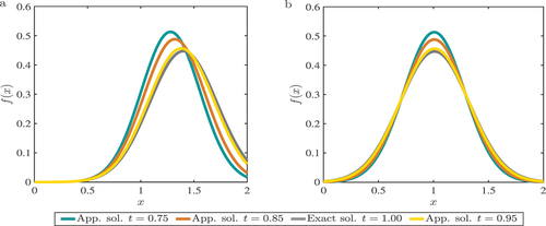
The 2D plot of the solution behaviour of Example 2 with different time levels is plotted in Figure 5. In Figure 5a, the graph indicates approximate results in convection dominant case $u=0.4$ and $h=0.04$; while in Figure 5b, the graph indicates approximate results in diffusion dominant case $u=0.01$ and $h=0.04$ at different time levels. These two figures confirm that the increase of the time level for an approximate results using our proposed scheme to get close to the analytic solution.

Figure 5. Solutions to example 2 for a. $u=0.4$, $h=0.04$; b. $u=0.01$, $h=0.04$.

Example 3.

Consider a convection – diffusion equation (1). The exact solution is found in [27]:

(41) $f(x,t)=\frac{1}{\sqrt{4t+1}}{e}^{\left(-{\left(x-1-ut\right)}^2\right)/h\left(4t+1\right)}.$(41)

The starting and boundary values are computed from eq. (41) by substituting $t=0$, and $x=0$, $x=2$, respectively.

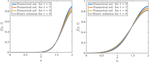
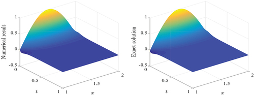
The 3D view of the convection-diffusion approximation over the computational domain $\left(x,t\right)\in \left[0,2\right]\times \left[0,2\right]$ in the FVM of the QUICK scheme at different values of the convection and diffusion coefficients for numerical example 3 are plotted in Figures 6 and 7. Figure 8a shows the numerical result to Example 3 for convection dominance case using a quadratic upwind differencing scheme in the FVM with different time levels. Figure 8b, shows the numerical solution to Example 3 for diffusion dominance case using a quadratic upwind differencing scheme in the FVM with different time levels. Both figures confirm that the increase of the time level for an approximate results using our proposed scheme to get close to the analytic solution.

Figure 6. Mesh plot of solution of example 3 for a. $u=3.2$, $h=0.02$ and b. $u=5$, $h=0.01$.

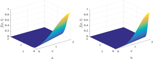
Figure 7. Mesh plot of solution of example 3 for a. $u=1.5$, $h=0.003$ and b. $u=2.5$, $h=0.002$.

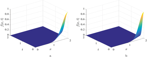
Figure 8. Solutions to example 3 for a. convection dominance $u=0.007$, $h=0.002$ and b. diffusion dominance $u=0.001$, $h=0.005$.

Example 4.

Consider a convection – diffusion equation (1). The exact solution is given in [31] as follow

(42) $f\left(x,t\right)=-sin\left(\pi \left(x-t\right)\right)e^{-2{\pi }^{2}t}.$(42)

The starting and boundary values are computed from eq. (42) by substituting $t=0$, and $x=1$, $x=2$, respectively.

The mesh plot of the solution of Example 4 computed using QUICK scheme and the exact solution is drawn in Figure 9 at $x\in \left[1,2\right]$ and $t\in \left[0,1\right]$ for convection dominance case ($u=0.5$, $h=0.07$) gives maximum absolute error $1.0457\times {10}^{-6}$. This shows that the new scheme provides excellent agreement with the analytic solution. In all tables and figures, the obtained results support our theoretical procedures. From all tables and figures above, the proposed quadratic upwind scheme gives a small maximum error; this indicates that our approximation is highly accurate as compared to the previous approximate techniques.

Figure 9. Exact solution with approximate result of example 4 at $u=0.5$, $h=0.07$.

5. Conclusion

The convection-diffusion equation is one of the most important equation used to represent physical phenomena. Here, we study the approximate assessment of a quadratic upwind differencing approach in the FVM to approximate a convection-diffusion equation (1). In order to numerically approximate convection-diffusion equation with initial and boundary values, a quadratic upwind differencing approach in the FVM is proposed. With the consideration of positive and negative flow directions, new expressions for interface approximations have been obtained for the directional flow phenomenon, and using those approximations, our numerical approach was created with third-order accuracy in space. The temporal integration is approximated using the explicit theta method of first-order accuracy. The method’s stability has been examined, and it has been demonstrated that it is conditionally stable. The equations for different convective velocity ($u$) and diffusion coefficient ($h$) have been approximately calculated by this newly constructed finite volume approach. We successfully showed a numerical comparison of our scheme in the FVM with the previous modified upwind technique and an upwind technique of the FVM. Approximate values have been found using MATLAB R2016a software. From our discussions, we observed that the results of a quadratic upwind differencing scheme are almost indistinguishable from the exact solutions. The approximate values obtained by these numerical schemes show that our newly proposed scheme gives better results and is very close to the analytic result, so this technique gives an additional alternative for solving engineering and science issues. Future work will further investigate by including both Brownian and thermophoresis parameters to the given problem and aiming at further discussion of the scheme’s computational efficiency.

Acknowledgments

The authors express their sincere thanks to the editor and reviewers for their fruitful comments and suggestions that improved the quality of the manuscript.

Disclosure statement

The authors declare that they have no known competing financial interests.

Additional information

Funding

No funding was received for conducting this study.

Appendix

The quadratic upwind differencing scheme in terms of the Taylor series truncation error is third-order accuracy, and its expansion about the east face $f_{i+\frac{\mathrm{\Delta }x}{2},j}$ of the ${\mathrm{i}}^{th}$ control volume gives:

(A1) $f_{i+1,j}=f_{i+\frac{\mathrm{\Delta }x}{2},j}+\frac{1}{2}\mathrm{\Delta }x{\left(\frac{\mathrm{\partial }f}{\mathrm{\partial }x}\right)}_{i+\frac{\mathrm{\Delta }x}{2},j}+\frac{1}{2}{\left(\frac{1}{2}\mathrm{\Delta }{x}^2\right)}^2{\left(\frac{{\mathrm{\partial }}^{2}f}{\mathrm{\partial }{x}^2}\right)}_{i+\frac{\mathrm{\Delta }x}{2},j}+\mathcal{O}\left(\mathrm{\Delta }{x}^3\right).$(A1)

(A2) $f_{i,j}=f_{i+\frac{\mathrm{\Delta }x}{2},j}-\frac{1}{2}\mathrm{\Delta }x{\left(\frac{\mathrm{\partial }f}{\mathrm{\partial }x}\right)}_{i+\frac{\mathrm{\Delta }x}{2},j}+\frac{1}{2}{\left(-\frac{1}{2}\mathrm{\Delta }{x}^2\right)}^2{\left(\frac{{\mathrm{\partial }}^{2}f}{\mathrm{\partial }{x}^2}\right)}_{i+\frac{\mathrm{\Delta }x}{2},j}+\mathcal{O}\left(\mathrm{\Delta }{x}^3\right).$(A2)

(A3) $f_{i-1,j}=f_{i+\frac{\mathrm{\Delta }x}{2},j}-\frac{3}{2}\mathrm{\Delta }x{\left(\frac{\mathrm{\partial }f}{\mathrm{\partial }x}\right)}_{i+\frac{\mathrm{\Delta }x}{2},j}+\frac{1}{2}{\left(-\frac{3}{2}\mathrm{\Delta }{x}^2\right)}^2{\left(\frac{{\mathrm{\partial }}^{2}f}{\mathrm{\partial }{x}^2}\right)}_{i+\frac{\mathrm{\Delta }x}{2},j}+\mathcal{O}\left(\mathrm{\Delta }{x}^3\right).$(A3)

If we add together $\frac{3}{8}\times$eq. (A1) $+\frac{6}{8}\times$eq. (A2)$-\frac{1}{8}\times$eq. (A3) we obtain:

(A4) $f_{i+\frac{\mathrm{\Delta }x}{2},j}=\frac{3}{8}{f}_{i+1,j}+\frac{6}{8}{f}_{i,j}-\frac{1}{8}{f}_{i-1,j}+\mathcal{O}\left(\mathrm{\Delta }{x}^3\right).$(A4)

and eq. (A1)$-$eq. (A2) gives:

(A5) ${\left(\frac{\mathrm{\partial }f}{\mathrm{\partial }x}\right)}_{i+\frac{\mathrm{\Delta }x}{2},j}=\frac{f_{i+1,j}-f_{i,j}}{\mathrm{\Delta }x}+\mathcal{O}\left(\mathrm{\Delta }{x}^3\right).$(A5)

Taylor series expansion about the west face $f_{i-\frac{\mathrm{\Delta }x}{2},j}$ of the ${\mathrm{i}}^{th}$ control volume gives:

(A6) $f_{i,j}=f_{i-\frac{\mathrm{\Delta }x}{2},j}+\frac{1}{2}\mathrm{\Delta }x{\left(\frac{\mathrm{\partial }f}{\mathrm{\partial }x}\right)}_{i-\frac{\mathrm{\Delta }x}{2},j}+\frac{1}{2}{\left(\frac{1}{2}\mathrm{\Delta }{x}^2\right)}^2{\left(\frac{{\mathrm{\partial }}^{2}f}{\mathrm{\partial }{x}^2}\right)}_{i-\frac{\mathrm{\Delta }x}{2},j}+\mathcal{O}\left(\mathrm{\Delta }{x}^3\right).$(A6)

(A7) $f_{i-1,j}=f_{i-\frac{\mathrm{\Delta }x}{2},j}-\frac{1}{2}\mathrm{\Delta }x{\left(\frac{\mathrm{\partial }f}{\mathrm{\partial }x}\right)}_{i-\frac{\mathrm{\Delta }x}{2},j}+\frac{1}{2}{\left(-\frac{1}{2}\mathrm{\Delta }{x}^2\right)}^2{\left(\frac{{\mathrm{\partial }}^{2}f}{\mathrm{\partial }{x}^2}\right)}_{i-\frac{\mathrm{\Delta }x}{2},j}+\mathcal{O}\left(\mathrm{\Delta }{x}^3\right).$(A7)

(A8) $f_{i-2,j}=f_{i-\frac{\mathrm{\Delta }x}{2},j}-\frac{3}{2}\mathrm{\Delta }x{\left(\frac{\mathrm{\partial }f}{\mathrm{\partial }x}\right)}_{i-\frac{\mathrm{\Delta }x}{2},j}+\frac{1}{2}{\left(-\frac{3}{2}\mathrm{\Delta }{x}^2\right)}^2{\left(\frac{{\mathrm{\partial }}^{2}f}{\mathrm{\partial }{x}^2}\right)}_{i-\frac{\mathrm{\Delta }x}{2},j}+\mathcal{O}\left(\mathrm{\Delta }{x}^3\right).$(A8)

If we add together $\frac{3}{8}\times$ eq. (A6) $+\frac{6}{8}\times$ eq. (A7)$-\frac{1}{8}\times$eq. (A8) we obtain:

(A9) $f_{i-\frac{\mathrm{\Delta }x}{2},j}=\frac{3}{8}{f}_{i,j}+\frac{6}{8}{f}_{i-1,j}-\frac{1}{8}{f}_{i-2,j}+\mathcal{O}\left(\mathrm{\Delta }{x}^3\right).$(A9)

and eq. (A6)$-$eq. (A7) gives:

(A10) ${\left(\frac{\mathrm{\partial }f}{\mathrm{\partial }x}\right)}_{i-\frac{\mathrm{\Delta }x}{2},j}=\frac{f_{i,j}-f_{i-1,j}}{\mathrm{\Delta }x}+\mathcal{O}\left(\mathrm{\Delta }{x}^3\right).$(A10)

References

- E. Hernandez-Martinez, H. Puebla, F. Valdes-Parada, and J. Alvarez-Ramirez, Nonstandard finite difference schemes based on Green’s function formulations for reaction–diffusion–convection systems, Chem. Eng. Sci. 94 (2013), pp. 245–255. doi:10.1016/j.ces.2013.03.001.
- J.D. Anderson and J. Wendt, Computational Fluid Dynamics, Vol. 206. Berlin, Heidelberg: Springer, 1995.
- S. Rehman, N. Muhammad, M. Alshehri, S. Alkarni, S.M. Eldin, and N.A. Shah, Analysis of a viscoelastic fluid flow with Cattaneo–Christov heat flux and soret–Dufour effects, Case Stud. Therm. Eng. 49 (2023), pp. 103223. doi:10.1016/j.csite.2023.103223.
- M.N. Ozisik, Heat Transfer: A Basic Approach, McGraw-Hill, New York, 1985.
- N. Muhammad, S. Nadeem, and F.D. Zaman, Transmission of the thermal energy in a ferromagnetic nanofluid flow, Int. J. Mod. Phys. B. 36 (32) (2022). doi:10.1142/S0217979222502368
- N. Naeem, D. Vieru, N. Muhammad, and N. Ahmed, Axial Symmetric Granular Flow Due to Gravity in a Circular Pipe, Symmetry 14 (10) (2022), pp. 1–12. doi:https://doi.org/10.3390/sym14102013.
- J. Philibert, One and a half century of diffusion: Fick, Einstein, before and beyond, Diffus. Fundam 2 (2005), pp. .1.1–.1.10.
- N.M. Buckman, The Linear Convection-Diffusion Equation in Two Dimensions. 18.303 Linear Partial Differential Equations. Cambridge: Massachusetts Institute of Technology, 2016, pp. 1–6.
- M. Usman, A. Hussain, F.D. Zaman, and S.M. Eldin, Group invariant solutions of wave propagation in phononic materials based on the reduced micromorphic model via optimal system of Lie subalgebra, Results Phys 48 (2023), pp. 106413. doi:10.1016/j.rinp.2023.106413.
- S. Rehman, A. Hussain, J.U. Rahman, N. Anjum, and T. Munir, Modified Laplace based variational iteration method for the mechanical vibrations and its applications, acta mechanica et automatica 16 (2) (2022), pp. 98–102. doi:10.2478/ama-2022-0012.
- A. Hussain, A.H. Kara, and F.D. Zaman, An invariance analysis of the vakhnenko–parkes equation, Chaos Solitons Fractals 171 (2023), pp. 113423. doi:https://doi.org/10.1016/j.chaos.2023.113423.
- A. Hussain, M. Usman, F.D. Zaman, and S.M. Eldin, Optical solitons with DNA dynamics arising in oscillator-chain of Peyrard–Bishop model, Results Phys 50 (2023), pp. 106586. doi:10.1016/j.rinp.2023.106586.
- M. Usman, A. Hussain, and F.D. Zaman, Invariance analysis of thermophoretic motion equation depicting the wrinkle propagation in substrate-supported graphene sheets, Phys. Scr. 98 (9) (2023), pp. 095205. doi:https://doi.org/10.1088/1402-4896/acea46.
- A. Hussain, M. Usman, F.D. Zaman, and S.M. Eldin, Symmetry analysis and invariant solutions of Riabouchinsky Proudman Johnson equation using optimal system of Lie subalgebras, Results Phys 49 (2023), pp. 106507. doi:10.1016/j.rinp.2023.106507.
- M. Usman, A. Hussain, F.D. Zaman, I. Khan, and S.M. Eldin, Reciprocal bäcklund transformations and traveling wave structures of some non-linear pseudo-parabolic equations, Partial Differ. Equ. Appl. Math 7 (2023), pp. 100490. doi:10.1016/j.padiff.2023.100490.
- M. Usman and F.D. Zaman, Lie symmetry analysis and conservation laws of non-linear (2+1) elastic wave equation, Arab J. Math 12 (1) (2022), pp. 265–276. doi:10.1007/s40065-022-00392-y.
- H. Okamoto and J. Zhu, Some similarity solutions of the Navier-Stokes equations and related topics, Taiwanese J. Math 4 (1) (2000), pp. 65–103. doi:10.11650/twjm/1500407199.
- F. Moukalled, The Finite Volume Method in Computational Fluid Dynamics, Vol. 113. Cham: Springer, 2016.
- D. Causona, C. Mingham, and L. Qia, Introductory Finite Volume Methods for PDEs, Manchester Metropolitan University, Manchester, UK, 2011.
- F. Moukalled, L. Mangani, and M. Darwish, The Finite Volume Method in Computational Fluid Dynamics, Vol. 6, Springer, Berlin/Heidelberg, Germany, 2016.
- N. Muhammad and K.A.M. Alharbi, OpenFoam for computational hydrodynamics using finite volume method, Int. J. Mod. Phys. B. 37 (3) (2022). doi:10.1142/S0217979223500261
- N. Muhammad and N. Ullah, Simulation of flow on the hydroelectric power dam spillway via OpenFOAM, Eur. Phys. J. Plus. 136 (11) (2021). doi:10.1140/epjp/s13360-021-02128-x
- N. Muhammad, M.M.A. Lashin, and S. Alkhatib, Simulation of turbulence flow in OpenFOAM using the large eddy simulation model, Proc. Inst. Mech. Eng, Part E: J. Process Mech. Eng. 236 (5) (2022), pp. 2252–2265. doi:10.1177/09544089221109736.
- N. Muhammad, S. Ullah, and U. Khan, Energy recovery mechanism of air injection in higher methane cut reservoir, Int. J. Mod. Phys. B. 36 (24) (2022). doi:10.1142/S0217979222501533
- N. Muhammad, F.D. Zaman, and M.T. Mustafa, OpenFOAM for computational combustion dynamics, Eur. Phys. J. Spec. Top 231 (13–14) (2022), pp. 2821–2835. doi:10.1140/epjs/s11734-022-00606-6.
- N. Muhammad, Finite volume method for simulation of flowing fluid via OpenFOAM, Eur. Phys. J. Plus. 136 (10) (2021). doi:10.1140/epjp/s13360-021-01983-y
- A. Hussain, Z. Zheng, and E.F. Anley, Numerical analysis of convection–diffusion using a modified upwind approach in the finite volume method, Math. 8 (1869) (2020), pp. 1–21. doi:10.3390/math8111869.
- Z.F. Tiana and P.X. Yua, A high-order exponential scheme for solving 1D unsteady convection–diffusion equations, J. Comput. Appl. Math. 235 (8) (2011), pp. 2477–2491. doi:10.1016/j.cam.2010.11.001.
- T. Linss, Uniform point-wise convergence of an upwind finite volume method on layer-adapted meshes, Zeitschrift für Angewandte Mathematik und Mechanik 82 (4) (2002), pp. 247–254. doi:10.1002/1521-4001(200204)82:4<247:AID-ZAMM247>3.0.CO;2-9.
- M.R. Patel and J.U. Pandya, A research study on unsteady state convection diffusion flow with the adoption of the finite volume technique, J. Appli. Math. Comput. Mech 20 (4) (2021), pp. 65–76. doi:10.17512/jamcm.2021.4.06.
- R. Edwan, S. Al-Omari, M. Al-Smadi, S. Momani, and A. Fulga, A new formulation of finite difference and finite volume methods for solving a space fractional convection–diffusion model with fewer error estimates, Adv. Differ. Equ 2021 (1) (2021), pp. 510. doi:https://doi.org/10.1186/s13662-021-03669-2.
- ] R. Saadeh, Numerical solutions of fractional convection-diffusion equation using finite-difference and finite-volume schemes, J. Math. Comput. Sci. 11, 6 (2021), pp. 1927–5307. doi:10.28919/jmcs/6658
- M.R. Patel and J.U. Pandya, Numerical study of a one and two-dimensional heat flow using finite volume, Mater. Today Proc. 10.1016/j.matpr.2021.04.413.
- J. Nakao, J. Chen, and J.M. Qiu, An Eulerian-Lagranian Runge-Kutta finite volume (EL-RK-FV) method for solving convection and convection-diffusion equation, J. Comput. Phys. 470 (2022), pp. 111589. doi:10.1016/j.jcp.2022.111589.
- C. Chainais-Hillairet and M. Herda, Large-time behaviour of a family of finite volume schemes for boundary-driven convection-diffusion equations, IMA J. Numer. Anal 40 (4) (2020), pp. 2473–2504. doi:10.1093/imanum/drz037.
- I. Asmouh, M. El-Amrani, M. Seaid, and N. Yebari, A conservative semi-Lagrangian finite volume method for convection–diffusion problems on unstructured grids, J. Sci. Comput 85 (1) (2020), pp. 11. doi:https://doi.org/10.1007/s10915-020-01316-8.
- M. Xu, A finite volume scheme for unsteady linear and nonlinear convection-diffusion-reaction problems, Int. Commun. Heat Mass Transf 139 (2022), pp. 106417. doi:10.1016/j.icheatmasstransfer.2022.106417.
- E.F. Anley and Z. Zheng, Finite difference approximation method for a space fractional convection-diffusion equation with variable coefficients, Symmetry 12 (3) (2020), pp. 485. doi:10.3390/sym12030485.
- H.F. Peng, K. Yang, M. Cui, and X.W. Gao, Radial integration boundary element method for solving two-dimensional unsteady convection-diffusion problem, Eng. Anal. Bound. Elem. 102 (2019), pp. 39–50. doi:10.1016/j.enganabound.2019.01.019.
- V. Aswin, A. Awasthi, and C. Anu, A comparative study of numerical schemes for convection-diffusion equation, Procedia. Eng 127 (2015), pp. 621–627. doi:10.1016/j.proeng.2015.11.353.
- M. Xu, A modified finite volume method for convection-diffusion-reaction problems, Int. J. Heat Mass Tran. 117 (2018), pp. 658–668. doi:10.1016/j.ijheatmasstransfer.2017.10.003.
- M.T. Xu, A type of high order schemes for steady convection-diffusion problems, Int. J. Heat Mass. Transf. 107:1044–1053, (2017).
- R. Mohammadi, Exponential B–Spline solution of convection-Diffusion equations, Appl. Math. 4 (6) (2013), pp. 933–944. doi:10.4236/am.2013.46129.
- B.P. Leonard, A stable and accurate convective modelling procedure based on quadratic upstream interpolation, Comput. Methods Appl. Mech. Eng. 19 (1) (1979), pp. 59–98. doi:10.1016/0045-7825(79)90034-3.
- J. Fuhrmann, M. Ohlberger, and C. Rohde, Finite Volumes for Complex Applications VII: Methods and Theoretical Aspects, Vol. 77, Springer; FVCA, Berlin, Germany, 2014.
- J. Mencinger, Numerical simulation of melting in two-dimensional cavity using adaptive grid, J. Comput. Phys. 198 (1) (2004), pp. 243–264. doi:10.1016/j.jcp.2004.01.006.
- E.J. Sellountos, A single domain velocity - vorticity Fast Multipole Boundary Domain Element Method for three dimensional incompressible fluid flow problems, Eng. Anal. Bound. Elem. 114 (2020), pp. 74–93. doi:10.1016/j.enganabound.2020.02.006.
- P. Pathmanathan, M.O. Bernabeu, R. Bordas, J. Cooper, A. Garny, J.M. Pitt-Francis, J.P. Whiteley, and D.J. Gavaghan, A numerical guide to the solution of the bidomain equations of cardiac electrophysiology, Prog. Biophys. Mol. Biol. 102 (2–3) (2010), pp. 136–155. doi:10.1016/j.pbiomolbio.2010.05.006.
- Y. Coudière, C. Pierre, O. Rousseau, and R. Turpault, A 2D/3D discrete duality finite volume scheme, Application to ECG simulation, Int. J. Finite 6 (2009), pp. 1–24.
- P.R. Johnston, A finite volume method solution for the bidomain equations and their application to modelling cardiac ischaemia, Comput. Methods Biomech. Biomed. Eng. 13 (2) (2010), pp. 157–170. http://dx.doi.org/10.1080/10255840903067072
- T. Munir, Analysis of coupling interface problems for bi-domain diffusion equations, 2020 Ph.D. thesis.
- H.K. Versteeg and W. Malalasekera, An Introduction to Computational Fluid Dynamics: The Finite Volume Method, Pearson Education, Edinburgh, UK, 2007. www.pearsoned.co.uk/versteeg.
- R.D. Richtmyer and K.W. Morton, Difference Methods for Initial-Value Problems, Intencience, New York, 1967.
- G.G. Botte, J.A. Ritter, and R.E. White, Comparison of finite difference and control volume methods for solving differential equations, Comput. Chem. Eng. 24 (12) (2000), pp. 2633–2654. doi:10.1016/S0098-1354(00)00619-0.