Probabilistic degenerate Bernoulli and degenerate Euler polynomials

ABSTRACT

Recently, many authors have studied degenerate Bernoulli and degenerate Euler polynomials. Let $\mathit{Y}$ be a random variable whose moment generating function exists in a neighbourhood of the origin. The aim of this paper is to introduce and study the probabilistic extension of degenerate Bernoulli and degenerate Euler polynomials, namely the probabilistic degenerate Bernoulli polynomials associated with $\mathit{Y}$ and the probabilistic degenerate Euler polynomials associated with $\mathit{Y}$. Also, we intoduce the probabilistic degenerate $\mathit{r}$-Stirling numbers of the second associated with $\mathit{Y}$ and the probabilistic degenerate two variable Fubini polynomials associated with $\mathit{Y}$. We obtain some properties, explicit expressions, recurrence relations and certain identities for those polynomials and numbers. As special cases of $\mathit{Y}$, we treat the gamma random variable with parameters $\mathit{\alpha },\mathit{\beta }>0$, the Poisson random variable with parameter $\mathit{\alpha }>0$, and the Bernoulli random variable with probability of success $\mathit{p}$.

MATHEMATICS SUBJECT CLASSIFICATION:

• 11B68
• 11B73
• 11B83

KEYWORDS:

• Probabilistic degenerate Bernoulli polynomials
• prob- abilistic degenerate Euler polynomials
• gamma random variable

1. Introduction

In [1], Carlitz initiated a study of degenerate versions of Bernoulli and Euler polynomials, namely the degenerate Bernoulli and degenerate Euler polynomials. In recent years, a lot of work has been done for various degenerate versions of many special polynomials and numbers. For example, we found the degenerate Stirling numbers of the first kind and the second kind which turned out to be very important in studying degenerate versions of special polynomials and numbers. It is also remarkable that degenerate umbral calculus and degenerate gamma function were developed along the way.

Let $\mathit{Y}$ be a random variable satisfying the moment condition (see (13)). The aim of this paper is to study, as probabilistic extensions of degenerate Bernoulli and degenerate Euler polynomials, the probabilistic degenerate Bernoulli polynomials associated with $\mathit{Y}$ and the probabilistic degenerate Euler polynomials associated with $\mathit{Y}$, along with the probabilistic degenerate $\mathit{r}$-Stirling numbers of the second kind associated with $\mathit{Y}$ and the probabilistic degenerate two variable Fubini polynomials associated with $\mathit{Y}$.

We derive some properties, explicit expressions, certain identities and recurrence relations for those polynomials and numbers. In addition, as special cases of $\mathit{Y}$, we consider the gamma random variable with parameters $\mathit{\alpha },\mathit{\beta }>0$, the Poisson random variable with parameter $\mathit{\alpha }>0$, and the Bernoulli random variable with probability of success $\mathit{p}$.

The outline of this paper is as follows. In Section 1, we recall the degenerate exponentials, the degenerate Bernoulli polynomials and the degenerate Euler polynomials. We remind the reader of the degenerate Stirling numbers of the first and the second kinds, and the degenerate $\mathit{r}$-Stirling numbers of the second kind. We recall the degenerate Fubini polynomials and the degenerate two variable Fubini polynomials. Assume that $\mathit{Y}$ is a random variable such that the moment generating function of $\mathit{Y}$, $\mathit{E}[e^{\mathit{tY}}]={\sum }_{n=0}^{\mathrm{\infty }}\frac{t^n}{\mathit{n}!}\mathit{E}[Y^n],(|\mathit{t}|<\mathit{r})$, exists for some $\mathit{r}>0$. Let $(Y_j{)}_{\mathit{j}\ge 1}$ be a sequence of mutually independent copies of the random variable $\mathit{Y}$, and let $S_k=Y_1+Y_2+\cdots +Y_k,(\mathit{k}\ge 1)$, with $S_0=0$. Then we recall the probabilistic degenerate Stirling numbers of the second kind associated with $\mathit{Y}$, ${\left\{\begin{array}{c}\mathit{n}\\ \mathit{k}\end{array}\right\}}_{\mathit{Y},\mathit{\lambda }}$ and the probabilistic degenerate two variable Fubini polynomials associated with $\mathit{Y}$, $F_{n,\lambda }^Y(\mathit{x}|\mathit{y})$. Section 2 includes the main results of this paper. Let $(Y_j{)}_{\mathit{j}\ge 1},S_k,(\mathit{k}=0,1,\dots )$ be as in the above. We define the probabilistic degenerate Bernoulli polynomials associated with $\mathit{Y}$, ${\beta }_{n,\lambda }^Y(\mathit{x})$ (see (21)). Then we find explicit expressions for those polynomials in Theorems 1, 2 and 6. We get respectively in Theorems 3, 4 and 5 probabilistic degenerate analogues, involving ${\beta }_{n,\lambda }^Y(\mathit{x})$ and ${\beta }_{n,\lambda }^Y=:{\beta }_{n,\lambda }^Y(0)$, of the well-known identities for Bernoulli numbers and polynomials, namely ${\sum }_{k=0}^n{k}^m=\frac{1}{\mathit{m}+1}\left\{B_{\mathit{m}+1}(\mathit{n}+1)-B_{\mathit{m}+1}\right\},(\mathit{n},\mathit{m}\ge 0)$, ${\sum }_{l=0}^n\left(\begin{array}{c}\mathit{n}\\ \mathit{l}\end{array}\right)B_l-B_n={\delta }_{\mathit{n},1},(\mathit{n}\ge 0)$, and $B_n=d^{\mathit{n}-1}{\sum }_{k=0}^{d-1}{B}_n(\frac{k}{d}),(\mathit{n}\ge 0,\mathit{d}\ge 1)$. Here ${\delta }_{\mathit{n},1}$ is the Kronecker’s delta so that it is 1 if $\mathit{n}=1$ and 0 otherwise. We determine ${\beta }_{n,\lambda }^Y$ when $\mathit{Y}$ is the gamma random variable with parameters $\mathit{\alpha }=\mathit{\beta }=1$ (see (19)) in Theorem 8 and the Bernoulli random variable with probability of success $\mathit{p}$ in Theorem 9. In Theorem 7, we obtain an identity involving ${\left\{\begin{array}{c}\mathit{n}\\ \mathit{k}\end{array}\right\}}_{\mathit{Y},\mathit{\lambda }}$ and ${\beta }_{m,\lambda }^Y$. Then we define the probabilistic degenerate $\mathit{r}$-Stirling numbers of the second kind associated with $\mathit{Y}$, ${\left\{\begin{array}{c}n+r\\ k+r\end{array}\right\}}_{r,\lambda }^Y$ and obtain an expression for them in Theorem 10. In Theorem 13, we derive a generalization of the identity in Theorem 7 which involves ${\left\{\begin{array}{c}n+r\\ k+r\end{array}\right\}}_{r,\lambda }^Y$ and ${\beta }_m^Y(\mathit{r})$. We deduce an explicit expression for $F_{n,\lambda }^Y(\mathit{x}|\mathit{y})$ in Theorem 11 and that for $F_{n,\lambda }^Y(\mathit{x}|\mathit{r})$, ($\mathit{r}\in \mathbb{Z}$ with $\mathit{r}\ge 0$), in Theorem 12. We define the probabilistic degenerate Euler polynomials associated with $\mathit{Y}$, ${\mathcal{E}}_{n,\lambda }^Y(\mathit{x})$ (see (45)). We find an explicit expression for ${\mathcal{E}}_{n,\lambda }^Y(\mathit{x})$ in Theorem 14 and that for ${\mathcal{E}}_{n,\lambda }^Y={\mathcal{E}}_{n,\lambda }^Y(0)$ in Theorem 15. In Theorem 16, we obtain a probabilistic degenerate analogue, involving ${\mathcal{E}}_{n,\lambda }^Y(\mathit{x})$ and ${\mathcal{E}}_{n,\lambda }^Y$, of the well-known identity for Euler numbers and polynomials, namely ${\sum }_{k=0}^n(-1{)}^k{k}^m=\frac{E_m+E_m(\mathit{n}+1)}{2}$, for any even positive integer $\mathit{n}$. We derive an explicit expression for ${\mathcal{E}}_{n,\lambda }^Y$ when $\mathit{Y}$ is the gamma random variable with parameters $\mathit{\alpha }=\mathit{\beta }=1$ in Theorem 17 and that for ${\mathcal{E}}_{n,\lambda }^Y(\mathit{x})$ when $\mathit{Y}$ is the Poisson random variable with parameter $\mathit{\alpha }>0$ in Theorem 18. For the rest of this section, we recall the facts that are needed throughout this paper.

For any nonzero $\mathit{\lambda }\in \mathbb{R}$, the degenerate exponentials are defined by

(1) $e_{\lambda }^x(\mathit{t})=\sum _{\mathit{k}=0}^{\mathrm{\infty }}\frac{{(\mathit{x})}_{\mathit{k},\mathit{\lambda }}}{\mathit{k}!}{t}^k,e_{\lambda }(\mathit{t})=e_{\lambda }^1(\mathit{t}),(\mathrm{see}[\text{booklink}="\mathrm{cit}0001"1-\text{booklink}="\mathrm{cit}0028"28]),$(1)

where

$(\mathit{x}{)}_{0,\mathit{\lambda }}=1,(\mathit{x}{)}_{\mathit{n},\mathit{\lambda }}=\mathit{x}(\mathit{x}-\mathit{\lambda })(\mathit{x}-2\mathit{\lambda })\cdots (\mathit{x}-(\mathit{n}-1)\mathit{\lambda }),(\mathit{n}\ge 1).$

Carlitz considered the degenerate Bernoulli polynomials defined by

(2) $\frac{t}{e_{\lambda }(\mathit{t})-1}{e}_{\lambda }^x(\mathit{t})=\sum _{\mathit{n}=0}^{\mathrm{\infty }}{\beta }_{\mathit{n},\mathit{\lambda }}(\mathit{x})\frac{t^n}{\mathit{n}!},(\mathrm{see}[\text{booklink}="\mathit{cit}0001"1,\text{booklink}="\mathit{cit}0008"8,\text{booklink}="\mathit{cit}0018"18]).$(2)

When $\mathit{x}=0$, ${\beta }_{\mathit{n},\mathit{\lambda }}={\beta }_{\mathit{n},\mathit{\lambda }}(0)$ are called the degenerate Bernoulli numbers. It is immediate to see from (2) that

(3) ${\beta }_{\mathit{n},\mathit{\lambda }}(\mathit{x})=\sum _{\mathit{k}=0}^n\left(\begin{array}{c}\mathit{n}\\ \mathit{k}\end{array}\right){\beta }_{\mathit{k},\mathit{\lambda }}(\mathit{x}{)}_{\mathit{n}-\mathit{k},\mathit{\lambda }}.$(3)

Note that ${lim}_{\mathit{\lambda }\to 0}{\beta }_{\mathit{n},\mathit{\lambda }}(\mathit{x})=B_n(\mathit{x}),(\mathit{n}\ge 0)$, where $B_n(\mathit{x})$ are the ordinary Bernoulli polynomials given by

$\frac{t}{e^t-1}{e}^{\mathit{xt}}=\sum _{\mathit{n}=0}^{\mathrm{\infty }}{B}_n(\mathit{x})\frac{t^n}{\mathit{n}!},(\mathrm{see}[\text{booklink}="\mathit{cit}0001"1-\text{booklink}="\mathit{cit}0032"32]).$

The degenerate Euler polynomials are defined as

(4) $\frac{2}{e_{\lambda }(\mathit{t})+1}{e}_{\lambda }^x(\mathit{t})=\sum _{\mathit{n}=0}^{\mathrm{\infty }}{\mathcal{E}}_{\mathit{n},\mathit{\lambda }}(\mathit{x})\frac{t^n}{\mathit{n}!},(\mathrm{see}[\text{booklink}="\mathit{cit}0001"1,\text{booklink}="\mathit{cit}0013"13,\text{booklink}="\mathit{cit}0014"14,\text{booklink}="\mathit{cit}0018"18]).$(4)

When $\mathit{x}=0$, ${\mathcal{E}}_{\mathit{n},\mathit{\lambda }}={\mathcal{E}}_{\mathit{n},\mathit{\lambda }}(0)$ are called the degenerate Euler numbers. The values of ${\mathcal{E}}_{\mathit{n},\mathit{\lambda }}$ can be determined from the recurrence relation (see (Kim et al. 23)):

(5) $\sum _{\mathit{k}=0}^{\mathit{n}-1}\left(\begin{array}{c}\mathit{n}\\ \mathit{k}\end{array}\right)(1{)}_{\mathit{n}-\mathit{k},\mathit{\lambda }}{\mathcal{E}}_{\mathit{k},\mathit{\lambda }}+2{\mathcal{E}}_{\mathit{n},\mathit{\lambda }}=0,(\mathit{n}\ge 1),{\mathcal{E}}_{0,\mathit{\lambda }}=1.$(5)

We readily see from (4) that

(6) ${\mathcal{E}}_{\mathit{n},\mathit{\lambda }}(\mathit{x})=\sum _{\mathit{k}=0}^n\left(\begin{array}{c}\mathit{n}\\ \mathit{k}\end{array}\right){\mathcal{E}}_{\mathit{k},\mathit{\lambda }}(\mathit{x}{)}_{\mathit{n}-\mathit{k},\mathit{\lambda }}.$(6)

Note that ${lim}_{\mathit{\lambda }\to 0}{\mathcal{E}}_{\mathit{n},\mathit{\lambda }}(\mathit{x})=E_n(\mathit{x})$, where $E_n(\mathit{x})$ are the ordinary Euler polynomials given by

$\frac{2}{e^t+1}{e}^{\mathit{xt}}=\sum _{\mathit{n}=0}^{\mathrm{\infty }}{E}_n(\mathit{x})\frac{t^n}{\mathit{n}!},(\mathrm{see}[\text{booklink}="\mathit{cit}0003"3,\text{booklink}="\mathit{cit}0024"24,\text{booklink}="\mathit{cit}0025"25,\text{booklink}="\mathit{cit}0029"29]).$

It is well known that the Stirling numbers of the first kind are defined as

(7) $(\mathit{x}{)}_n=\sum _{\mathit{k}=0}^n{S}_1(\mathit{n},\mathit{k})x^k,(\mathit{n}\ge 0),(\mathrm{see}[\text{booklink}="\mathit{cit}0003"3,\text{booklink}="\mathit{cit}0012"12,\text{booklink}="\mathit{cit}0017"17,\text{booklink}="\mathit{cit}0025"25]),$(7)

where

$(\mathit{x}{)}_0=1,(\mathit{x}{)}_n=\mathit{x}(\mathit{x}-1)(\mathit{x}-2)\cdots (\mathit{x}-\mathit{n}+1),(\mathit{n}\ge 1).$

As the inversion formula of (7), the Stirling numbers of the second kind are given by

(8) $x^n=\sum _{\mathit{k}=0}^n\left\{\begin{array}{c}\mathit{n}\\ \mathit{k}\end{array}\right\}(\mathit{x}{)}_k,(\mathit{n}\ge 0),(\mathrm{see}[\text{booklink}="\mathit{cit}0003"3,\text{booklink}="\mathit{cit}0011"11,\text{booklink}="\mathit{cit}0012"12,\text{booklink}="\mathit{cit}0017"17,\text{booklink}="\mathit{cit}0025"25]).$(8)

The degenerate Stirling numbers of the second kind are defined by

(9) $(\mathit{x}{)}_{\mathit{n},\mathit{\lambda }}=\sum _{\mathit{k}=0}^n{\left\{\begin{array}{c}n\\ k\end{array}\right\}}_{\lambda }(\mathit{x}{)}_k,(\mathit{n}\ge 0),(\mathrm{see}[\text{booklink}="\mathit{cit}0008"8]).$(9)

Note that $\underset{\mathit{\lambda }\to 0}{lim}{\left\{\begin{array}{c}n\\ k\end{array}\right\}}_{\lambda }=\left\{\begin{array}{c}\mathit{n}\\ \mathit{k}\end{array}\right\},(\mathit{n}\ge \mathit{k}\ge 0)$. The values of ${\left\{\begin{array}{c}n\\ k\end{array}\right\}}_{\lambda },(\mathit{n}\ge \mathit{k}\ge 0)$ can be determined from the following recurrence relations (see (Kim and Kim 14)):

(10) ${\left\{\begin{array}{c}n+1\\ k\end{array}\right\}}_{\lambda }={\left\{\begin{array}{c}n\\ k-1\end{array}\right\}}_{\lambda }+(\mathit{k}-\mathit{n\lambda }){\left\{\begin{array}{c}n\\ k\end{array}\right\}}_{\lambda },(1\le \mathit{k}\le \mathit{n}),$(10)

${\left\{\begin{array}{c}n\\ n\end{array}\right\}}_{\lambda }=1,(\mathit{n}\ge 0),{\left\{\begin{array}{c}n\\ 0\end{array}\right\}}_{\lambda }=0,(\mathit{n}\ge 1).$

Also, the degenerate Stirling numbers of the first kind are defined by

(11) $(\mathit{x}{)}_n=\sum _{\mathit{k}=0}^n{S}_{1,\mathit{\lambda }}(\mathit{n},\mathit{k})(\mathit{x}{)}_{\mathit{k},\mathit{\lambda }},(\mathit{n}\ge 0),(\mathrm{see}[\text{booklink}="\mathit{cit}0008"8]).$(11)

From (9), we can easily see that

$\sum _{\mathit{k}=1}^n{\lambda }^{\mathit{k}-1}(1{)}_{\mathit{k},1/\lambda }{\left\{\begin{array}{c}n\\ k\end{array}\right\}}_{\lambda }={\delta }_{1,\mathit{n}},(\mathit{n}\in \mathbb{N}),$

where ${\delta }_{\mathit{n},\mathit{k}}$ is Kronecker's symbol.

Let $\mathit{r}$ be a nonnegative integer. Then the degenerate $\mathit{r}$-Stirling numbers of the second kind are defined by

(12) $(\mathit{x}+\mathit{r}{)}_{\mathit{n},\mathit{\lambda }}=\sum _{\mathit{k}=0}^n{\left\{\begin{array}{c}n+r\\ k+r\end{array}\right\}}_{\mathit{r},\mathit{\lambda }}(\mathit{x}{)}_k,(\mathit{n}\ge 0),(\mathrm{see}[\text{booklink}="\mathit{cit}0012"12,\text{booklink}="\mathit{cit}0015"15,\text{booklink}="\mathit{cit}0017"17]).$(12)

From (12), we note that

(13) $\frac{1}{\mathit{k}!}{(e_{\lambda }(\mathit{t})-1)}^{\mathit{k}}{e}_{\lambda }^r(\mathit{t})={\displaystyle \sum _{\mathit{n}=\mathit{k}}^{\infty }{\left\{\begin{array}{l}\mathit{n}+\mathit{r}\\ \mathit{k}+\mathit{r}\end{array}\right\}}_{\mathit{r},\mathit{\lambda }}\frac{t^n}{\mathit{n}!},}$(13)

where $\mathit{k}$ is a nonnegative integer.

The degenerate Fubini polynomials are given by

(14) $\frac{1}{1-x(e_{\lambda }(\mathit{t})-1)}=\sum _{\mathit{n}=0}^{\mathrm{\infty }}{F}_{\mathit{n},\mathit{\lambda }}(\mathit{x})\frac{t^n}{\mathit{n}!},(\mathrm{see}[\text{booklink}="\mathit{cit}0018"18]).$(14)

Thus, by (14), we get

(15) $F_{\mathit{n},\mathit{\lambda }}(\mathit{x})=\sum _{\mathit{k}=0}^n{x}^k{\left\{\begin{array}{c}n\\ k\end{array}\right\}}_{\lambda }\mathit{k}!,(\mathit{n}\ge 0),(\mathrm{see}[\text{booklink}="\mathit{cit}0018"18]).$(15)

The degenerate two variable Fubini polynomials are defined by

(16) $\frac{1}{1-x(e_{\lambda }(\mathit{t})-1)}{e}_{\lambda }^y(\mathit{t})=\sum _{\mathit{n}=0}^{\mathrm{\infty }}{F}_{\mathit{n},\mathit{\lambda }}(\mathit{x}|\mathit{y})\frac{t^n}{\mathit{n}!}.$(16)

Note that $F_{\mathit{n},\mathit{\lambda }}(\mathit{x}|0)=F_{\mathit{n},\mathit{\lambda }}(\mathit{x}),(\mathit{n}\ge 0)$.

Assume that $\mathit{Y}$ is a random variable such that the moment generating function of $\mathit{Y}$

(17) $\mathit{E}[e^{\mathit{tY}}]=\sum _{\mathit{n}=0}^{\mathrm{\infty }}\mathit{E}[Y^n]\frac{t^n}{\mathit{n}!},(|\mathit{t}|<\mathit{r}),\mathrm{exists}\mathrm{for}\mathrm{some}\mathrm{r}>0,$(17)

where $\mathit{E}$ stands for the mathematical expectation.

Let $(Y_k{)}_{\mathit{k}\ge 1}$ be a sequence of mutually independent copies the random variable $\mathit{Y}$, and let $S_k=Y_1+\cdots +Y_k,(\mathit{k}\ge 1)$ with $S_0=0$.

The probabilistic degenerate Stirling numbers of the second kind associated with $\mathit{Y}$ are defined by

$\frac{1}{\mathit{k}!}(\mathit{E}[e_{\lambda }^Y(\mathit{t})]-1{)}^k=\sum _{\mathit{n}=\mathit{k}}^{\mathrm{\infty }}{\left\{\begin{array}{c}n\\ k\end{array}\right\}}_{\mathit{Y},\mathit{\lambda }}\frac{t^n}{\mathit{n}!},(\mathrm{see}[\text{booklink}="\mathit{cit}0010"10]).$

Note that ${\left\{\begin{array}{c}n\\ k\end{array}\right\}}_{\mathit{Y},\mathit{\lambda }}={\left\{\begin{array}{c}n\\ k\end{array}\right\}}_{\lambda }$ if $\mathit{Y}=1$.

Recently, the probabilistic degenerate two variable Fubini polynomials associated with $\mathit{Y}$ are given by

(18) $\frac{1}{1-x(E[e_{\lambda }^Y(\mathit{t})]-1)}(\mathit{E}[e_{\lambda }^Y(\mathit{t})]{)}^y=\sum _{\mathit{n}=0}^{\mathrm{\infty }}{F}_{n,\lambda }^Y(\mathit{x}|\mathit{y})\frac{t^n}{\mathit{n}!},(\mathrm{see}[\text{booklink}="\mathit{cit}0028"28,\text{booklink}="\mathit{cit}0034"34]).$(18)

When $\mathit{y}=0$, $F_{n,\lambda }^Y(\mathit{x})=F_{n,\lambda }^Y(\mathit{x}|0)$ are called the probabilistic degenerate Fubini polynomials associated with $\mathit{Y}$.

2. Probabilistic degenerate Bernoulli and degenerate Euler polynomials

A continuous random variable $\mathit{Y}$ whose density function is given by

(19) $\mathit{f}(\mathit{y})=\left\{\begin{array}{ccc}\mathit{\beta }{e}^{-\mathit{\beta y}}\frac{{(\mathit{\beta y})}^{\mathit{\alpha }-1}}{\mathrm{\Gamma }(\mathit{\alpha })},& \mathrm{if}\mathit{y}\ge 0,& \mathit{\hspace{0.17em}}\\ 0,& \mathrm{if}\mathit{y}<0,& \mathit{\hspace{0.17em}}\end{array}\right.$(19)

for some $\mathit{\alpha },\mathit{\beta }>0$ is said to be the gamma random variable with parameters $\mathit{\alpha },\mathit{\beta }$, which is denoted by $\mathit{Y}\sim \mathrm{\Gamma }(\mathit{\alpha },\mathit{\beta })$, (see (Leon-Garcia 26; Simsek 33)).

Let $(Y_k{)}_{\mathit{k}\ge 1}$ be a sequence of mutually independent copies of random variable $\mathit{Y}$, and let

(20) $S_0=0,S_k=Y_1+Y_2+\cdots +Y_k,(\mathit{k}\ge 1).$(20)

We define the probabilistic degenerate Bernoulli polynomials associated with $\mathit{Y}$ by

(21) $\frac{t}{E[e_{\lambda }^Y(\mathit{t})]-1}(\mathit{E}[e_{\lambda }^Y(\mathit{t})]{)}^x=\sum _{\mathit{n}=0}^{\mathrm{\infty }}{\beta }_{n,\lambda }^Y(\mathit{x})\frac{t^n}{\mathit{n}!}.$(21)

When $\mathit{Y}=1$, ${\beta }_{n,\lambda }^Y(\mathit{x})={\beta }_{\mathit{n},\mathit{\lambda }}(\mathit{x}),(\mathit{n}\ge 0)$.

For $\mathit{x}=0$, ${\beta }_{n,\lambda }^Y={\beta }_{n,\lambda }^Y(0)$ are called the probabilistic degenerate Bernoulli numbers associated with $\mathit{Y}$.

From (21), we note that

(22) $\sum _{\mathit{n}=0}^{\mathrm{\infty }}{\beta }_{n,\lambda }^Y(\mathit{x})\frac{t^n}{\mathit{n}!}=\frac{t}{E[e_{\lambda }^Y(\mathit{t})]-1}(\mathit{E}[e_{\lambda }^Y(\mathit{t})]-1+1{)}^x$(22)

$=\frac{t}{E[e_{\lambda }^Y(\mathit{t})]-1}+\mathit{t}\sum _{\mathit{k}=1}^{\mathrm{\infty }}\left(\begin{array}{c}\mathit{x}\\ \mathit{k}\end{array}\right)(\mathit{E}[e_{\lambda }^Y(\mathit{t})]-1{)}^{\mathit{k}-1}$

$=\frac{t}{E[e_{\lambda }^Y(\mathit{t})]-1}+\mathit{t}\sum _{\mathit{k}=0}^{\mathrm{\infty }}\frac{{(\mathit{x})}_{\mathit{k}+1}}{\mathit{k}+1}\frac{1}{\mathit{k}!}(\mathit{E}[e_{\lambda }^Y(\mathit{t})]-1{)}^k$

$=\sum _{\mathit{n}=0}^{\mathrm{\infty }}{\beta }_{n,\lambda }^Y\frac{t^n}{\mathit{n}!}+\mathit{t}\sum _{\mathit{k}=0}^{\mathrm{\infty }}\frac{{(\mathit{x})}_{\mathit{k}+1}}{\mathit{k}+1}\sum _{\mathit{n}=\mathit{k}}^{\mathrm{\infty }}{\left\{\begin{array}{c}n\\ k\end{array}\right\}}_{\mathit{Y},\mathit{\lambda }}\frac{t^n}{\mathit{n}!}$

$=\sum _{\mathit{n}=0}^{\mathrm{\infty }}{\beta }_{n,\lambda }^Y\frac{t^n}{\mathit{n}!}+\mathit{t}\sum _{\mathit{n}=0}^{\mathrm{\infty }}\sum _{\mathit{k}=0}^n\frac{{(\mathit{x})}_{\mathit{k}+1}}{\mathit{k}+1}{\left\{\begin{array}{c}n\\ k\end{array}\right\}}_{\mathit{Y},\mathit{\lambda }}\frac{t^n}{\mathit{n}!}$

$=\sum _{\mathit{n}=0}^{\mathrm{\infty }}{\beta }_{n,\lambda }^Y\frac{t^n}{\mathit{n}!}+\sum _{\mathit{n}=1}^{\mathrm{\infty }}\mathit{n}\sum _{\mathit{k}=0}^{\mathit{n}-1}\frac{{(\mathit{x})}_{\mathit{k}+1}}{\mathit{k}+1}{\left\{\begin{array}{c}n-1\\ k\end{array}\right\}}_{\mathit{Y},\mathit{\lambda }}\frac{t^n}{\mathit{n}!}.$

Thus, by (22), we get

(23) $\sum _{\mathit{n}=1}^{\mathrm{\infty }}({\beta }_{n,\lambda }^Y(\mathit{x})-{\beta }_{n,\lambda }^Y)\frac{t^n}{\mathit{n}!}=\sum _{\mathit{n}=1}^{\mathrm{\infty }}\mathit{n}\sum _{\mathit{k}=0}^{\mathit{n}-1}\frac{{(\mathit{x})}_{\mathit{k}+1}}{\mathit{k}+1}{\left\{\begin{array}{c}n-1\\ k\end{array}\right\}}_{\mathit{Y},\mathit{\lambda }}\frac{t^n}{\mathit{n}!}.$(23)

Thus, by comparing the coefficients on both sides of (23), we obtain the following theorem.

Theorem 1

For $\mathit{n}\in \mathbb{N}$, we have

$\frac{{\beta }_{n,\lambda }^Y(\mathit{x})-{\beta }_{n,\lambda }^Y}{\mathit{n}}=\sum _{\mathit{k}=0}^{\mathit{n}-1}\frac{{(\mathit{x})}_{\mathit{k}+1}}{\mathit{k}+1}{\left\{\begin{array}{c}n-1\\ k\end{array}\right\}}_{\mathit{Y},\mathit{\lambda }}.$

By binomial expansion, we have

(24) $(\mathit{E}[e_{\lambda }^Y(\mathit{t})]{)}^x=(\mathit{E}[e_{\lambda }^Y(\mathit{t})]-1+1{)}^x=\sum _{\mathit{k}=0}^{\mathrm{\infty }}(\mathit{x}{)}_k\frac{1}{\mathit{k}!}(\mathit{E}[e_{\lambda }^Y(\mathit{t})]-1{)}^k$(24)

$=\sum _{\mathit{k}=0}^{\mathrm{\infty }}(\mathit{x}{)}_k\sum _{\mathit{m}=\mathit{k}}^{\mathrm{\infty }}{\left\{\begin{array}{c}m\\ k\end{array}\right\}}_{\mathit{Y},\mathit{\lambda }}\frac{t^m}{\mathit{m}!}$

$=\sum _{\mathit{m}=0}^{\mathrm{\infty }}(\sum _{\mathit{k}=0}^m{\left\{\begin{array}{c}m\\ k\end{array}\right\}}_{\mathit{Y},\mathit{\lambda }}(\mathit{x}{)}_k)\frac{t^m}{\mathit{m}!}.$

Thus, by (21) and (24), we get

(25) $\sum _{\mathit{n}=0}^{\mathrm{\infty }}{\beta }_{n,\lambda }^Y(\mathit{x})\frac{t^n}{\mathit{n}!}=\frac{t}{E[e_{\lambda }^Y(\mathit{t})]-1}(\mathit{E}[e_{\lambda }^Y(\mathit{t})]{)}^x$(25)

$=\sum _{\mathit{l}=0}^{\mathrm{\infty }}{\beta }_{l,\lambda }^Y\frac{t^l}{\mathit{l}!}\sum _{\mathit{m}=0}^{\mathrm{\infty }}\sum _{\mathit{k}=0}^m{\left\{\begin{array}{c}m\\ k\end{array}\right\}}_{\mathit{Y},\mathit{\lambda }}(\mathit{x}{)}_k\frac{t^m}{\mathit{m}!}$

$=\sum _{\mathit{n}=0}^{\mathrm{\infty }}\sum _{\mathit{m}=0}^n\left(\begin{array}{c}\mathit{n}\\ \mathit{m}\end{array}\right){\beta }_{n-m,\lambda }^Y\sum _{\mathit{k}=0}^m{\left\{\begin{array}{c}m\\ k\end{array}\right\}}_{\mathit{Y},\mathit{\lambda }}(\mathit{x}{)}_k\frac{t^n}{\mathit{n}!}.$

Therefore, by comparing the coefficients on both sides of (25), we obtain the following theorem.

Theorem 2.

For $\mathit{n}\ge 0$, we have

${\beta }_{n,\lambda }^Y(\mathit{x})=\sum _{\mathit{m}=0}^n\left(\begin{array}{c}\mathit{n}\\ \mathit{m}\end{array}\right){\beta }_{n-m,\lambda }^Y\sum _{\mathit{k}=0}^m{\left\{\begin{array}{c}m\\ k\end{array}\right\}}_{\mathit{Y},\mathit{\lambda }}(\mathit{x}{)}_k.$

By (21), we get

(26) $\sum _{\mathit{k}=0}^n(\mathit{E}[e_{\lambda }^Y(\mathit{t})]{)}^k=\frac{1}{t}\frac{t}{E[e_{\lambda }^Y(\mathit{t})]-1}((\mathit{E}[e_{\lambda }^Y(\mathit{t})]{)}^{\mathit{n}+1}-1)$(26)

$=\frac{1}{t}(\sum _{\mathit{m}=0}^{\mathrm{\infty }}{\beta }_{m,\lambda }^Y(\mathit{n}+1)\frac{t^m}{\mathit{m}!}-\sum _{\mathit{m}=0}^{\mathrm{\infty }}{\beta }_{m,\lambda }^Y\frac{t^m}{\mathit{m}!})$

$=\frac{1}{t}\left(\sum _{\mathit{m}=1}^{\mathrm{\infty }}{\beta }_{m,\lambda }^Y(\mathit{n}+1)\frac{t^m}{\mathit{m}!}-\sum _{\mathit{m}=1}^{\mathrm{\infty }}{\beta }_{m,\lambda }^Y\frac{t^m}{\mathit{m}!}\right)$

$=\sum _{\mathit{m}=0}^{\mathrm{\infty }}\left(\frac{{\beta }_{m+1,\lambda }^Y(\mathit{n}+1)-{\beta }_{m+1,\lambda }^Y}{\mathit{m}+1}\right)\frac{t^m}{\mathit{m}!}.$

On the other hand, by (20), we get

(27) $\sum _{\mathit{k}=0}^n(\mathit{E}[e_{\lambda }^Y(\mathit{t})]{)}^k=\sum _{\mathit{k}=0}^n\mathit{E}[e_{\lambda }^{Y_1+Y_2+\cdots +Y_k}(\mathit{t})]=\sum _{\mathit{k}=0}^n\mathit{E}[e_{\lambda }^{S_k}(\mathit{t})]$(27)

$=\sum _{\mathit{m}=0}^{\mathrm{\infty }}(\sum _{\mathit{k}=0}^n\mathit{E}[(S_k{)}_{\mathit{m},\mathit{\lambda }}])\frac{t^m}{\mathit{m}!}.$

Therefore, by (26) and (27), we obtain the following theorem.

Theorem 3.

For $\mathit{n},\mathit{m}\ge 0$, we have

$\sum _{\mathit{k}=0}^n\mathit{E}[(S_k{)}_{\mathit{m},\mathit{\lambda }}]=\frac{1}{\mathit{m}+1}({\beta }_{m+1,\lambda }^Y(\mathit{n}+1)-{\beta }_{m+1,\lambda }^Y).$

From (21), we have

(28) $\mathit{t}=\sum _{\mathit{l}=0}^{\mathrm{\infty }}{\beta }_{l,\lambda }^Y\frac{t^l}{\mathit{l}!}(\mathit{E}[e_{\lambda }^Y(\mathit{t})]-1)=\sum _{\mathit{l}=0}^{\mathrm{\infty }}{\beta }_{l,\lambda }^Y\frac{t^l}{\mathit{l}!}(\sum _{\mathit{m}=0}^{\mathrm{\infty }}\mathit{E}[(\mathit{Y}{)}_{\mathit{m},\mathit{\lambda }}]\frac{t^m}{\mathit{m}!}-1)$(28)

$=\sum _{\mathit{n}=0}^{\mathrm{\infty }}(\sum _{\mathit{l}=0}^n\left(\begin{array}{c}\mathit{n}\\ \mathit{l}\end{array}\right){\beta }_{l,\lambda }^Y\mathit{E}[(\mathit{Y}{)}_{\mathit{n}-\mathit{l},\mathit{\lambda }}]-{\beta }_{n,\lambda }^Y)\frac{t^n}{\mathit{n}!}.$

By comparing the coefficients on both sides of (28), we obtain the following theorem.

Theorem 4.

Let $\mathit{n}$ be a nonnegative integer. Then we have

${\beta }_{0,\lambda }^Y\mathit{E}[\mathit{Y}]=1,\sum _{\mathit{l}=0}^n\left(\begin{array}{c}\mathit{n}\\ \mathit{l}\end{array}\right)\mathit{E}[(\mathit{Y}{)}_{\mathit{n}-\mathit{l},\mathit{\lambda }}]{\beta }_{l,\lambda }^Y-{\beta }_{n,\lambda }^Y={\delta }_{\mathit{n},1}.$

Let $\mathit{d}$ be a positive integer. Then we have

(29) $\frac{t}{E[e_{\lambda }^Y(\mathit{t})]-1}=\frac{t}{{(E[e_{\lambda }^Y(\mathit{t})])}^{\mathit{d}}-1}\sum _{\mathit{k}=0}^{\mathit{d}-1}(\mathit{E}[e_{\lambda }^Y(\mathit{t})]{)}^k$(29)

$=\frac{t}{E[e_{\lambda }^{Y_1+\cdots +Y_d}(\mathit{t})]-1}\sum _{\mathit{k}=0}^{\mathit{d}-1}((\mathit{E}[e_{\lambda }^Y(\mathit{t})]{)}^d{)}^{\frac{k}{d}}$

$=\frac{t}{E[e_{\lambda }^{S_d}(\mathit{t})]-1}\sum _{\mathit{k}=0}^{\mathit{d}-1}(\mathit{E}[e_{\lambda }^{S_d}(\mathit{t})]{)}^{\frac{k}{d}}$

$=\sum _{\mathit{n}=0}^{\mathrm{\infty }}\sum _{\mathit{k}=0}^{\mathit{d}-1}{\beta }_{\mathit{n},\mathit{\lambda }}^{S_d}\left(\frac{k}{d}\right)\frac{t^n}{\mathit{n}!}.$

Therefore, by (21) and (29), we obtain the following theorem.

Theorem 5

Let $\mathit{d}$ be a positive integer. For $\mathit{n}\ge 0$, we have

${\beta }_{n,\lambda }^Y=\sum _{\mathit{k}=0}^{\mathit{d}-1}{\beta }_{\mathit{n},\mathit{\lambda }}^{S_d}(\frac{k}{d}).$

Let $\mathit{Y}$ be the Poisson random variable with parameter $\mathit{\alpha }>0$. We denote this random variable by $\mathit{Pois}(\mathit{\alpha })$. Then we have

(30) $\sum _{\mathit{n}=0}^{\mathrm{\infty }}{\beta }_{n,\lambda }^Y(\mathit{x})\frac{t^n}{\mathit{n}!}=\frac{t}{E[e_{\lambda }^Y(\mathit{t})]-1}(\mathit{E}[e_{\lambda }^Y(\mathit{t})]{)}^x$(30)

$=\frac{t}{e^{\alpha (e_{\lambda }(\mathit{t})-1)}-1}{e}^{\alpha x(e_{\lambda }(\mathit{t})-1)}$

$=\frac{t}{\alpha (e_{\lambda }(\mathit{t})-1)}\frac{\alpha (e_{\lambda }(\mathit{t})-1)}{e^{\alpha (e_{\lambda }(\mathit{t})-1)}-1}{e}^{\alpha x(e_{\lambda }(\mathit{t})-1)}$

$=\frac{1}{\alpha }\sum _{\mathit{l}=0}^{\mathrm{\infty }}{\beta }_{\mathit{l},\mathit{\lambda }}\frac{t^l}{\mathit{l}!}\sum _{\mathit{m}=0}^{\mathrm{\infty }}{\beta }_{\mathit{m},\mathit{\lambda }}(\mathit{x}){\alpha }^m\frac{1}{\mathit{m}!}(e_{\lambda }(\mathit{t})-1{)}^m$

$=\frac{1}{\alpha }\sum _{\mathit{l}=0}^{\mathrm{\infty }}{\beta }_{\mathit{l},\mathit{\lambda }}\frac{t^l}{\mathit{l}!}\sum _{\mathit{k}=0}^{\mathrm{\infty }}\sum _{\mathit{m}=0}^k{\alpha }^m{\beta }_{\mathit{m},\mathit{\lambda }}(\mathit{x}){\left\{\begin{array}{c}k\\ m\end{array}\right\}}_{\lambda }\frac{t^k}{\mathit{k}!}$

$=\sum _{\mathit{n}=0}^{\mathrm{\infty }}\sum _{\mathit{k}=0}^n\sum _{\mathit{m}=0}^k{\alpha }^{\mathit{m}-1}\left(\begin{array}{c}\mathit{n}\\ \mathit{k}\end{array}\right){\left\{\begin{array}{c}k\\ m\end{array}\right\}}_{\lambda }{\beta }_{\mathit{n}-\mathit{k},\mathit{\lambda }}{\beta }_{\mathit{m},\mathit{\lambda }}(\mathit{x})\frac{t^n}{\mathit{n}!}.$

By comparing the coefficients on both sides of (30), we obtain the following theorem.

Theorem 6.

Let $\mathit{Y}$ be the Poisson random variable with parameter $\mathit{\alpha }>0$. Then we have

${\beta }_{n,\lambda }^Y(\mathit{x})=\sum _{\mathit{m}=0}^n\sum _{\mathit{k}=\mathit{m}}^n{\alpha }^{\mathit{m}-1}\left(\begin{array}{c}\mathit{n}\\ \mathit{k}\end{array}\right){\left\{\begin{array}{c}k\\ m\end{array}\right\}}_{\lambda }{\beta }_{\mathit{n}-\mathit{k},\mathit{\lambda }}{\beta }_{\mathit{m},\mathit{\lambda }}(\mathit{x}),$

where $\mathit{n}$ is a nonnegative integer.

From (15), we note that

(31) $F_{n,\lambda }^Y(\mathit{y})=\sum _{\mathit{k}=0}^n{\left\{\begin{array}{c}n\\ k\end{array}\right\}}_{\mathit{Y},\mathit{\lambda }}\mathit{k}!y^k,(\mathit{n}\ge 0).$(31)

Thus, by (31), we get

(32) $\sum _{\mathit{n}=0}^{\mathrm{\infty }}{\int }_0^1{F}_{n,\lambda }^Y(-\mathit{y})\mathit{dy}\frac{t^n}{\mathit{n}!}={\int }_0^1\frac{1}{1+y(E[e_{\lambda }^Y(\mathit{t})]-1)}\mathit{dy}$(32)

$=\frac{1}{E[e_{\lambda }^Y(\mathit{t})]-1}\sum _{\mathit{k}=1}^{\mathrm{\infty }}\frac{{(-1)}^{\mathit{k}-1}}{\mathit{k}}\mathit{k}!\frac{1}{\mathit{k}!}(\mathit{E}[e_{\lambda }^Y(\mathit{t})]-1{)}^k$

$=\frac{t}{E[e_{\lambda }^Y(\mathit{t})]-1}\frac{1}{t}\sum _{\mathit{k}=1}^{\mathrm{\infty }}(-1{)}^{\mathit{k}-1}(\mathit{k}-1)!\sum _{\mathit{m}=\mathit{k}}^{\mathrm{\infty }}{\left\{\begin{array}{c}m\\ k\end{array}\right\}}_{\mathit{Y},\mathit{\lambda }}\frac{t^m}{\mathit{m}!}$

$=\frac{t}{E[e_{\lambda }^Y(\mathit{t})]-1}\frac{1}{t}\sum _{\mathit{m}=1}^{\mathrm{\infty }}\sum _{\mathit{k}=1}^m(-1{)}^{\mathit{k}-1}(\mathit{k}-1)!{\left\{\begin{array}{c}m\\ k\end{array}\right\}}_{\mathit{Y},\mathit{\lambda }}\frac{t^m}{\mathit{m}!}$

$=\sum _{\mathit{l}=0}^{\mathrm{\infty }}{\beta }_{l,\lambda }^Y\frac{t^l}{\mathit{l}!}\sum _{\mathit{m}=0}^{\mathrm{\infty }}\frac{1}{\mathit{m}+1}\sum _{\mathit{k}=1}^{\mathit{m}+1}(-1{)}^{\mathit{k}-1}(\mathit{k}-1)!{\left\{\begin{array}{c}m+1\\ k\end{array}\right\}}_{\mathit{Y},\mathit{\lambda }}\frac{t^m}{\mathit{m}!}$

$=\sum _{\mathit{n}=0}^{\mathrm{\infty }}\sum _{\mathit{m}=0}^n\left(\begin{array}{c}\mathit{n}\\ \mathit{m}\end{array}\right){\beta }_{n-m,\lambda }^Y\frac{1}{\mathit{m}+1}\sum _{\mathit{k}=1}^{\mathit{m}+1}(-1{)}^{\mathit{k}-1}(\mathit{k}-1)!{\left\{\begin{array}{c}m+1\\ k\end{array}\right\}}_{\mathit{Y},\mathit{\lambda }}\frac{t^n}{\mathit{n}!}.$

Therefore, by (31) and (32), we obtain the following theorem.

Theorem 7.

For $\mathit{n}\ge 0$, we have

$\sum _{\mathit{k}=0}^n{\left\{\begin{array}{c}n\\ k\end{array}\right\}}_{\mathit{Y},\mathit{\lambda }}\frac{\mathit{k}!}{\mathit{k}+1}(-1{)}^k$

$=\sum _{\mathit{m}=0}^n\left(\begin{array}{c}\mathit{n}\\ \mathit{m}\end{array}\right){\beta }_{n-m,\lambda }^Y\frac{1}{\mathit{m}+1}\sum _{\mathit{k}=1}^{\mathit{m}+1}(-1{)}^{\mathit{k}-1}(\mathit{k}-1)!{\left\{\begin{array}{c}m+1\\ k\end{array}\right\}}_{\mathit{Y},\mathit{\lambda }}.$

In particular, for $\mathit{Y}=1$, we have

$\sum _{\mathit{k}=0}^n{\left\{\begin{array}{c}n\\ k\end{array}\right\}}_{\lambda }\frac{\mathit{k}!}{\mathit{k}+1}(-1{)}^k=\sum _{\mathit{m}=0}^n\left(\begin{array}{c}\mathit{n}\\ \mathit{m}\end{array}\right){\beta }_{\mathit{n}-\mathit{m},\mathit{\lambda }}\frac{1}{\mathit{m}+1}\sum _{\mathit{k}=1}^{\mathit{m}+1}(-1{)}^{\mathit{k}-1}(\mathit{k}-1)!{\left\{\begin{array}{c}m+1\\ k\end{array}\right\}}_{\lambda }.$

Let $\mathit{Y}\sim \mathrm{\Gamma }(1,1)$. Then we get

(33) $\mathit{E}[e_{\lambda }^Y(\mathit{t})]={\int }_0^{\mathrm{\infty }}{e}^{-\mathit{y}}{e}_{\lambda }^Y(\mathit{t})\mathit{dy}={\int }_0^{\mathrm{\infty }}{e}^{-y(1-\frac{1}{\lambda }log(1+\mathit{\lambda t}))}\mathit{dy}$(33)

$=\frac{1}{1-\frac{1}{\lambda }log(1+\mathit{\lambda t})},(\mathit{t}<\frac{1}{\lambda }(e^{\lambda }-1)).$

From (21) and (33), we note that

(34) $\sum _{\mathit{n}=0}^{\mathrm{\infty }}{\beta }_{n,\lambda }^Y\frac{t^n}{\mathit{n}!}=\frac{t}{E[e_{\lambda }^Y(\mathit{t})]-1}=\frac{\mathit{\lambda t}}{log(1+\mathit{\lambda t})}-\mathit{t}$(34)

$=\sum _{\mathit{n}=0}^{\mathrm{\infty }}{C}_n{\lambda }^n\frac{t^n}{\mathit{n}!}-\mathit{t},$

where $C_n$ are the Cauchy numbers given by

(35) $\frac{t}{log(1+\mathit{t})}=\sum _{\mathit{n}=0}^{\mathrm{\infty }}{C}_n\frac{t^n}{\mathit{n}!}.$(35)

Therefore, by (34), we obtain the following theorem.

Theorem 8.

For $\mathit{Y}\sim \mathrm{\Gamma }(1,1)$, we have

${\beta }_{n,\lambda }^Y={\lambda }^n{C}_n-{\delta }_{1,\mathit{n}},(\mathit{n}\ge 0).$

Let $\mathit{Y}$ be the Bernoulli random variable with probability success $\mathit{p}$. Then we have

(36) $\mathit{E}[e_{\lambda }^Y(\mathit{t})]=\mathit{p}(e_{\lambda }(\mathit{t})-1)+1.$(36)

From (21) and (36), we note that

(37) $\sum _{\mathit{n}=0}^{\mathrm{\infty }}{\beta }_{n,\lambda }^Y\frac{t^n}{\mathit{n}!}=\frac{t}{E[e_{\lambda }^Y(\mathit{t})]-1}=\frac{t}{p(e_{\lambda }(\mathit{t})-1)}$(37)

$=\frac{1}{p}\sum _{\mathit{n}=0}^{\mathrm{\infty }}{\beta }_{\mathit{n},\mathit{\lambda }}\frac{t^n}{\mathit{n}!}.$

Therefore, by (37), we obtain the following theorem.

Theorem 9

Let $\mathit{Y}$ be the Bernoulli random variable with probability success $\mathit{p}$. Then we have

${\beta }_{n,\lambda }^Y=\frac{1}{p}{\beta }_{\mathit{n},\mathit{\lambda }},(\mathit{n}\ge 0).$

Now, we define the probabilistic degenerate $\mathit{r}$-Stirling numbers of the second kind associated with $\mathit{Y}$as

(38) $\frac{1}{\mathit{k}!}(\mathit{E}[e_{\lambda }^Y(\mathit{t})]-1{)}^k(\mathit{E}[e_{\lambda }^Y(\mathit{t})]{)}^r=\sum _{\mathit{n}=0}^{\mathrm{\infty }}{\left\{\begin{array}{c}n+r\\ k+r\end{array}\right\}}_{r,\lambda }^Y\frac{t^n}{\mathit{n}!},(\mathit{k}\ge 0),$(38)

where $\mathit{r}$ is a nonnegative integer.

When $\mathit{Y}=1$, we have ${\left\{\begin{array}{c}n+r\\ k+r\end{array}\right\}}_{r,\lambda }^Y={\left\{\begin{array}{c}n+r\\ k+r\end{array}\right\}}_{\mathit{r},\mathit{\lambda }}(\mathit{n}\ge \mathit{k}\ge 0)$.

From (38), we note that

(39) $\sum _{\mathit{n}=0}^{\mathrm{\infty }}{\left\{\begin{array}{c}n+r\\ k+r\end{array}\right\}}_{r,\lambda }^Y\frac{t^n}{\mathit{n}!}=\frac{1}{\mathit{k}!}\sum _{\mathit{j}=0}^k\left(\begin{array}{c}\mathit{k}\\ \mathit{j}\end{array}\right)(-1{)}^{\mathit{k}-\mathit{j}}(\mathit{E}[e_{\lambda }^Y(\mathit{t})]{)}^{\mathit{j}+\mathit{r}}$(39)

$=\frac{1}{\mathit{k}!}\sum _{\mathit{j}=0}^k\left(\begin{array}{c}\mathit{k}\\ \mathit{j}\end{array}\right)(-1{)}^{\mathit{k}-\mathit{j}}\mathit{E}[e_{\lambda }^{Y_1+Y_2+\cdots +Y_{\mathit{j}+\mathit{r}}}(\mathit{t})]$

$=\sum _{\mathit{n}=0}^{\mathrm{\infty }}\frac{1}{\mathit{k}!}\sum _{\mathit{j}=0}^k\left(\begin{array}{c}\mathit{k}\\ \mathit{j}\end{array}\right)(-1{)}^{\mathit{k}-\mathit{j}}\mathit{E}[(S_{\mathit{j}+\mathit{r}}{)}_{\mathit{n},\mathit{\lambda }}]\frac{t^n}{\mathit{n}!}.$

Therefore, by (39), we obtain the following theorem.

Theorem 10.

For $\mathit{n}\ge \mathit{k}\ge 0$, we have

${\left\{\begin{array}{c}n+r\\ k+r\end{array}\right\}}_{r,\lambda }^Y=\frac{1}{\mathit{k}!}\sum _{\mathit{j}=0}^k\left(\begin{array}{c}\mathit{k}\\ \mathit{j}\end{array}\right)(-1{)}^{\mathit{k}-\mathit{j}}\mathit{E}[(S_{\mathit{j}+\mathit{r}}{)}_{\mathit{n},\mathit{\lambda }}].$

From (18), we have

(40) $\sum _{\mathit{n}=0}^{\mathrm{\infty }}{F}_{n,\lambda }^Y(\mathit{x}|\mathit{y})\frac{t^n}{\mathit{n}!}=\frac{1}{1-x(E[e_{\lambda }^Y(\mathit{t})]-1)}(\mathit{E}[e_{\lambda }^Y(\mathit{t})]-1+1{)}^y$(40)

$=\sum _{\mathit{j}=0}^{\mathrm{\infty }}{F}_{j,\lambda }^Y(\mathit{x})\frac{t^j}{\mathit{j}!}\sum _{\mathit{k}=0}^{\mathrm{\infty }}\left(\begin{array}{c}\mathit{y}\\ \mathit{k}\end{array}\right)\mathit{k}!\frac{1}{\mathit{k}!}(\mathit{E}[e_{\lambda }^Y(\mathit{t})]-1{)}^k$

$=\sum _{\mathit{j}=0}^{\mathrm{\infty }}{F}_{j,\lambda }^Y(\mathit{x})\frac{t^j}{\mathit{j}!}\sum _{\mathit{m}=0}^{\mathrm{\infty }}\sum _{\mathit{k}=0}^m\left(\begin{array}{c}\mathit{y}\\ \mathit{k}\end{array}\right)\mathit{k}!{\left\{\begin{array}{c}m\\ k\end{array}\right\}}_{\mathit{Y},\mathit{\lambda }}\frac{t^m}{\mathit{m}!}$

$=\sum _{\mathit{n}=0}^{\mathrm{\infty }}\sum _{\mathit{m}=0}^n\sum _{\mathit{k}=0}^m\mathit{k}!\left(\begin{array}{c}\mathit{y}\\ \mathit{k}\end{array}\right){\left\{\begin{array}{c}m\\ k\end{array}\right\}}_{\mathit{Y},\mathit{\lambda }}\left(\begin{array}{c}\mathit{n}\\ \mathit{m}\end{array}\right)F_{n-m,\lambda }^Y(\mathit{x})\frac{t^n}{\mathit{n}!}.$

Therefore, by (40), we obtain the following theorem.

Theorem 11.

For $\mathit{n}\ge 0$, we have

$F_{n,\lambda }^Y(\mathit{x}|\mathit{y})=\sum _{\mathit{m}=0}^n\sum _{\mathit{k}=0}^m\mathit{k}!\left(\begin{array}{c}\mathit{y}\\ \mathit{k}\end{array}\right){\left\{\begin{array}{c}m\\ k\end{array}\right\}}_{\mathit{Y},\mathit{\lambda }}\left(\begin{array}{c}\mathit{n}\\ \mathit{m}\end{array}\right)F_{n-m,\lambda }^Y(\mathit{x}).$

Let $\mathit{r}$ be a nonnegative integer. Then we have

(41) $\sum _{\mathit{n}=0}^{\mathrm{\infty }}{F}_{n,\lambda }^Y(\mathit{y}|\mathit{r})\frac{t^n}{\mathit{n}!}=\frac{1}{1-y(E[e_{\lambda }^Y(\mathit{t})]-1)}(\mathit{E}[e_{\lambda }^Y(\mathit{t})]{)}^r$(41)

$=\sum _{\mathit{k}=0}^{\mathrm{\infty }}{y}^k\mathit{k}!\frac{1}{\mathit{k}!}(\mathit{E}[e_{\lambda }^Y(\mathit{t})]-1{)}^k(\mathit{E}[e_{\lambda }^Y(\mathit{t})]{)}^r$

$=\sum _{\mathit{k}=0}^{\mathrm{\infty }}{y}^k\mathit{k}!\sum _{\mathit{n}=\mathit{k}}^{\mathrm{\infty }}{\left\{\begin{array}{c}n+r\\ k+r\end{array}\right\}}_{r,\lambda }^Y\frac{t^n}{\mathit{n}!}$

$=\sum _{\mathit{n}=0}^{\mathrm{\infty }}\sum _{\mathit{k}=0}^n\mathit{k}!y^k{\left\{\begin{array}{c}n+r\\ k+r\end{array}\right\}}_{r,\lambda }^Y\frac{t^n}{\mathit{n}!}.$

Therefore, by (41), we obtain the following theorem.

Theorem 12.

Let $\mathit{r}$ be a nonnegative integer. Then we have

(42) $F_{n,\lambda }^Y(\mathit{y}|\mathit{r})=\sum _{\mathit{k}=0}^n\mathit{k}!y^k{\left\{\begin{array}{c}n+r\\ k+r\end{array}\right\}}_{r,\lambda }^Y,(\mathit{n}\ge 0).$(42)

From (42), we note that

(43) ${\int }_0^1{F}_{n,\lambda }^Y(-\mathit{y}|\mathit{r})\mathit{dy}=\sum _{\mathit{k}=0}^n\frac{\mathit{k}!}{\mathit{k}+1}(-1{)}^k{\left\{\begin{array}{c}n+r\\ k+r\end{array}\right\}}_{r,\lambda }^Y.$(43)

By (18), we get

(44) $\sum _{\mathit{n}=0}^{\mathrm{\infty }}{\int }_0^1{F}_{n,\lambda }^Y(-\mathit{y}|\mathit{r})\mathit{dy}\frac{t^n}{\mathit{n}!}={\int }_0^1\frac{1}{1+y(E[e_{\lambda }^Y(\mathit{t})]-1)}(\mathit{E}[e_{\lambda }^Y(\mathit{t})]{)}^r\mathit{dy}$(44)

$=\frac{t}{E[e_{\lambda }^Y(\mathit{t})]-1}(\mathit{E}[e_{\lambda }^Y(\mathit{t})]{)}^r\frac{1}{t}log(1+\mathit{E}[e_{\lambda }^Y(\mathit{t})]-1)$

$=\sum _{\mathit{l}=0}^{\mathrm{\infty }}{\beta }_{l,\lambda }^Y(\mathit{r})\frac{t^l}{\mathit{l}!}\frac{1}{t}\sum _{\mathit{k}=1}^{\mathrm{\infty }}\frac{{(-1)}^{\mathit{k}-1}}{\mathit{k}}\mathit{k}!\frac{1}{\mathit{k}!}(\mathit{E}[e_{\lambda }^Y(\mathit{t})]-1{)}^k$

$=\sum _{\mathit{l}=0}^{\mathrm{\infty }}{\beta }_{l,\lambda }^Y(\mathit{r})\frac{t^l}{\mathit{l}!}\frac{1}{t}\sum _{\mathit{k}=1}^{\mathrm{\infty }}(-1{)}^{\mathit{k}-1}(\mathit{k}-1)!\sum _{\mathit{m}=\mathit{k}}^{\mathrm{\infty }}{\left\{\begin{array}{c}m\\ k\end{array}\right\}}_{\mathit{Y},\mathit{\lambda }}\frac{t^m}{\mathit{m}!}$

$=\sum _{\mathit{l}=0}^{\mathrm{\infty }}{\beta }_{l,\lambda }^Y(\mathit{r})\frac{t^l}{\mathit{l}!}\sum _{\mathit{m}=0}^{\mathrm{\infty }}\frac{1}{\mathit{m}+1}\sum _{\mathit{k}=1}^{\mathit{m}+1}(-1{)}^{\mathit{k}-1}(\mathit{k}-1)!{\left\{\begin{array}{c}m+1\\ k\end{array}\right\}}_{\mathit{Y},\mathit{\lambda }}\frac{t^m}{\mathit{m}!}$

$=\sum _{\mathit{n}=0}^{\mathrm{\infty }}\sum _{\mathit{m}=0}^n\left(\begin{array}{c}\mathit{n}\\ \mathit{m}\end{array}\right){\beta }_{n-m}^Y(\mathit{r})\frac{1}{\mathit{m}+1}\sum _{\mathit{k}=1}^{\mathit{m}+1}(-1{)}^{\mathit{k}-1}(\mathit{k}-1)!{\left\{\begin{array}{c}m+1\\ k\end{array}\right\}}_{\mathit{Y},\mathit{\lambda }}\frac{t^n}{\mathit{n}!}.$

Therefore, by (43) and (44), we obtain the following theorem.

Theorem 13.

For $\mathit{n},\mathit{r}\ge 0$, we have

$\sum _{\mathit{k}=0}^n\frac{\mathit{k}!}{\mathit{k}+1}(-1{)}^k{\left\{\begin{array}{c}n+r\\ k+r\end{array}\right\}}_{r,\lambda }^Y$

$=\sum _{\mathit{m}=0}^n\left(\begin{array}{c}\mathit{n}\\ \mathit{m}\end{array}\right){\beta }_{n-m}^Y(\mathit{r})\frac{1}{\mathit{m}+1}\sum _{\mathit{k}=1}^{\mathit{m}+1}(-1{)}^{\mathit{k}-1}(\mathit{k}-1)!{\left\{\begin{array}{c}m+1\\ k\end{array}\right\}}_{\mathit{Y},\mathit{\lambda }}.$

We define the probabilistic degenerate Euler polynomials associated with $\mathit{Y}$ by

(45) $\frac{2}{E[e_{\lambda }^Y(\mathit{t})]+1}(\mathit{E}[e_{\lambda }^Y(\mathit{t})]{)}^x=\sum _{\mathit{n}=0}^{\mathrm{\infty }}{\mathcal{E}}_{n,\lambda }^Y(\mathit{x})\frac{t^n}{\mathit{n}!}.$(45)

When $\mathit{Y}=1$, ${\mathcal{E}}_{n,\lambda }^Y(\mathit{x})={\mathcal{E}}_{\mathit{n},\mathit{\lambda }}(\mathit{x}),(\mathit{n}\ge 0)$. For $\mathit{x}=0$, ${\mathcal{E}}_{n,\lambda }^Y={\mathcal{E}}_{n,\lambda }^Y(0)$ are called the probabilistic Euler numbers associated with $\mathit{Y}$.

From (45), we note that

(46) $\sum _{\mathit{n}=0}^{\mathrm{\infty }}{\mathcal{E}}_{n,\lambda }^Y(\mathit{x})\frac{t^n}{\mathit{n}!}=\frac{2}{E[e_{\lambda }^Y(\mathit{t})]+1}(\mathit{E}[e_{\lambda }^Y(\mathit{t})]-1+1{)}^x$(46)

$=\frac{2}{E[e_{\lambda }^Y(\mathit{t})]+1}\sum _{\mathit{k}=0}^{\mathrm{\infty }}(\mathit{x}{)}_k\frac{1}{\mathit{k}!}(\mathit{E}[e_{\lambda }^Y(\mathit{t})]-1{)}^k$

$=\sum _{\mathit{l}=0}^{\mathrm{\infty }}{\mathcal{E}}_{l,\lambda }^Y\frac{t^l}{\mathit{l}!}\sum _{\mathit{m}=0}^{\mathrm{\infty }}\sum _{\mathit{k}=0}^m(\mathit{x}{)}_k{\left\{\begin{array}{c}m\\ k\end{array}\right\}}_{\mathit{Y},\mathit{\lambda }}\frac{t^m}{\mathit{m}!}$

$=\sum _{\mathit{n}=0}^{\mathrm{\infty }}\sum _{\mathit{m}=0}^n\left(\begin{array}{c}\mathit{n}\\ \mathit{m}\end{array}\right){\mathcal{E}}_{n-m,\lambda }^Y\sum _{\mathit{k}=0}^m{\left\{\begin{array}{c}m\\ k\end{array}\right\}}_{\mathit{Y},\mathit{\lambda }}(\mathit{x}{)}_k\frac{t^n}{\mathit{n}!}.$

Therefore, by (46), we obtain the following theorem.

Theorem 14.

For $\mathit{n}\ge 0$, we have

${\mathcal{E}}_{n,\lambda }^Y(\mathit{x})=\sum _{\mathit{m}=0}^n\left(\begin{array}{c}\mathit{n}\\ \mathit{m}\end{array}\right){\mathcal{E}}_{n-m,\lambda }^Y\sum _{\mathit{k}=0}^m{\left\{\begin{array}{c}m\\ k\end{array}\right\}}_{\mathit{Y},\mathit{\lambda }}(\mathit{x}{)}_k.$

From (45), we note that

(47) $\sum _{\mathit{n}=0}^{\mathrm{\infty }}{\mathcal{E}}_{n,\lambda }^Y\frac{t^n}{\mathit{n}!}=\frac{2}{E[e_{\lambda }^Y(\mathit{t})]+1}=2\sum _{\mathit{k}=0}^{\mathrm{\infty }}(-1{)}^k(\mathit{E}[e_{\lambda }^Y(\mathit{t})]{)}^k$(47)

$=2\sum _{\mathit{k}=0}^{\mathrm{\infty }}(-1{)}^k\mathit{E}\left[e_{\lambda }^{Y_1+\cdots +Y_k}(\mathit{t})\right]=\sum _{\mathit{k}=0}^{\mathrm{\infty }}2\sum _{\mathit{k}=0}^{\mathrm{\infty }}(-1{)}^k\mathit{E}\left[{(S_k)}_{\mathit{n},\mathit{\lambda }}\frac{t^n}{\mathit{n}!}\right].$

Thus, by (47), we get the next result.

Theorem 15.

For $\mathit{n}\ge 0$, we have

${\mathcal{E}}_{n,\lambda }^Y=2\sum _{\mathit{k}=0}^{\mathrm{\infty }}(-1{)}^k\mathit{E}[(S_k{)}_{\mathit{n},\mathit{\lambda }}].$

For $\mathit{n}\in \mathbb{N}$ with $\mathit{n}\equiv 0(\mathrm{mod}2)$, we have

(48) $2\sum _{\mathit{k}=0}^n(-1{)}^k(\mathit{E}[e_{\lambda }^Y(\mathit{t})]{)}^k=\frac{2}{E[e_{\lambda }^Y(\mathit{t})]+1}(1+(\mathit{E}[e_{\lambda }^Y(\mathit{t})]{)}^{\mathit{n}+1})$(48)

$=\sum _{\mathit{m}=0}^{\mathrm{\infty }}{(\mathcal{E}}_{m,\lambda }^Y+{\mathcal{E}}_{m,\lambda }^Y(\mathit{n}+1))\frac{t^n}{\mathit{n}!}.$

On the other hand, by (20), we get

(49) $2\sum _{\mathit{k}=0}^n(-1{)}^k(\mathit{E}[e_{\lambda }^Y(\mathit{t})]{)}^k=2\sum _{\mathit{k}=0}^n(-1{)}^k\mathit{E}[e_{\lambda }^{Y_1+\cdots +Y_k}(\mathit{t})]$(49)

$=2\sum _{\mathit{k}=0}^n(-1{)}^k\sum _{\mathit{m}=0}^{\mathrm{\infty }}\mathit{E}[(S_k{)}_{\mathit{m},\mathit{\lambda }}]\frac{t^m}{\mathit{m}!}$

$=\sum _{\mathit{m}=0}^{\mathrm{\infty }}(2\sum _{\mathit{k}=0}^n(-1{)}^k\mathit{E}[(S_k{)}_{\mathit{m},\mathit{\lambda }}])\frac{t^m}{\mathit{m}!}.$

Therefore, by (48) and (49), we obtain the following theorem.

Theorem 16.

For $\mathit{n}\in \mathbb{N}$ with $\mathit{n}\equiv 0(\mathrm{mod}2)$, we have

$\sum _{\mathit{k}=0}^n(-1{)}^k\mathit{E}[(S_k{)}_{\mathit{m},\mathit{\lambda }}]=\frac{{\mathcal{E}}_{m,\lambda }^Y+{\mathcal{E}}_{m,\lambda }^Y(\mathit{n}+1)}{2}.$

Let $\mathit{Y}\sim \mathrm{\Gamma }(1,1)$. Then we have

(50) $\mathit{E}[e_{\lambda }^Y(\mathit{t})]=\frac{1}{1-\frac{1}{\lambda }log(1+\mathit{\lambda t})},(\mathit{t}<\frac{1}{\lambda }(e^{\lambda }-1)).$(50)

Thus, by (45) and (50), we get

(51) $\sum _{\mathit{n}=0}^{\mathrm{\infty }}{\mathcal{E}}_{n,\lambda }^Y\frac{t^n}{\mathit{n}!}=\frac{2}{E[e_{\lambda }^Y(\mathit{t})]+1}=\frac{2(1-\frac{1}{\lambda }log(1+\mathit{\lambda t}))}{2-\frac{1}{\lambda }log(1+\mathit{\lambda t})}$(51)

$=\frac{1}{1-\frac{1}{2\mathit{\lambda }}log(1+\mathit{\lambda t})}-2\frac{\frac{1}{2\mathit{\lambda }}log(1+\mathit{\lambda t})}{1-\frac{1}{2\mathit{\lambda }}log(1+\mathit{\lambda t})}$

$=2-\sum _{\mathit{k}=0}^{\mathrm{\infty }}(\frac{1}{2\mathit{\lambda }}{)}^k\mathit{k}!\frac{1}{\mathit{k}!}(log(1+\mathit{\lambda t}){)}^k$

$=2-\sum _{\mathit{k}=0}^{\mathrm{\infty }}(\frac{1}{2\mathit{\lambda }}{)}^k\mathit{k}!\sum _{\mathit{n}=\mathit{k}}^{\mathrm{\infty }}{S}_1(\mathit{n},\mathit{k}){\lambda }^n\frac{t^n}{\mathit{n}!}$

$=2-\sum _{\mathit{n}=0}^{\mathrm{\infty }}(\sum _{\mathit{k}=0}^n(\frac{1}{2}{)}^k{\lambda }^{\mathit{n}-\mathit{k}}\mathit{k}!S_1(\mathit{n},\mathit{k}))\frac{t^n}{\mathit{n}!}.$

Therefore, by (51), we obtain the following theorem.

Theorem 17.

For $\mathit{Y}\sim \mathrm{\Gamma }(1,1)$, we have

${\mathcal{E}}_{n,\lambda }^Y=2{\delta }_{\mathit{n},0}-\sum _{\mathit{k}=0}^n(\frac{1}{2}{)}^k\mathit{k}!{\lambda }^{\mathit{n}-\mathit{k}}{S}_1(\mathit{n},\mathit{k}),(\mathit{n}\ge 0).$

Let $\mathit{Y}$ be the Poisson random variable with parameter $\mathit{\alpha }>0$. Then we have

(52) $\sum _{\mathit{n}=0}^{\mathrm{\infty }}{\mathcal{E}}_{n,\lambda }^Y(\mathit{x})\frac{t^n}{\mathit{n}!}=\frac{2}{E[e_{\lambda }^Y(\mathit{t})]+1}(\mathit{E}[e_{\lambda }^Y(\mathit{t})]{)}^x=\frac{2}{e^{\alpha (e_{\lambda }(\mathit{t})-1)}+1}{e}^{\alpha x(e_{\lambda }(\mathit{t})-1)}$(52)

$=\sum _{\mathit{k}=0}^{\mathrm{\infty }}{\mathcal{E}}_{\mathit{k},\mathit{\lambda }}(\mathit{x})\frac{{\alpha }^k}{\mathit{k}!}(e_{\lambda }(\mathit{t})-1{)}^k$

$=\sum _{\mathit{k}=0}^{\mathrm{\infty }}{\mathcal{E}}_{\mathit{k},\mathit{\lambda }}(\mathit{x}){\alpha }^k\sum _{\mathit{n}=\mathit{k}}^{\mathrm{\infty }}{\left\{\begin{array}{c}n\\ k\end{array}\right\}}_{\lambda }\frac{t^n}{\mathit{n}!}$

$=\sum _{\mathit{n}=0}^{\mathrm{\infty }}(\sum _{\mathit{k}=0}^n{\alpha }^k{\mathcal{E}}_{\mathit{n},\mathit{\lambda }}(\mathit{x}){\left\{\begin{array}{c}n\\ k\end{array}\right\}}_{\lambda })\frac{t^n}{\mathit{n}!}.$

Therefore, by (52), we obtain the following theorem.

Theorem 18.

Let $\mathit{Y}$ be the Poisson random variable with parameter $\mathit{\alpha }>0$. Then we have

${\mathcal{E}}_{n,\lambda }^Y(\mathit{x})=\sum _{\mathit{k}=0}^n{\alpha }^k{\mathcal{E}}_{\mathit{k},\mathit{\lambda }}(\mathit{x}){\left\{\begin{array}{c}n\\ k\end{array}\right\}}_{\lambda }.$

3. Illustrations of ${\mathcal{E}}_{n,\lambda }^Y(\mathit{x})$ for $\mathit{Y}=\mathit{Pois}(\mathit{\alpha })$

We illustrate our results in Theorem 18 for $0\le \mathit{n}\le 6$. By using (5), we get the following values of ${\mathcal{E}}_{\mathit{n},\mathit{\lambda }}$, for $0\le \mathit{n}\le 6$:

(53) ${\mathcal{E}}_0,\mathit{\lambda }=1,{\mathcal{E}}_{1,\mathit{\lambda }}=-\frac{1}{2},{\mathcal{E}}_{2,\mathit{\lambda }}=\frac{1}{2}\mathit{\lambda },{\mathcal{E}}_{3,\mathit{\lambda }}=\frac{1}{4}-{\lambda }^2,$(53)

${\mathcal{E}}_{4,\mathit{\lambda }}=-\frac{3}{2}\mathit{\lambda }+3{\lambda }^3,{\mathcal{E}}_{5,\mathit{\lambda }}=-\frac{1}{2}+\frac{35{\lambda }^2}{4}-12{\lambda }^4,{\mathcal{E}}_{6,\mathit{\lambda }}=\frac{15\mathit{\lambda }}{2}-\frac{225{\lambda }^3}{4}+60{\lambda }^5$

Then, by using (5), we compute ${\mathcal{E}}_{\mathit{n},\mathit{\lambda }}(\mathit{x})$, for $0\le \mathit{n}\le 6$, as in the following:

(54) ${\mathcal{E}}_{0,\mathit{\lambda }}(\mathit{x})=1,{\mathcal{E}}_{1,\mathit{\lambda }}(\mathit{x})=-\frac{1}{2}+\mathit{x},{\mathcal{E}}_{2,\mathit{\lambda }}(\mathit{x})=\frac{1}{2}\mathit{\lambda }-(1+\mathit{\lambda })\mathit{x}+x^2,$(54)

${\mathcal{E}}_{3,\mathit{\lambda }}(\mathit{x})=\frac{1}{4}-{\lambda }^2+\mathit{\lambda }(3+2\mathit{\lambda })\mathit{x}-(\frac{3}{2}+3\mathit{\lambda })x^2+x^3,$

${\mathcal{E}}_{4,\mathit{\lambda }}(\mathit{x})=-\frac{3\mathit{\lambda }}{2}+3{\lambda }^2+(1-{\lambda }^2(11+6\mathit{\lambda })\mathit{x}+\mathit{\lambda }(9+11\mathit{\lambda })x^2-(2+6\mathit{\lambda })x^3+x^4,$

${\mathcal{E}}_{5,\mathit{\lambda }}(\mathit{x})=\frac{1}{4}(-2+35{\lambda }^2-48{\lambda }^4)+2\mathit{\lambda }(-5+{\lambda }^2(25+12\mathit{\lambda }))\mathit{x}$

$-\frac{5}{2}(1+\mathit{\lambda })(1+4\mathit{\lambda })(-1+5\mathit{\lambda })x^2+5\mathit{\lambda }(4+7\mathit{\lambda })x^3-\frac{5}{2}(1+4\mathit{\lambda })x^4+x^5,$

${\mathcal{E}}_{6,\mathit{\lambda }}(\mathit{x})=(\frac{15}{4}\mathit{\lambda }(2-15{\lambda }^2+16{\lambda }^4))+(-3+85{\lambda }^2-274{\lambda }^4-120{\lambda }^5)\mathit{x}$

$+\frac{1}{2}\mathit{\lambda }(-75+{\lambda }^2(675+548\mathit{\lambda }))x^2+(-5(-1+{\lambda }^2(34+45\mathit{\lambda }))x^3$

$+\frac{5}{2}\mathit{\lambda }(15+34\mathit{\lambda })x^4-3(1+5\mathit{\lambda })x^5+x^6.$

Finally, from Theorem 18, (54) and Table 1, we obtain ${\mathcal{E}}_{n,\lambda }^Y(\mathit{x})$, for $0\le \mathit{n}\le 6$, when $\mathit{Y}$ is the Poisson random variable with parameter $\mathit{\alpha }$ (see Figure 1):

(55) ${\mathcal{E}}_{0,\lambda }^Y(\mathit{x})=1,{\mathcal{E}}_{1,\lambda }^Y(\mathit{x})=(-\frac{1}{2}+\mathit{x})\mathit{\alpha }$(55)

${\mathcal{E}}_{2,\lambda }^Y(\mathit{x})=(-\frac{1}{2}+\mathit{x})(1-\mathit{\lambda })\mathit{\alpha }+(x^2+\frac{1}{2}\mathit{\lambda }-\mathit{x}(1+\mathit{\lambda })){\alpha }^2$

${\mathcal{E}}_{3,\lambda }^Y(\mathit{x})=(-\frac{1}{2}+\mathit{x})(1-2\mathit{\lambda })(1-\mathit{\lambda })\mathit{\alpha }-\frac{3}{2}(-1+\mathit{\lambda })(2\mathit{x}(-1+\mathit{x}-\mathit{\lambda })+\mathit{\lambda }){\alpha }^2$

$+\frac{1}{4}(-1+2\mathit{x}-2\mathit{\lambda })(-1+2\mathit{x}(-1+\mathit{x}-2\mathit{\lambda })+2\mathit{\lambda }){\alpha }^3$

${\mathcal{E}}_{4,\lambda }^Y(\mathit{x})=(-\frac{1}{2}+\mathit{x})(1-3\mathit{\lambda })(1-2\mathit{\lambda })(1-\mathit{\lambda })\mathit{\alpha }$

$+\frac{1}{2}(-1+\mathit{\lambda })(2\mathit{x}(-1+\mathit{x}-\mathit{\lambda })+\mathit{\lambda })(-7+11\mathit{\lambda }){\alpha }^2$

$-\frac{2}{3}(-1+2\mathit{x}-2\mathit{\lambda })(-1+\mathit{\lambda })(-1+2\mathit{x}(-1+\mathit{x}-2\mathit{\lambda })+2\mathit{\lambda }){\alpha }^3$

$+(\mathit{x}-2x^3+x^4-\frac{3}{2}\mathit{\lambda }+3(3-2\mathit{x})x^2\mathit{\lambda }+11(-1+\mathit{x})\mathit{x}{\lambda }^2+3(1-2\mathit{x}){\lambda }^3){\alpha }^4$

${\mathcal{E}}_{5,\lambda }^Y(\mathit{x})=(-\frac{1}{2}+\mathit{x})(1-4\mathit{\lambda })(1-3\mathit{\lambda })(1-2\mathit{\lambda })(1-\mathit{\lambda })\mathit{\alpha }$

$+(-\frac{5}{2}(-1+\mathit{\lambda })(2\mathit{x}(-1+\mathit{x}-\mathit{\lambda })+\mathit{\lambda })(-1+2\mathit{\lambda })(-3+5\mathit{\lambda })){\alpha }^2$

$+(\frac{5}{4}(-1+2\mathit{x}-2\mathit{\lambda })(-1+\mathit{\lambda })(-1+2\mathit{x}(-1+\mathit{x}-2\mathit{\lambda })+2\mathit{\lambda })(-5+7\mathit{\lambda })){\alpha }^3$

$+(5(-1+\mathit{\lambda })(-2(\mathit{x}-2x^3+x^4)+3\mathit{\lambda }+6x^2(-3+2\mathit{x})\mathit{\lambda }-22(-1+\mathit{x})\mathit{x}{\lambda }^2+6(-1+2\mathit{x}){\lambda }^3)){\alpha }^4$

$+(\frac{1}{2}(-1+2\mathit{x})(1+\mathit{x}-x^2{)}^2-10\mathit{x}(1+(-2+\mathit{x})x^2)\mathit{\lambda }+\frac{35}{4}(1-6x^2+4x^3){\lambda }^2$

$-50(-1+\mathit{x})\mathit{x}{\lambda }^3+12(-1+2\mathit{x}){\lambda }^4)){\alpha }^5$

Figure 1. The shapes of ${\mathcal{E}}_{n,\lambda }^Y(\mathit{x})1\mathit{mu}\mathit{with}1\mathit{mu}1\mathit{mu}\mathit{\alpha }=0.5$

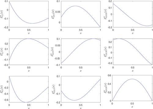
Table 1. Values of ${\left\{\genfrac{}{}{0ex}{}{n}{k}\right\}}_{\mathit{\lambda }}$.

$\mathit{k}$ $\mathit{n}$	0	1	2	3	4	5	6
0	1
1	0	1
2	0	$1-\mathit{\lambda }$	1
3	0	$1-3\mathit{\lambda }+2{\lambda }^2$	$3-3\mathit{\lambda }$	1
4	0	$1-6\mathit{\lambda }+11{\lambda }^2-6{\lambda }^3$	$7-18\mathit{\lambda }+11{\lambda }^2$	$6-6\mathit{\lambda }$	1
5	0	$1-10\mathit{\lambda }+35{\lambda }^2-50{\lambda }^3+24{\lambda }^4$	$15-70\mathit{\lambda }+105{\lambda }^2-50{\lambda }^3$	$25-60\mathit{\lambda }+35{\lambda }^2$	$10-10\mathit{\lambda }$	1
6	0	$1-15\mathit{\lambda }+85{\lambda }^2-225{\lambda }^3+274{\lambda }^4-120{\lambda }^5$	$31-225\mathit{\lambda }+595{\lambda }^2-675{\lambda }^3+274{\lambda }^4$	$90-375\mathit{\lambda }+510{\lambda }^2-225{\lambda }^3$	$65-150\mathit{\lambda }+85{\lambda }^2$	$15-15\mathit{\lambda }$	1

4. Conclusion

Let $\mathit{Y}$ be a random variable such that the moment generating function of $\mathit{Y}$ exists in a neighbourhood of the origin. In this paper, we studied by using generating functions probabilistic extensions of several special polynomials, namely the probabilistic degenerate Bernoulli polynomials associated with $\mathit{Y}$ and the probabilistic degenerate Euler polynomials associated with $\mathit{Y}$, together with the probabilistic degenerate $\mathit{r}$-Stirling numbers of the second associated with $\mathit{Y}$ and the probabilistic degenerate two variable Fubini polynomials associated with $\mathit{Y}$. In more detail, we obtained several explicit expressions for ${\beta }_{n,\lambda }^Y(\mathit{x})$ (see Theorems 1, 2, 6) and an explicit expression for each of $F_{n,\lambda }^Y(\mathit{x}|\mathit{y}),F_{n,\lambda }^Y(\mathit{y}|\mathit{r})$, and ${\mathcal{E}}_{n,\lambda }^Y(\mathit{x})$ (see Theorems 11, 12, 14). We derived three identities about probabilistic degenerate extensions of well-known identities on Bernoulli numbers and polynomials (see Theorems 3-5). Further, we obtained one identity about probabilistic degenerate extensions of well-known identity on Euler numbers and polynomials (see Theorem 16). We obtained an identity involving ${\left\{\begin{array}{c}n\\ k\end{array}\right\}}_{\mathit{Y},\mathit{\lambda }}$ and ${\beta }_{m,\lambda }^Y$ in Theorem 7 and a generalization of that identity involving ${\left\{\begin{array}{c}n+r\\ k+r\end{array}\right\}}_{r,\lambda }^Y$ and ${\beta }_{m,\lambda }^Y(\mathit{r})$ in Theorem 13. We determined explicit expressions for ${\beta }_{n,\lambda }^Y$ when $\mathit{Y}\sim \mathrm{\Gamma }(1,1)$ in Theorem 8 and $\mathit{Y}$ is the Bernoulli random variable with probability of success $\mathit{p}$ in Theorem 9. We found explicit expressions for ${\mathcal{E}}_{n,\lambda }^Y$ when $\mathit{Y}\sim \mathrm{\Gamma }(1,1)$ in Theorem 17 and $\mathit{Y}$ is the Poisson random variable with parameter $\mathit{\alpha }>0$ in Theorem 18. We deduced an explicit expression for ${\left\{\begin{array}{c}n+r\\ k+r\end{array}\right\}}_{r,\lambda }^Y$ in Theorem 10.

As one of our future projects, we would like to continue to study probabilistic versions of many special polynomials and numbers and to find their applications to physics, science and engineering as well as to mathematics

Disclosure statement

No potential conflict of interest was reported by the author(s).

Additional information

Funding

This research was funded by the National Natural Science Foundation of China (No. 12271320), Key Research and Development Program of Shaanxi (No. 2023-ZDLGY-02).

References

- Abbas M, Bouroubi S. 2005. On new identities for bell’s polynomials. Discrete Math. 293(1–3):5–10. doi: 10.1016/j.disc.2004.08.023.
- Adams CR, Morse AP. 1939. Random sampling in the evaluation of a Lebesgue integral. Bull Amer Math Soc. 45(6):442–447. doi: 10.1090/S0002-9904-1939-07003-1.
- Adell JA. 2022. Probabilistic Stirling numbers of the second kind and applications. J Theoret Probab. 35(1):636–652. doi: 10.1007/s10959-020-01050-9.
- Aydin MS, Acikgoz M, Araci S. 2022. A new construction on the degenerate Hurwitz-zeta function associated with certain applications. Proc Jangjeon Math Soc. 25(2):195–203.
- Boubellouta K, Boussayoud A, Araci S, Kerada M. 2020. Some theorems on generating functions and their applications. Adv Stud Contemp Math (Kyungshang). 30(3):307–324.
- Carlitz L. 1979. Degenerate Stirling, Bernoulli and Eulerian numbers. Utilitas Math. 15:51–88.
- Comtet L. 1974. Advanced combinatorics. The art of finite and infinite expansions. Revised and enlarged ed. Dordrecht: D. Reidel Publishing Co.
- Dolgy D, Kim W, Lee H. 2023. A note on generalized degenerate Frobenius-Euler-Genocchi polynomials. Adv Stud Contemp Math (Kyungshang). 33(2):111–121.
- Gun D, Simsek Y. 2020. Combinatorial sums involving Stirling, Fubini, Bernoulli numbers and approximate values of Catalan numbers. Adv Stud Contemp Math (Kyungshang). 30(4):503–513.
- Jang L-C. 2020. A note on degenerate type 2 multi-poly-Genocchi polynomials. Adv Stud Contemp Math (Kyungshang). 30(4):537–543.
- Kilar N, Simsek Y. 2021. Combinatorial sums involving Fubini type numbers and other special numbers and polynomials: approach trigonometric functions and p -adic integrals. Adv Stud Contemp Math (Kyungshang). 31(1):75–87.
- Kim HY, Jang LC, Kwon J. 2023. On generalized degenerate type 2 Euler polynomials. Adv Stud Contemp Math (Kyungshang). 33(1):23–31.
- Kim W, Jang L-C, Kwon J. 2022. Some properties of generalized degenerate Bernoulli polynomials and numbers. Adv Stud Contemp Math (Kyungshang). 32(4):479–486.
- Kim DS, Kim T. 2020. A note on a new type of degenerate Bernoulli numbers. Russ J Math Phys. 27(2):227–235. doi: 10.1134/S1061920820020090.
- Kim T, Kim DS. 2022a. Degenerate r-Whitney numbers and degenerate r-Dowling polynomials via boson operators. Adv Appl Math. 140(102394):21. doi: 10.1016/j.aam.2022.102394.
- Kim T, Kim DS. 2022b. Some identities on degenerate $r$-Stirling numbers via boson operators. Russ J Math Phys. 29(4):508–517. doi: 10.1134/S1061920822040094.
- Kim T, Kim DS. 2023a. Combinatorial identities involving degenerate harmonic and hyperharmonic numbers. Adv Appl Math. 148(102535):15. doi: 10.1016/j.aam.2023.102535.
- Kim T, Kim DS. 2023b. Probabilistic degenerate Bell polynomials associated with random variables. Russ J Math Phys. 30(4):528–542. doi: 10.1134/S106192082304009X.
- Kim T, Kim DS. 2023c. Some identities involving degenerate Stirling numbers associated with several degenerate polynomials and numbers. Russ J Math Phys. 30(1):62–75. doi: 10.1134/S1061920823010041.
- Kim T, Kim DS. 2024. Probabilistic Bernoulli and Euler Polynomials. Russ J Math Phys. 31(1):94–105. doi: 10.1134/S106192084010072.
- Kim T, Kim DS, Kim H. 2022. Study on r-truncated degenerate Stirling numbers of the second kind. Open Math. 20(1):1685–1695. doi: 10.1515/math-2022-0535.
- Kim T, Kim DS, Kim HK. 2023. Some identities involving Bernoulli, Euler and degenerate Bernoulli numbers and their applications. Appl Math Sci Eng. 31(1). Paper No. 2220873. doi: 10.1080/27690911.2023.2220873.
- Kim T, Kim DS, Kim HY, Kwon J. 2019. Ordinary and degenerate Euler numbers and polynomials. J Inequal Appl. 2019(1):265. doi: 10.1186/s13660-019-2221-5.
- Kim T, Kim DS, Lee H, Park J-W. 2020. A note on degenerate r-Stirling numbers. J Inequal Appl. 225(1):12. doi: 10.1186/s13660-020-02492-9.
- Lee S-H, Jang LC, Kwon J. 2023. A note on r-truncated degenerate special polynomials. Adv Stud Contemp Math (Kyungshang). 33(1):7–16.
- Leon-Garcia A. 1994. Probability and random processes for electronic engineering, Addison-Wesley series in electrical and computer engineering. New York: Addison-Wesley.
- Park J-W. 2023. On the degenerate multi-poly-genocchi polynomials and numbers. Adv Stud Contemp Math (Kyungshang). 33(2):181–186.
- Park J-W, Kim BM, Kwon J. 2021. Some identities of the degenerate Bernoulli polynomials of the second kind arising from λ-Sheffer sequences. Proc Jangjeon Math Soc. 24(3):323–342.
- Pyo S-S. 2018. Degenerate Cauchy numbers and polynomials of the fourth kind. Adv Stud Contemp Math (Kyungshang). 2018(1):127–138. doi: 10.1186/s13660-018-1626-x.
- Rim S-H, Jeong J. 2012. On the modified q-Euler numbers of higher order with weight. Adv Stud Contemp Math (Kyungshang). 22(1):93–98. doi: 10.1155/2012/948050.
- Roman S. 1984. The umbral calculus, pure and applied mathematics 111. New York: Academic Press, Inc. [Harcourt Brace Jovanovich, Publishers].
- Ross SM. 2019. Introduction to probability models. Twelfth edition ed. London: of Academic Press.
- Simsek Y. 2021. Construction of generalized Leibnitz type numbers and their properties. Adv Stud Contemp Math (Kyungshang). 31(3):311–323.
- Xu R, Kim T, Kim DS, Ma Y. Probabilistic degenerate Fubini polynomials associated with random variables. arXiv:2401.02638 [math.PR] 10.48550/arXiv.2401.02638.