Improved stiff string torque and drag prediction using a computationally efficient contact algorithm

ABSTRACT

Due to the intermittent contact with the wellbore, determining torque and drag for deviated wells is difficult. Most models have ignored drill string stiffness and assumed continual contact to simplify derivation. However, the accuracy of these ‘soft-string’ models is restricted, especially at high dogleg severities. On the other hand, most ‘stiff-string’ models rely on computationally intensive approaches or continuous contact assumptions. To mitigate these issues, a computationally efficient penalty-based wellbore contact algorithm has been developed based on vector calculation, which at most requires two dot products and three arithmetic operations to determine contact locations. This algorithm is incorporated into a 3D multibody dynamics (MBD) model, which utilizes rigid drill-string segments based on the Newton-Euler formulation, connected via axial, shear, torsional, and bending springs to capture drill string flexibility. This model performs simulations faster than real-time and has been validated using surface measurements from a completed well.

KEYWORDS:

• Drill-string torque and drag
• bond graph
• contact detection

1. Introduction

Directional drilling is an industry worth over 10 billion dollars and has seen tremendous technological advancement during the past few decades (Statistics 2021). Moreover, directional drilling has enabled the exploration of previously unreachable wells and has reduced exploration costs by enabling the drilling of multiple wells from a single rig (Ma et al. 2016; Etaje et al. 2022). During directional drilling, due to the curvature of the wellbore, the drill string will be in contact with the wellbore, which causes frictional forces to be applied to the drill string. In extended wells, these frictional forces can be significant, causing shear failure in the string, which limits the maximum reach of a well (Tikhonov et al. 2014). Therefore, during the well-planning stages, it is important to predict the expected torque and drag values to prevent unexpected issues from arising during operation. Moreover, high torque and drag can cause severe case wear, increase torsional vibrations, and reduce drilling efficiency. Considering all these factors, it is beneficial to predict frictional torque and drag and take necessary remedies to reduce it (Aadnoy et al. 2006; Mirhaj et al. 2016). Hence, several research studies have been focused on this area and have developed various prediction models with varying degrees of complexity and limitations. Yet, according to Mason and Chen (2007), despite the availability of torque and drag software models for over 20 years, the underlying mathematical model has only undergone minor improvements, and still, there is debate over the validity of the predictions.

The objective of this study is to develop a drill string contact algorithm that requires minimal computational effort compared to other geometry-based contact algorithms, which is especially important for complex, long-reach drill string simulation models. This torque and drag prediction model has been built by applying a novel penalty-based contact algorithm at each endpoint of the drill string segments that calculates penetration distance relative to a set of cylinders, that defines the geometry of the wellbore. A 3D multi-body dynamic (MBD) model of the drill string is utilized to implement this algorithm, and in this model, the drill string is discretized into rigid segments, which are attached together via axial, shear, bending, and torsional springs to include string flexibility.

One of the main advantages of the proposed ‘fast contact torque and drag’ (FCTD) model is the modelling simplicity and computational speed. This enables drilling engineers to implement this model as a design tool to analyse various drilling profiles by changing parameters and using the simulation data to select the most suitable well profile. Moreover, compared to other torque and drag prognosis models, the FCTD algorithm is intuitive to understand, which would reduce user errors. According to Çağlayan and Kağan (Çağlayan 2014), modelling complexity and incomplete understanding of limitations have caused drilling engineers to inaccurately predict expected torque and drag values in the past, causing unexpected failures. The FCTD model runs in real-time in a simulation environment that has a visualization tool that helps to reduce the likelihood of such errors during deployment and facilitates the identification of regions where the drill string is in contact with the wellbore. Additionally, the real-time simulation capabilities of the prediction model facilitate its utilization as a diagnostic tool to identify down-hole problems by comparing the surface torque measurements against the predicted values from the FCTD model.

This paper first summarizes the advantages and limitations of torque and drag models and contact algorithms in the literature. Section 3 of this paper explains the drill string model, and Section 4 presents the contact algorithm and its implementation in the FCTD model. In Section 5, a detailed description of model parameters is provided. Validation of the FCTD algorithm using a Finite element analysis (FEA) simulation and surface measurement from a completed well is presented in Section 6, along with a comparison against a similar discretized stiff string model based on nonlinear geometric contact to demonstrate the computational advantage. Finally, the conclusion section provides a summary of the model and its future applications.

2. Literature review

2.1. Current torque and drag prediction models

Existing torque and drag prediction models can be divided into two main categories: soft string and stiff string models. In soft string models, the stiffness of the drill string is neglected, and it is assumed that the drill string maintains constant contact with the wellbore. Due to these assumptions, deriving soft string models is comparatively simple, which has aided the development of many different prediction models.

Johancsik et al. (1984). developed the earliest soft string model by defining the frictional force as a product of normal force and the friction coefficient. The normal force in this model was calculated utilizing the buoyant weight of the drill string element and the two axial tension forces at the ends of the drill string. This model was then improved by Sheppard et al. (1987). by including mud pressure and converting the model into standard differential equation form. The Johansick model was further improved by Ho (1986) with the inclusion of a stiff collar section to represent the BHA. Another widely adapted model was developed by Aadnoy and Andersen (2001) by deriving analytical expressions for friction forces in the build and drop sections of the wellbore. Later, Aadnoy and Djurhuus (Aadnoy and Djurhuus 2008) further simplified this model using geometric symmetries.

However, due to the omission of the bending stiffness, these models behave more like a rope instead of a pipe, which will give erroneous results and be inconsistent with the physical characteristics under high dogleg severity (DLS) conditions. In drilling operations, the drill string can either be in contact with the lower, top, or side walls of the wellbore and in some instances, such as in catenary curves, the drill string can hang inside the well bore without making contact for long spans (Aadnoy et al. 2006). Additionally, the bending forces could also push the drill string into the wellbore at high DLS, which further increases its frictional torque and drag. Because of the above-mentioned reasons, McSpadden and Newman (2002) recommend not to use soft string models to predict torque and drag in deviated wells with DLS higher than 30°/100 ft or when modelling stiffer tubular sections such as drill collars. Additionally, they noted prediction inaccuracies when using soft string models on wells with smaller radial clearance and recommended using stiff string models because of their realistic modelling approach.

To fix the limitations of soft string models, stiff string models have been developed during the last few decades. Menand et al. (2006). developed a drill string simulation model using beam elements and a stiff string contact model called ABIS. This contact algorithm uses an iterative process that calculates contacts one after another, starting from the bit, and due to this iterative approach, the computational requirement could be high for long-deviated wells. Tikhonov et al. (2006, 2014), developed a computationally fast stiff string model that included the wellbore radial clearances and intermittent drill string contacts, but due to the projection of the drill string onto the axial and tangent axes of the hole, the formulation can be complicated.

The finite element method (FEM) is another modelling technique utilized by some researchers to build stiff string torque and drag prediction models. These approaches tend to require fine meshes with high element counts to prevent the occurrence of undesirable element aspect ratio problems that will arise due to the slenderness of the drill string. These FEA models can take a prohibitively long time time to simulate, and the contact calculation algorithms, which are usually based on nonlinear contact surfaces, further exaggerate this computational resource limitation. Askaksen et al. (2006). developed an intermittent contact stiff string model from bit to the surface using the FEA approach on the Unix platform and commented on the high computational requirement of using FEA to model the drill string because of its slenderness ratio. Furthermore, to study bottom-hole assemblies (BHAs) under static stresses, Yang et al. (2008). introduced a three-dimensional finite difference approach. Ritto et al. (2009). analysed the dynamics of the horizontal drill string using the bar model based on finite element discretization. This model also proposed a stochastic model for the friction coefficient and considered the fluid-structure interaction of the drill string. Even though stiff-string models based on FEA methodology are available in the literature, because of the reasons mentioned at the beginning of this paragraph, none of them are well-suited for parametric studies or real-time torque predictions.

Most modelling complexity when deriving a mathematical model for the stiff drill string occurs due to the intermittent contact. Thus, many stiff string models in the literature have assumed that the drill string will maintain constant contact with the lower wall of the wellbore, which would limit their accuracy under some drilling conditions but provides significantly better predictions than soft string models. The stiff string model developed by Ho (1986), which is considered the earliest stiff string torque and drag prediction model, was created based on this continuous contact assumption. This model, as well as a few other continuous contact stiff string models including (Paslay and Cernocky 1991; McSpadden and Newman 2002; Mitchell et al. 2015), have assumed the curved well sections to have constant curvature; thus, the bending stiffness of the string does not contribute to the normal force in the curved section, which would limit their applicability. Mirhaj et al. (2016). improved these models by including a non-constant curvature trajectory in which the first and second derivatives of the well paths were non-zero. Similarly, Aadnoy et al. (2010). developed a continuous contact stiff string model by including string stiffness in their previously derived models. Another stiff string model with continuous contact assumption was developed by Oydere and Gray (2020), which used cubic splines for the well profile, and the motion of the drill string was simulated by solving three non-linear coupled ordinary differential equations at each survey point. However, this model and all the other continuous contact models mentioned in this paragraph are incapable of modelling realistic contact behaviour at high dog leg severities due to the continuous contact assumption. Mitchell et al. (2015). focused on partially fixing this limitation by developing a model that restricts the drill pipe displacement to be fixed to the lower well wall only to a finite number of distinct points defined by the drill pipe tool joints. However, some well profiles, such as catenary profiles, could have large sections where the drill string is not in contact with the wall, and all models mentioned in this paragraph will produce inaccurate results in these conditions. Furthermore, most soft/stiff string models and FEA drill string models calculated contact after static equilibrium, which assumes the drill string is not moving and no net external forces are applied. Therefore, these models do not include transient effects and velocity terms in their formulation.

Drill string vibrational analysis is another research area that focuses on the complex contact of drill string and wellbore. Even though the objective of such models is to predict the vibrational characteristics of deviated drill strings, these models can be modified to predict torque and drag behaviours. Liu and Gao (2017). is a nonlinear dynamic model that uses the Pythagorean theorem to model contact between the deviated well and the drill string. Sarker et al. (2017). focus on modelling the torsional and longitudinal motions of horizontal wellbores. In (Sarker et al. 2017), contact in the horizontal wellbore sections is calculated based on the Pythagorean theorem using the simulation coordinates for each drill string segment and the contact forces on the build section of the well were modelled based on the Johancsik et al. (1984). soft string approach modified to include stick-slip friction in addition to the sliding friction. Hence, there are limitations when modelling highly deviated wells.

Considering the length of the drill string and its intricate contact behaviour, developing stiff string models is difficult or requires high computational power to simulate a drilling operation accurately. Due to this complexity, soft-string variants are the workhorse of today’s drilling industry, even though they have many modelling limitations and inaccuracies (Etaje et al. 2022). In addition to the published models in the literature, there are few commercial software options available for drilling engineers. However, the limited information available due to the assumptions in these models could result in unrealistic predictions when used in some drilling conditions. Machine learning is another novel approach recently utilized to predict torque and drag (Elzenary 2021;Shuo et al. 2021; Bai et al. 2022). However, these models still have many restrictions due to the scarcity of available modelling data, high computational requirements, and unpredictable black-box behaviour of the algorithm. Because of these reasons, the deployment of these models in industry is controversial. In summary, looking at the literature, the development of fast and accurate torque and drag prediction models for deviated wells remains an open research question, which this research work plans to addresses.

2.2. Current contact algorithms

Most contact detection algorithms used in discrete segment simulations are based on spheres due to their ease of detecting contact, which can be done by comparing the distance between centres with sphere radii. Moreover, irregular shapes in these algorithms can be modelled using a clumped group of spheres (Kodam et al. 2010). However, this approach will not be accurate for modelling the drill string due to its cylindrical geometry. Contact detection algorithms have been developed for non-spherical primitives such as ellipse (Ting 1992), ellipsoids (Lin and Ng 1995), and polyhedral (Zhou et al. 2015), which are applicable for various applications. However, there is still a lack of widely accepted contact theory geometries with edges and sharp corners, such as cylinders, which are required to model the drill string (Feng et al. 2017).

Kodam et al. (2010). proposed a cylindrical contact calculation method in which the various contact scenarios were identified, and collation for these scenarios was calculated separately. This procedure can have limited accuracy for certain modelling scenarios and requires significant calculations. Chittawadigi and Saha (2013) proposed a cylindrical contact algorithm that utilized the axisymmetric nature of the cylinders to simplify the contact tests yet requires significant calculation steps, which prevents the use of this algorithm for the long slender profile of the drill string. Feng and Owen (2004) developed a two-stage cylindrical contact algorithm based on asymmetric properties. This algorithm simplifies the 3D cylinder-cylinder intersection problem to a series of 2D circle-ellipse intersection problems. However, this approach also becomes complicated and of limited accuracy when applied to the drill applications due to the need to consider various intersection types. Even though there are contact models for cylinders available in the literature, there remains a need for an efficient, easily implemented contact algorithm suited to drill strings.

3. Drill string model

To calculate the string dynamics and to implement the contact algorithm for torque and drag prognosis, an MBD simulation model of the drill string is needed. Research work done by Rideout et al. (2013). which uses the vector bond graph technique, was selected as the foundation of the drill string simulation model used in this paper.

3.1. Bond graph (BG) methodology

Bond graphs (BG) are a multidisciplinary modelling approach that graphically represents the energy structure of a system using only a few different element types. Moreover, BG notation provides a concise description of a complex system and aids in formulating the governing system equations (Borutzky 2010).

In this methodology, energy is stored by capacitors (C) and inertias (I) as a function of state variables, which are generalized displacements (q) and momenta (p). The time derivatives of these state variables are flow (f) and effort (e), and the product of those is power. Energy dissipation occurs through the generalized resistor (R) elements, and the system’s interaction with the environment is represented via the source of effort (Se) and flow (Sf) ports. Transformers (TF) and gyrators (GY) are elements that convert energy ideally either in one physical domain or between one domain and another. A summary of commonly used BG elements is given in Table 1.

Table 1. Bond graph elements

Variables	Symbol	Constitutive law	Causality constraints
Flow		$\mathit{f}=\mathit{f}(\mathit{t})$	Fixed flow out
Effort		$\mathit{e}=\mathit{e}(\mathit{t})$	Fixed effort out
Inertia		$\mathit{f}=\frac{1}{I}\int \mathit{e}\mathit{dt}$	Preferred integral
		$\mathit{e}=\mathit{I}\frac{\mathit{df}}{\mathit{dt}}$
Capacitor		$\mathit{e}=\frac{1}{C}\int \mathit{f}\mathit{dt}$	Preferred integral
		$\mathit{f}=\mathit{C}\frac{\mathit{de}}{\mathit{dt}}$
Resistor		$\mathit{e}=\mathit{R}\mathit{f}$	None
		$\mathit{f}=\frac{1}{R}\mathit{e}$
Transformer		$\begin{array}{rl}& e_2=\mathit{n}{f}_1\\ & f_1=\mathit{n}{f}_2\end{array}$	Flow-in effort-out or Effort-in flow-out
Gyrator		$\begin{array}{rl}& e_2=\mathit{n}{f}_1\\ & f_1=\mathit{n}{f}_2\end{array}$	Effort-in effort-out or flow-in flow-out
1-junction		$\begin{array}{rl}& e_2=e_1-e_3\\ & f_1=f_2=f_3\end{array}$	One flow input
0-junction		$\begin{array}{rl}& f_2=f_1-f_3\\ & e_1=e_2=e_3\end{array}$	One flow input

In the bond graph diagram, elements are joined together using half-arrows which indicate the direction of positive power flow, and are bonded to 0-junctions or 1-junctions, which enforce Kirchoff’s loop and node power-conservation laws. Causal strokes marked on the half arrows indicate whether the effort or flow variable is the input or output from the constitutive law of the connected elements, which aids the formulation of system equations and provides intuition about the system’s behaviour. The readers can refer to Karnopp et al. (2012). for a comprehensive description of the bond graph approach.

3.2. Multibody BG drill string model description

As explained earlier, the MBD drill string model developed by Rideout et al. (2013). was selected to implement the drill string dynamics. In this model, the drill string is discretized into 3D rigid segments with six degrees of freedom. These are connected via axial, torsional, and bending springs to include flexibility, as shown in Figure 1.

Figure 1. Discetized drill string segments are connected together with axial, torsional, and bending springs (all are included simultaneously).

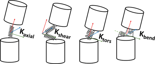
Each of these 3D BG rigid segments has been modelled based on the Euler junction structure formulation and dynamics of bodies undergoing large motions, which was represented by the following governing equations (Karnopp et al. 2012),

(1) $\mathrm{\Sigma }{}^0\mathit{F}=\frac{d}{\mathit{dt}}\left(\mathit{m}{}^0{V}_{\mathit{Gi}}\right)=m^0{\dot{V}}_{\mathit{Gi}}$(1)

(2) ${\mathrm{\Sigma }}^i\mathit{M}=\frac{d}{\mathit{dt}}\left(J^i{\omega }_i\right)=J^i{\dot{\omega }}_{\mathit{i}}{+}^i{\omega }_i\times J^i{\omega }_i$(2)

In the above equations, the left superscript 0 indicates that the vector is resolved in the inertial frame, and superscript i indicates that the vector is resolved in the body-fixed frame. To facilitate the application of gravitational force, the translational equations are expressed in the inertial reference frame. The two terms on the right-hand side of the rotational equation are the inertial term and the gyrational term.

When developing this subsystem, the velocity of the hinge point A in the body-fixed frame (${ }^1{\overrightarrow{V}}_{\mathit{Ai}}$) can be defined as (B is defined similarly)

(3) ${ }^1{\overrightarrow{V}}_{\mathit{Ai}}{=}^1{\overrightarrow{V}}_{\mathit{Gi}}{+}^1{\overrightarrow{V}}_{\mathit{Ai}/\mathit{Gi}}$(3)

(4) ${ }^1{\overrightarrow{V}}_{\mathit{Ai}/\mathit{Gi}}{=}^i{\overrightarrow{\omega }}_{\mathit{i}}{\times }^i{\overrightarrow{r}}_{\mathit{Ai}/\mathit{Gi}}{=}^1{{\tilde{r}}_{\mathit{Ai}/\mathit{Gi}}}^{\mathit{i}}{\overrightarrow{\omega }}_{\mathit{i}}$(4)

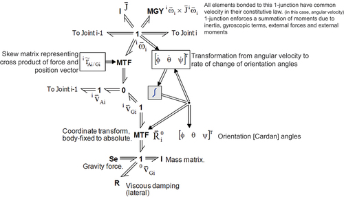
where ${ }^1{\overrightarrow{r}}_{\mathit{Ai}/\mathit{Gi}}$ is the position vector from G to A, and ${ }^1{\tilde{r}}_{\mathit{Ai}/\mathit{Gi}}$ is a skew-symmetric matrix containing the relative position vector components. Figure 2 shows a top-level vector bond graph representation of the above equations. More details about this model and its derivations can be found by referring to Rideout et al. (2013).

Figure 2. BG formulation of 3D rigid drill string MBD segment (Rideout et al. 20131984).

4. The contact algorithm

The ‘fast point in the cylinder’ is a contact algorithm developed by James (2008) to model contact of the character’s arms and legs in computer games. This algorithm uses at most two dot products, a subtract, and two multiplies to determine if a point lies within the cylindrical volume. Hence, the computational requirement is comparably lower when compared with other general-purpose or cylindrical nonlinear contact algorithms. This research work extends this algorithm to develop a fast, stiff string torque and drag prediction model based on penalty-based contact that could be easily implemented for various drilling conditions.

Implementation of the contact algorithm and development of the FCTD model can be divided into five stages.

1. Defining wellbore profile and drill string segment endpoints

2. Identifying the matching wellbore cylinder for each endpoint

3. Calculating penetration distance

4. Calculating contact force and direction

5. Applying contact force vector in the MBD model

4.1. Defining wellbore profile and drill string endpoints

This contact algorithm has been designed to compare each drill string segment’s top surface centre point (T) against the wellbore geometry to identify contact points and forces. The positions of point T have been calculated using the MBD model, and the wellbore geometry has been modelled using a set of cylinders. Each wellbore cylinder has been defined using two points (A and B) that lie on the centre of the top and bottom cylinder flat (cap) surfaces defined based on the survey depth, inclination, and azimuth. This approximation of discretizing the wellbore into a set of cylinders is necessary to implement the proposed contact algorithm and significantly improve its performance. More details about the procedure of defining the wellbore profile in the FCTD implementation can be found in Section 5.2.

4.2. Identifying the matching wellbore cylinder for each endpoint

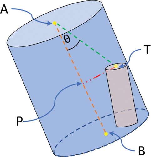
To calculate contact, the algorithm must first identify which wellbore cylinder should be considered for each drill string segment endpoint. This is accomplished by using the fact that the dot product of two vectors is equal to the product of the length of each vector multiplied by the cosine of the angle between them. This calculation will be performed at each simulation timestep, examining each wellbore cylinder one after the other using a FOR-loop until the wellbore cylinder that matches with each drill sting segment endpoint has been found.

The two vectors used for the dot product calculation have been constructed between $\overrightarrow{\mathit{AB}}$ and $\overrightarrow{\mathit{AT}}$, as shown in Figure 3. Here $\overrightarrow{\mathit{AB}}$ vector represents the centerline of the wellbore cylinder and $\overrightarrow{\mathit{AT}}$ represent the vector between the wellbore cylinder top and drill string segment center endpoint (T). The dot product (Q) between $\overrightarrow{\mathit{AB}}$ and $\overrightarrow{\mathit{AT}}$ vectors can be calculated using two methods as shown below. In Equation 5(5) $\mathit{Q}={\overrightarrow{(\mathrm{AB})}}_{\mathit{x}}{\overrightarrow{(\mathrm{AT})}}_{\mathit{x}}+{\overrightarrow{(\mathrm{AB})}}_{\mathit{y}}{\overrightarrow{(\mathrm{AT})}}_{\mathit{y}}+{\overrightarrow{(\mathrm{AB})}}_{\mathit{z}}{\overrightarrow{(\mathrm{AT})}}_{\mathit{z}}$(5) , subscript indicates the vector component in the x, y, and z directions.

Figure 3. Test cylinder and the test point used in the 3D contact algorithm.

(5) $\mathit{Q}={\overrightarrow{(\mathrm{AB})}}_{\mathit{x}}{\overrightarrow{(\mathrm{AT})}}_{\mathit{x}}+{\overrightarrow{(\mathrm{AB})}}_{\mathit{y}}{\overrightarrow{(\mathrm{AT})}}_{\mathit{y}}+{\overrightarrow{(\mathrm{AB})}}_{\mathit{z}}{\overrightarrow{(\mathrm{AT})}}_{\mathit{z}}$(5)

(6) $\mathit{Q}=|\overrightarrow{\mathrm{AB}}||\overrightarrow{\mathrm{AT}}|\mathit{cos\theta }$(6)

For the condition where the test point (T) is located at the top cap of the wellbore cylinder, the dot product between $\overrightarrow{\mathit{AB}}$ and $\overrightarrow{\mathit{AT}}$ would be zero based on the fact that the cosine of two perpendicular vectors is zero as indicated in Figure 4(a). Consequently, if the dot product between these two vectors is negative, it can be concluded that the string segment endpoint (T) is located above the selected wellbore cylinder. Moreover, if the test point is located at the bottom cap of the cylinder, then the value of the dot product will be equal to the square of the length of the selected wellbore cylinder due to the projection of $\overrightarrow{\mathit{AT}}$ onto $\overrightarrow{\mathit{AB}}$ by the cosine function as indicated in Figure 4(b).

Figure 4. When drill string endpoint is located at the top or bottom of the wellbore cylinder.

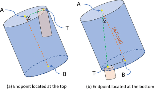
Using the above information, a verification of whether the test point lies between the top and bottom cylinder planes can be calculated by analysing the sign of the dot product (Q) and comparing it against the square of the cylinder height. This step would be iterated until the wellbore cylinder that matches with the drill string segment endpoint is calculated, and this implementation can be seen from the discussion box in Figure 7. It should be noted that the above calculation only inspects the location of the test point (T) relative to the top and bottom cylinder planes and will not determine if it is located inside or outside the cylinder. The next stage of the algorithm accomplishes this in conjunction with the penetration distance calculation. Furthermore, to handle the condition where the test point is located exactly at the top or bottom of the wellbore cylinder and also to prevent abrupt changes in contact forces, an overlap region was introduced to the wellbore cylinders, and more information about this implementation is given in Section 5.2.

4.3. Calculating penetration distance

To calculate the penetration distance, the magnitude of $\overrightarrow{\mathit{PT}}$ is needed, which is the perpendicular distance between the segment test point (T) and the axis of the wellbore segment (AT) as shown in Figure 3. This will be calculated by projecting $\overrightarrow{\mathit{AT}}$ as shown in Equation 7.

(7) $|\overrightarrow{\mathrm{PT}}|=|\overrightarrow{\mathrm{AT}}|\mathit{sin\theta }$(7)

The above equation was squared and the ${sin}^2\mathit{\theta }$ term was replaced using Equation 6 to simplify the calculation steps of the algorithm,

(8) $|\overrightarrow{\mathrm{PT}}{|}^2=|\overrightarrow{\mathrm{AT}}{|}^2\mathit{si}{n}^2\mathit{\theta }$(8)

(9) $=|\overrightarrow{\mathrm{AT}}{|}^2(1-\mathit{co}{s}^2\mathit{\theta })$(9)

(10) $=|\overrightarrow{\mathrm{AT}}{|}^2\left(1-\frac{Q^2}{|\overrightarrow{\mathrm{AB}}{|}^2|\overrightarrow{\mathrm{AT}}{|}^2}\right)$(10)

During each simulation time step, the penetration distance (D) of the endpoint into the wellbore cylinder will be calculated by deducting the difference between the wellbore radius ($r_{\mathit{bh}}$) and the drill-string radius ($r_{\mathit{ds}}$) from the calculated magnitude of $\overrightarrow{\mathit{PT}}$ using Equation 10. The magnitude of the contact force ($F_n$) for illustrative purposes will be obtained by multiplying the penetration distance (D) with the contact stiffness (K) as shown in Equation 12. This equation is based on simple linear contact stiffness law; however, the modeller can implement more sophisticated non-linear relations if desired.

(11) $\mathit{D}=(r_{\mathit{bh}}-r_{\mathit{ds}})-|\overrightarrow{\mathrm{PT}}|$(11)

(12) $F_n=\mathit{K}\ast \mathit{D}$(12)

4.4. Calculating force direction

The contact algorithm developed by James (2008) did not include a method to calculate the direction of the contact force. The current application requires a method to calculate the vector perpendicular to the wellbore axis and the drill string segment endpoint, thus representing the direction of the normal contact force.

As the first step of obtaining the unit vector for the contact force, an arbitrary point (S) on the cylinder axis, as shown in Figure 5, has been defined using the Equation 14(14) $\mathit{\lambda }=\frac{\left(\overrightarrow{\mathrm{A}}-\overrightarrow{\mathrm{B}}\right).\left(\overrightarrow{\mathrm{A}}-\overrightarrow{\mathrm{T}}\right)}{\left(\overrightarrow{\mathrm{A}}-\overrightarrow{\mathrm{B}}\right).\left(\overrightarrow{\mathrm{A}}-\overrightarrow{\mathrm{B}}\right)}$(14) . In this equation the value of $\mathit{\lambda }$ defines all possible points located on the $\overrightarrow{\mathit{AB}}$ vector,

Figure 5. Arbitrary vector going through test point (T) and point in cylinder axis (S).

(13) $\mathit{S}=\overrightarrow{\mathrm{A}}+\mathit{\lambda }\left(\overrightarrow{\mathrm{A}}-\overrightarrow{\mathrm{B}}\right)$(13)

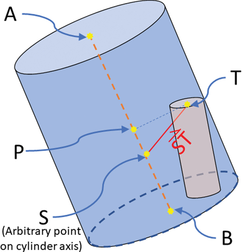
To represent the force direction, $\overrightarrow{\mathit{ST}}$ must be perpendicular to $\overrightarrow{\mathit{AB}}$ and the value of $\mathit{\lambda }$ that satisfies this condition has been calculated based the fact that the dot product of two perpendicular vectors is equal to zero.

(14) $\mathit{\lambda }=\frac{\left(\overrightarrow{\mathrm{A}}-\overrightarrow{\mathrm{B}}\right).\left(\overrightarrow{\mathrm{A}}-\overrightarrow{\mathrm{T}}\right)}{\left(\overrightarrow{\mathrm{A}}-\overrightarrow{\mathrm{B}}\right).\left(\overrightarrow{\mathrm{A}}-\overrightarrow{\mathrm{B}}\right)}$(14)

After calculating $\mathit{\lambda }$, the value has been substituted in Equation 14(14) $\mathit{\lambda }=\frac{\left(\overrightarrow{\mathrm{A}}-\overrightarrow{\mathrm{B}}\right).\left(\overrightarrow{\mathrm{A}}-\overrightarrow{\mathrm{T}}\right)}{\left(\overrightarrow{\mathrm{A}}-\overrightarrow{\mathrm{B}}\right).\left(\overrightarrow{\mathrm{A}}-\overrightarrow{\mathrm{B}}\right)}$(14) and using this point, $\overrightarrow{\mathit{ST}}$ has been calculated. For the calculated $\mathit{\lambda }$ value, the point (S) would be equal to previously defined (P) and $\overrightarrow{\mathit{ST}}$ would be equal $\overrightarrow{\mathit{PT}}$ which is the force direction.

4.5. Calculating frictional forces

The frictional drag force $(F_{\mathit{fric}})$ on the drill string segment has been calculated by multiplying the contact force ($F_n$) with the frictional coefficient, and the direction of the frictional drag force was assumed to be parallel to the direction of the drill string segment cylinder axis. The frictional torque $(T_{\mathit{fric}})$ has been calculated by multiplying the frictional force with the drill string radius, and the direction was assumed to be perpendicular to the contact force and frictional drag. The equations for both frictional forces are given below, and the summation of these forces of all drill string segments will provide the total frictional torque and drag value of the off-bottom drill string.

(15) $F_{\mathit{fric}}=\mathit{sign}\left(\mathit{V}\right)\left|\mathit{\mu }{F}_n\right|$(15)

(16) $T_{\mathit{fric}}=r_{\mathit{ds}}{F}_{\mathit{fric}}$(16)

This simplistic frictional approach may be sufficient for preliminary static design studies. However, if this model is utilized to analyse complex drill string dynamics, a frictional model with static and dynamic frictional coefficients must be implemented, for example, Karnopp (1985), which efficiently overcomes simulation challenges due to nonlinearities of the frictional coefficient. In the future, the authors of this paper plan to expand this research work by including a similar frictional model to analyse the drill string whirling vibration in highly deviated wells.

4.6. Implementing the contact and frictional force in the MBD model

The contact calculation algorithm is applied at the drill string endpoint between two 3D rigid drill string MBD segments, as shown in Figure 6. In this figure, double lines represent vector signals or vector power bonds, which containing the x, y, and z components.

Figure 6. BG model of the drill string with the contact algorithm.

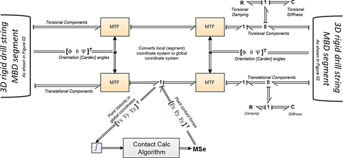
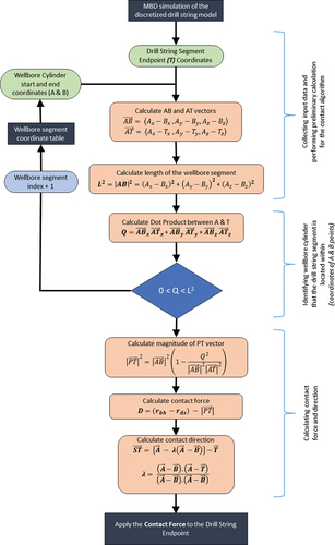
As shown in Figure 6, The x,y, and z velocity signal components from the 1-Junction will be fed into the integrator block to calculate the drill string segment endpoint position in the global coordinate system. This position data, along with the wellbore profile, contact stiffness, and radius, has been provided to the ‘contact calculation code’ block, which encapsulates the FCTD algorithm. A flowchart of the calculation methodology is given in Figure 7.

Figure 7. Summary of contact calculation algorithm.

5. Model parameters

To maximize the utility of the model in both academic and industry implementations, the model uses only parameters that are either measurable or estimable by drilling engineers. Moreover, the use of clearly defined modelling parameters also reduces the likelihood of user errors, further increasing the accuracy and the dependability of the simulation model. Hence, the focus of this section is to provide detailed descriptions of the model parameters and summarize their influence on the simulation.

5.1. Segment stiffness calculations

The drill string and collar sections have been defined only by using the length, inner diameter, outer diameter, and material properties. In addition to these parameters, the number of segments could also be modified if the accuracy or the computational efficiency of this model needed to be further increased. After defining these parameters, the model calculates axial, bending, shear, and torsional spring stiffness values, which are attached between adjacent rigid drill string segments (Karnopp et al. 2012).

(17) $K_{\mathit{tors}}=\frac{\mathit{GJ}}{\mathrm{\Delta z}}$(17)

(18) $K_{\mathit{bend}}=\frac{\mathit{EI}}{\mathrm{\Delta z}}$(18)

(19) $K_{\mathit{shear}}=\mathit{\kappa }\frac{\mathit{AG}}{\mathrm{\Delta z}}$(19)

In the above equations, $\mathrm{\Delta z}$ is the segment length, A is cross-sectional area, I is area moment, J is polar moment of area, E and G are elastic modulus and shear modulus respectively. The shear parameter was calculated based on the Timoshenko beam theory, and $\mathit{\kappa }$ is the Timoshenko shear coefficient, which considers the non-uniform shear behaviour of the cross-section geometry. For hollow cylindrical cross-sections, $\mathit{\kappa }$ can be calculated using the below equation published by Hutchinson (2001) and, in this equation, a and b represent the inner and outer radii.

(20) $\mathit{\kappa }=\frac{6(a^2+b^2{)}^2(1+\mathit{\upsilon })}{7a^4+34a^2{b}^2+7b^4+\mathit{\upsilon }(12a^4+48a^2{b}^2+12b^4)}+{\upsilon }^2(4a^4+16a^2{b}^2+4b^4)$(20)

Additionally, these parameters can be estimated using FEA approaches for complex drill string geometries, which include tools joints and other BHA equipment similar to the research work done by Galagedarage Don and Rideout (2022).

5.2. Wellbore profile

As previously mentioned, the well profile has been defined using a set of Cartesian coordinates for each wellbore cylinder, and these could be calculated using survey depth, inclination, and azimuth, which are readily available in any drilling operation based on the average angle method using the equation given below.

(21) $L_n=\sum _{\mathit{n}=1}^n{D}_{\mathit{Mi}}(sin\frac{{\alpha }_i+{\alpha }_{\mathit{i}-1}}{2})(cos\frac{{ϵ}_i+{ϵ}_{\mathit{i}-1}}{2})$(21)

(22) $M_n=\sum _{\mathit{n}=1}^n{D}_{\mathit{Mi}}(sin\frac{{\alpha }_i+{\alpha }_{\mathit{i}-1}}{2})(sin\frac{{ϵ}_i+{ϵ}_{\mathit{i}-1}}{2})$(22)

(23) $D_n=\sum _{\mathit{n}=1}^n{D}_{\mathit{Mi}}(cos\frac{{\alpha }_i+{\alpha }_{\mathit{i}-1}}{2})$(23)

In the above equations, $\mathit{\alpha }$ is equal to inclination, $\mathit{\epsilon }$ is azimuth and $D_{\mathit{Mi}}$ represents incremental changes in true vertical depth. By resolving these equations, north ($L_n$), east ($M_n$), and total vertical depth $(D_n$) could be calculated, which would correspond to the Cartesian coordinates of the well bore profile of the simulation model. A sample calculation for a well profile is given in Table 2 and North ($L_n$), East ($M_n$), and TVD $(D_n$) in this table are equal to the x, y, and z coordinates of the wellbore cylinder segments.

Table 2. Sample well profile calculation in cartesian coordinates.

SurveyDepth (m)	Incli. (α) (deg)	Azim. ($\mathit{\epsilon }$) (deg)	$\mathrm{\Delta }$TVD $(D_{\mathit{Mi}})$ (m)	$\mathrm{\Delta }$North $(\mathrm{\Delta }{L}_n)$ (m)	$\mathrm{\Delta }$East $(\mathrm{\Delta }{M}_n)$ (m)	TVD (Dn) (m)	North (Ln) (m)	East (Mn) (m)
0	0	0	0.00	0.00	0.00	0.00	0.00	0.00
1000	0	0	1,000.00	0.00	0.00	1,000.00	0.00	0.00
1050	5	0	49.95	2.18	0.00	1,049.95	2.18	0.00
1100	10	0	49.57	6.53	0.00	1,099.53	8.71	0.00
1150	15	0	48.82	10.82	0.00	1,148.34	19.53	0.00
1200	20	0	47.69	15.04	0.00	1,196.03	34.56	0.00
1250	25	0	46.20	19.13	0.00	1,242.23	53.70	0.00
1300	30	0	44.36	23.09	0.00	1,286.58	76.79	0.00
1350	35	0	42.18	26.86	0.00	1,328.76	103.65	0.00
1400	40	0	39.68	30.44	0.00	1,368.44	134.09	0.00
1450	45	0	36.88	33.78	0.00	1,405.31	167.87	0.00
1500	45	5	35.37	35.32	1.54	1,440.68	203.19	1.54
1550	45	10	35.37	35.05	4.61	1,476.05	238.24	6.16
1600	45	15	35.37	34.52	7.65	1,511.42	272.76	13.81
1650	45	20	35.37	33.72	10.63	1,546.79	306.48	24.44
1700	45	25	35.37	32.66	13.53	1,582.16	339.14	37.97
1750	45	30	35.37	31.36	16.33	1,617.53	370.50	54.30
1800	45	30	35.37	30.62	17.68	1,652.90	401.12	71.97

When defining the wellbore profile for the simulation, an overlap between cylinders has been applied to prevent gaps in the wellbore profile due to the angle difference of cylinders, as shown in Figure 8. The calculation of the overlap is done by extending the length of the cylinder by a fixed amount along its axis by modifying the wellbore cylinder segment end-point. The contact calculation algorithm is also modified to perform penetration distance (contact) calculations for both wellbore cylinder segments during the overlap region and will be combined using Equation 24(24) $|\overrightarrow{\mathrm{PT}}{|}_{\mathit{avg}}=\left(\frac{{\mathit{L}}_{\mathit{ws}}-\sqrt{\mathit{Q}}}{L_{\mathit{ol}}}\right)|\overrightarrow{\mathrm{PT}}{|}_{\mathit{now}}+\left(1-\frac{{\mathit{L}}_{\mathit{ws}}-\sqrt{\mathit{Q}}}{L_{\mathit{ol}}}\right)|\overrightarrow{\mathrm{PT}}{|}_{\mathit{next}}$(24) to prevent errors and abrupt changes.

Figure 8. The gap between wellbore cylinders and overlap.

(24) $|\overrightarrow{\mathrm{PT}}{|}_{\mathit{avg}}=\left(\frac{{\mathit{L}}_{\mathit{ws}}-\sqrt{\mathit{Q}}}{L_{\mathit{ol}}}\right)|\overrightarrow{\mathrm{PT}}{|}_{\mathit{now}}+\left(1-\frac{{\mathit{L}}_{\mathit{ws}}-\sqrt{\mathit{Q}}}{L_{\mathit{ol}}}\right)|\overrightarrow{\mathrm{PT}}{|}_{\mathit{next}}$(24)

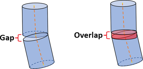
In the above equation, ($L_{\mathit{ws}}$) is the length of the wellbore segment, and ($L_{\mathit{ol}}$) is the length of the overlap, which must be defined by the user. This equation will only be valid for the overlap region and during this region, the value of $|\overrightarrow{\mathrm{PT}}|$ in the FCTD algorithm will be replaced by $|\overrightarrow{\mathrm{PT}}{|}_{\mathit{avg}}$.

5.3. Rock stiffness parameters

In this model, contact forces are calculated by multiplying the calculated penetration distance by a stiffness based on the modulus of elasticity for the formation. This parameter can be obtained either by using a rock compression test or based on the data available in the literature. Even though this parameter is required for the simulation, minor inaccuracies in this parameter would not affect the torque and drag prediction unless set to an unrealistically low value. Moreover, for typical drilling operations, it is reasonable to assume that the value of the contact stiffness is very high and assume no surface deformation in the wellbore walls or on the drill string due to contact.

5.4. Viscosity and buoyant weight of drilling mud

Due to the difference in density between the drilling mud and the drill pipe, there will be a buoyant force acting on the drill string, which will reduce the contact force. Since torque and drag measurement in the FCTD model is calculated based on the normal contact force, the inclusion of the buoyancy effect of drilling mud is essential and was included by multiplying the density of the drill pipe material with the Buoyancy-Factor (BF), which is calculated using Equation 25.

To compensate for the loss of weight due to the immersion of the drilling pipe in mud, the density of the drill pipe material was modified using the BF, which is calculated using the standard Equation 25.

(25) $\mathit{BF}=1-\frac{\mathit{densit}{\mathit{y}}_{\mathit{mud}}}{\mathit{densit}{y}_{\mathit{steel}}}$(25)

The viscosity of the drilling mud is another parameter that influences the torque and drag predictions. To represent the damping effect of drilling mud, rotational and axial dampers have been introduced using R-elements into each drill string segment, as shown in Figure 6. The influence of fluid drag from drilling mud can also depend on the fluid flow rate (Mahjoub et al. 2023), and geometries/perforation (Cayeux et al. 2022) of the drilling pipes. Additionally, research work published by Liu et al. (2021). provides a comprehensive approach to include the stabilizer effect and fluid loadings on the drill string. However, for modelling simplicity and efficiency, these effects have not been considered in this research work.

5.5. Friction factor

The friction factor is one of the critical parameters and is considered the most challenging to obtain (Mason and Chen 2007). If the simulation model considers all effects that contribute to surface torque measurements, such as micro-tortuosity, viscous damping of drilling mud, and differential sticking of the pipes, then the frictional coefficient would only depend on mechanical friction. However, in most torque and drag models, these effects are not modelled separately but lumped with frictional forces. Therefore, the friction factor not only represents the true mechanical friction but also includes a multitude of other downhole effects. This is a modelling limitation and can result in inaccuracies in the torque predictions. Yet, many researchers have used this simplification to reduce modelling complexity.

Even though the FCTD model includes the effect of mud dampening, it does not include the effects of micro-tortuosity and differential striking when calculating the torque and drag predictions. Hence, the effects of these have been included with frictional torque and drag when validating against surface measurements. Moreover, because of formation types, mud lubricity, and the effects of stabilizers, providing a frictional coefficient from a datasheet or using an equation is difficult. Therefore, the best approach to select the frictional factor is by utilizing off-bottom surface torque data from a similar well or using the off-bottom torque measurements of the initial few metres of the drilled well. Using the data from the initial section is more suitable because it would include frictional components of the surface equipment such as Kelly bushing and top drive, and this approach will be used in the FCTD model validation study in Section 6.2. Moreover, as indicated in Section 4.5, this research work only considers a simple Coulomb friction model and, if needed, can be expanded by including static and dynamic frictional coefficients and stiction conditions.

5.6. Drill string and wellbore segment count

One of the key parameters affecting the simulation accuracy and speed is the drill string segment count. If the segment count has been set to a low value when compared with the total length of the well, then the discretized drill string model would not accurately capture the bending behaviour. On the contrary, increasing the segment count to an unnecessarily high value is also not the best modelling approach due to the exponential increase in computational demand. Therefore, to obtain the most optimal model, it is advisable to perform an analysis where the segment count would be incrementally increased until no changes in the predictions have been observed, and this approach has been followed when implementing the FCTD model.

6. Validation

The torque and drag model was validated quantitatively based on two approaches. First, the contact locations and forces were validated using an explicit FEA model of a scaled-down curved well section. The second validation was done by comparing off-bottom torque measurements of a completed well using the data provided by a directional services company.

6.1. Quantitative validation of contact points and force

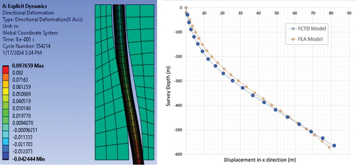
As the first stage of quantitative validation of the contact algorithm, an explicit FEA analysis was developed to analyse the accuracy of the predicted contact points and forces. Due to computational limitations and the high slenderness ratio of the drill string, modelling a complete well profile will lead to many inaccuracies and obstacles. Therefore, a scaled-down model was created in ANSYS® explicit dynamic modelling environment and a similar model was developed using the FCTD algorithm for the comparison.

As the first step of this analysis, the CAD model was developed. The curvature of the wellbore and the scale were selected using an iterative process to ensure that the drill pipe would not be crushed and that the dimensions of the ramps/pipe would not require a high element count in the FEA analysis. Due to large deformations of the drill pipe, this FEA analysis was carried out using non-linear explicit solvers, and the contact was modelled using ANSYS® penalty-based contact methods. As the boundary conditions, the wellbore CAD model was fixed to the ground, and the drill pipe was lowered into the hole by applying a constant velocity while restricting the motion in the other two directions. Automatic mass scaling was deactivated for this analysis, and the mesh was generated using quadratic elements. The average element size was selected to be 5 cm for the ramps, and the mesh sizing of the pipe was modified to be 2.5 cm to ensure at least three rows of elements along the thickness of the wall.

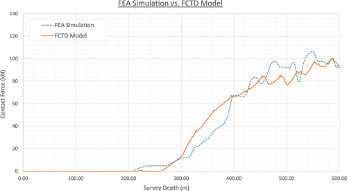
A 30-rigid segment FCTD MBD model with similar dimensions was created and lowered into the well profile to compare the results against the FEA prediction. The contact forces from both analyses are graphed in Figure 9. These results show a good correlation between the FEA model and the FCTD model. However, the results have minor differences due to the differences between meshed-based vs. rigid-segment modelling approaches used in each simulation. Yet considering the overall amplitude of the contact forces and the shape of the graph, it is accurate to assume a good correlation between the simulation results.

Figure 9. Comparision of contact force between FEA and FCTD models.

Moreover, as shown in Figure 10, both simulations predicted similar displacements in the horizontal direction and also concluded that contact points at similar locations.

Figure 10. Comparision of horizontal displacement between FEA and FCTD models.

6.2. Quantitative validation of torque and drag predictions

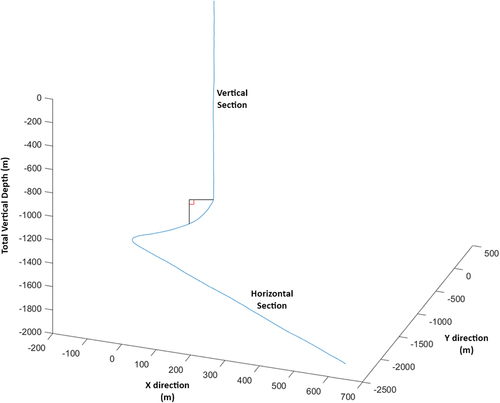
The next stage of quantitative validation was conducted using drilling measurements obtained from a completed well to validate the torque and drag predictions generated by the FCTD model. The data for this validation was taken from a well over 4300 m long with multiple curved sections with over 15° per metre dog leg severity as shown in Figure 11. In this profile, the first 1700 m are vertical. This profile has two build section between 1750 m–2450 m and the final section of this well from 2450 m–4300 m is horizontal.

Figure 11. Deviated well profile used for validation.

The drill string in this simulation model was simplified into only drill pipe and drill collar segments. All other components in the drill string, such as the bit, mud motor, reamers, and BHA measuring tool, were either omitted or represented using drill collar segments. The segment count for the simulation model was selected as 40 drill pipe segments and 20 drill collar segments after performing an analysis as explained in Section 5.6. Since the first section of the well is vertical, the first segment of the drill string was modelled as a single segment, and the axial stiffness was set accordingly. The rest of the drill pipe section was 1500 m long with an inner diameter of 60 mm and an outer diameter of 102 mm. Similarly, the drill collar section was 200 m long with segment inner and outer diameters of 65 mm and 158 mm, respectively. The frictional coefficient was selected to be 0.125 using the off-bottom torque measurement of the initial section of the well. A torque offset was also included in the model to account for all the friction components in the drilling rig, including the top drive, rotary table, and kelly bushing.

In the dataset, off-bottom torque measurements were only available up to the end of the build section. Therefore, the validation will be carried out utill 2450 m, which includes both build sections of the completed well. The results of this validation process are graphed in Figure 12, and from these results, a good correlation between the measurement data and simulation predictions was observed, validating the accuracy of the prediction model. The Measured torque plot was drawn using off-bottom torque measurements taken at a few points along the build section using surface measurement. Hence, this plot assumes linear changes in frictional torque between measurement points. This will lead to some discrepancies between the FCTD simulation and the measurement, as seen in this comparison.

Figure 12. Off-bottom torque comparison between measured vs. simulated.

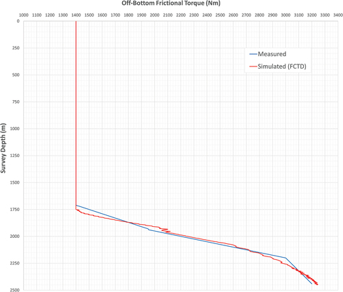
The above field data does not allow high-resolution validation of the FCTD contact algorithm at each section. However, the overall agreement of the off-bottom torque measurement from field data is a good indication that the derived FCTD model performs torque prognosis correctly since the overall torque measurement in the FCTD model is calculated by aggregating the torque measurements at each segment. Therefore, the accuracy of overall off-bottom torque values validates the accuracy of torque predictions at each segment.

6.3. Computational performance

The contact algorithm adopted in this torque and drag model is computationally less demanding when compared to other geometry-based contact approaches because it was developed specifically to model drill string contact and utilizes a streamlined algorithmic approach. To quantify the computational efficiency, a commercially available geometry-based contact algorithm was implemented in a similar discretized rigid segment MBD drill string model. For this implementation, the MSC Adams® software package was selected because of its wide industrial use and in-built efficient geometry-based contact algorithm. In addition to quantifying the computational efficiency of this research work, this analysis provides insight into modelling challenges that could arise due to the slenderness ratio of the drill pipe when using geometry-based contact algorithms for predicting drill string torque and drag behaviour.

The contact algorithm used in the MSC Adams® software package is known as RAPID (Robust and Accurate Polygon Interface Detention) and is based on the Hertzian contact theory. This algorithm draws a fine mesh over the CAD geometries and divides it into a large number of polygons. Next, the RAPID algorithm pre-computes tight-fitting oriented bounding box trees (OBBTrees), and during the simulation, overlap between trees is checked to predict the contact (Gottschalk et al. 1996). Using polygons instead of exact boundary representation would be less accurate but has the advantage of being more efficient, fast, and robust (Giesbers 2012).

Due to limitations in the modelling approaches and software packages, replicating the drill string simulation model used in the previous validation stage in MSC Adams® was infeasible. The first limitation was that the maximum size of the CAD model was 500 m. Therefore, the drill string model had to be scaled down. For modelling simplicity, it was scaled down by 1000:1, resulting in 1 m of length in the well profile, equating to 1 mm in the CAD model. Changing the metres into millimetres simplified the calculation of material properties such as density and Young’s modulus. Additionally, this scaled model followed geometric, kinematic, and dynamic similitude rules enabling accurate interpolation of scaled model results to the actual well (Szücs 2012).

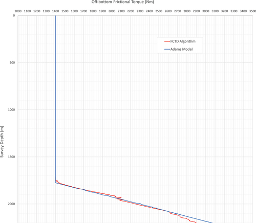
The second limitation was due to the instability of the MSC ADAMS® contact algorithm and the solver. Because of these instabilities and long simulation times, predicting torque and drag values of the complete well profile was not feasible. Therefore, as a compromise, the simulation was carried out until the end of the first build section, equating to simulation data from 0 m–2250 m of survey depth. To increase the stability, the simulation was carried out using the relative error percentage of the solver set to 0.01 and a step size of 1.5 × 10⁻⁵, which is higher than the previous simulation. The segment count also had to be increased to 120 drill pipe segments and 50 drill collar segments to match the observed torque measurements.

Simulation results and comparison against the FCTD model are given in Figure 13. A good correlation between both models can be identified from these results, which will attest to the accuracy of implementing both contact algorithms in the drill string simulation model. The MSC Adams® simulation took approximately 34 hours, compared with approximately 4 hours for the 20Sim model. These results indicate that the FCTD model was computationally more efficient and stable when compared with the ADAMS® geometry-based contact algorithm. Moreover, the FCTD model performs torque and drag analysis faster than real-time, enabling it to be utilized in many control and vibrational prediction applications, as explained previously.

Figure 13. Comparision of torque predictions between FCTD andMSC Adams® contact alogirthms.

The difference in simulation time can be attributed either to the difference in the contact detection algorithms or to the difference between modelling approaches. It should also be noted that some of the modelling differences, including the solver setting and the number of rigid segments, were due to the instabilities of the geometry-based contact algorithm. However, since the objective of this analysis is to quantify the efficiency of the proposed FCTD contact algorithm against a commercially available geometry-based contact algorithm, an approach to isolate the modelling difference from the contact algorithms has to be considered at this stage. This was achieved by measuring the time taken to simulate 150 m of the vertical tripping into the wellbore with no contact algorithms in both simulation approaches. Both models had a similar number of rigid drill string segments and similar solver settings. It took around 12 seconds for the MSC Adams® model and around 4 seconds for the FCTD/BG model to run in 20Sim. Hence, this shows that there is a computational advantage with the FCTD model when detecting contact between the drill string and the wellbore, since the FCTD algorithm is able to generate faster predictions when contact is present, beyond the advantages of the simulation environment.

7. Conclusion

An algorithm was presented to represent a petroleum exploration wellbore, or indeed any shaft enclosure, as a series of connected cylinders with overlap. A fast-point-in-cylinder algorithm was enhanced and implemented to predict the location of, and forces resulting from, contact between the drill pipes and wellbore. A vector algebra method was then developed to determine contact force directions. Finally, the contact force magnitude and frictional force/torque were computed. Validation was done using FEA simulation and surface measurement from a completed well. The torque predictions by the FCTD model were within 10% of the measured data. This difference in torque can be due to the limited availability of measured off-bottom torque data and due to modelling simplifications, which will be addressed in future work.

FCTD model performs simulations faster than real-time and has been shown to be more efficient than geometry-based nonlinear contact approaches when modelling the drill string. This prognosis model would be beneficial during the well planning stages to prevent shear failure due to high torque and drag, which reduce the maximum reach of the well. Excessive frictional forces would cause severe case wear, increase torsional vibrations, and reduce drilling efficiency. Hence, the model could also be utilized to improve the efficiency of the drilling operation. Additionally, the algorithm’s capability of performing simulations faster than real-time speeds could also be utilized as a diagnostic tool to recognize potential issues such as stuck pipes and differential sticking while drilling.

Most solutions available in the literature solve the contact determination problem under static equilibrium and do not include transient effects or velocity terms in their formulations. Due to this limitation, these models can not be utilized to accurately predict the dynamics of the drill string, unlike the FCTD model, which calculates contact points and forces to maintain the deformed drill string using a dynamic solver. In the future, the FCTD model will also be utilized in drill string vibrational analysis for deviated wells along with a nonlinear friction/stiction model. This would enable the development of new vibration reduction methods and control algorithms. Furthermore, the authors of this paper plan to implement this algorithm into a stand-alone drilling software that would enable easy adoption of this model by the drilling industry and enable diagnostic and optimization of drilling operations.

Disclosure statement

No potential conflict of interest was reported by the author(s).

Additional information

Funding

We acknowledge the support of the Natural Science and Engineering Research Council of Canada (NSERC). [Funding reference number 03887-2018].

References

- Aadnøy BS, Andersen K. 2001. Design of oil wells using analytical friction models. J Pet Sci Eng. 32(1):53–71. doi: 10.1016/S0920-4105(01)00147-4.
- Aadnoy BS, Djurhuus J. 2008. Theory and application of a new generalized model for torque and drag, In: IADC/SPE Asia Pacific Drilling Technology Conference and Exhibition. OnePetro.
- Aadnoy BS, Fazaelizadeh M, Hareland G. 2010. A 3d analytical model for wellbore friction. J Can Pet Technol. 49(10):25–36. doi: 10.2118/141515-PA.
- Aadnoy BS, Toff V, and Djurhuus J. 2006. Construction of ultralong wells using a catenary well profile, In: IADC/SPE Drilling Conference. OnePetro.
- Aslaksen H, Annand M, Duncan R, Fjaere A, Paez L, Tran U. 2006. Integrated FEA modeling offers system approach to drillstring optimization. In: IADC/SPE Drilling Conference. OnePetro.
- Bai K, Fan H, Zhang H, Zhou F, Tao X. 2022. Real time torque and drag analysis by combining of physical model and machine learning method. In: SPE/AAPG/SEG Unconventional Resources Technology Conference. OnePetro.
- Borutzky W. 2010. Analysis of causal bond graph models. In: Bond graph methodology: development and analysis of multidisciplinary dynamic system models. London: Springer London; p. 223–303. doi: 10.1007/978-1-84882-882-76.
- Çağlayan BK. 2014. Torque and drag applications for deviated and horizontal wells: a case study [ master’s thesis]. Middle East Technical University.
- Cayeux E, Stokka S, Dvergsnes E, Thorogood J. 2022. Buoyancy force on a plain or perforated portion of a pipe. Spe J. 27(1):17–38. doi: 10.2118/204025-PA.
- Chittawadigi RG and Saha SK. 2013. An analytical method to detect collision between cylinders using dual number algebra. In: 2013 IEEE/RSJ International Conference on Intelligent Robots and Systems, Tokyo, Japan. IEEE. p. 5353–5358.
- Elzenary MN. 2021. Real-time solution for down hole torque estimation and drilling optimization in high deviated wells using artificial intelligence. In: SPE Symposium: Artificial Intelligence-Towards a Resilient and Efficient Energy Industry. OnePetro.
- Etaje D, Shor R, Lashkari R. 2022. Torque and drag calculations in multilateral wells. In: SPE Nigeria Annual International Conference and Exhibition. OnePetro.
- Feng Y, Han K, Owen D. 2017. A generic contact detection framework for cylindrical particles in discrete element modelling. Comput Methods Appl Mech Eng. 315:632–651. doi: 10.1016/j.cma.2016.11.001.
- Feng Y, Owen D. 2004. A 2d polygon/polygon contact model: algorithmic aspects. Eng Comput. 21(2/3/4):265–277. doi: 10.1108/02644400410519785.
- Galagedarage Don M, Rideout G. 2022. An experimentally-verified approach for enhancing fluid drag force simulation in vertical oilwell drill strings. Math Comput Model Dyn Syst. 28(1):197–228. doi: 10.1080/13873954.2022.2143531.
- Giesbers J. 2012. Contact mechanics in msc adams-a technical evaluation of the contact models in multibody dynamics software msc adams [ B.S. thesis]. University of Twente.
- Gottschalk S, Lin MC, Manocha D. 1996. OBBTree: a hierarchical structure for rapid interference detection, In: Proceedings of the 23rd Annual Conference On Computer Graphics and Interactive Techniques, New Orleans, Louisiana, USA. p. 171–180.
- Ho HS. 1986. General formulation of drillstring under large deformation and its use in BHA analysis. In: SPE Annual Technical Conference and Exhibition. OnePetro.
- Hutchinson J. 2001. Shear coefficients for timoshenko beam theory. J Appl Mech. 68(1):87–92. doi: 10.1115/1.1349417.
- James G. 2008. Fast point-in-cylinder test. https://www.flipcode.com/archives/Fast_Point-In-Cylinder_Test.shtml.
- Johancsik C, Friesen D, Dawson R. 1984. Torque and drag in directional wells-prediction and measurement. J Pet Technol. 36(6):987–992. doi: 10.2118/11380-PA.
- Karnopp D. 1985. Computer simulation of stick-slip friction in mechanical dynamic systems. J Dyn Syst Meas Control. 107(1):100–103. doi: 10.1115/1.3140698.
- Karnopp DC, Margolis DL, Rosenberg RC. 2012. System dynamics: modeling, simulation, and control of mechatronic systems. 5th ed. Hoboken, New Jersey: John Wiley & Sons.
- Kodam M, Bharadwaj R, Curtis J, Hancock B, Wassgren C. 2010. Cylindrical object contact detection for use in discrete element method simulations. part i–contact detection algorithms. Chem Eng Sci. 65(22):5852–5862. doi: 10.1016/j.ces.2010.08.006.
- Lin X, Ng TT. 1995. Contact detection algorithms for three-dimensional ellipsoids in discrete element modelling. Num Anal Meth Geomechanics. 19(9):653–659. doi: 10.1002/nag.1610190905.
- Liu Y, Gao D. 2017. A nonlinear dynamic model for characterizing downhole motions of drill-string in a deviated well. J Nat Gas Sci Eng. 38:466–474. doi: 10.1016/j.jngse.2017.01.006.
- Liu Y, Gao D, Agarwal V, Zheng X, Balachandran B, Gan J. 2021. Drillstring oscillations: the influence of fluid loading and stabilizer effects. Shock Vib. 2021:1–10. doi: 10.1155/2021/8888837.
- Ma T, Chen P, Zhao J. 2016. Overview on vertical and directional drilling technologies for the exploration and exploitation of deep petroleum resources. Geomech Geophys Geo-Energy Geo-Resour. 2(4):365–395. doi: 10.1007/s40948-016-0038-y.
- Mahjoub M, Dao NH, Summersgill M, Menand S. 2023. Fluid circulation effects on torque and drag results, modeling, and validation. SPE Drill Complet. 38(4):594–605. doi: 10.2118/212558-PA.
- Mason CJ, Chen DCK. 2007. Step changes needed to modernize T&D software. In: SPE/IADC Drilling Conference. OnePetro.
- McSpadden A, Newman K. 2002. Development of a stiff-string forces model for coiled tubing. In: SPE/ICoTA Coiled Tubing Conference and Exhibition. OnePetro.
- Menand S, Sellami H, Tijani M, Stab O, Dupuis DC, Simon C. 2006. Advancements in 3D drillstring mechanics: from the bit to the topdrive. In: IADC/SPE Drilling Conference. OnePetro.
- Mirhaj S, Kaarstad E, Aadnoy B. 2016. Torque and drag modeling; soft-string versus stiff- string models. In: SPE/IADC Middle East Drilling Technology Conference and Exhibition. OnePetro.
- Mitchell RF, Bjørset A, Grindhaug G. 2015. Drillstring analysis with a discrete torque/drag model. SPE Drill Complet. 30(1):5–16. doi: 10.2118/163477-PA.
- Oyedere M, Gray K. 2020. New approach to stiff-string torque and drag modeling for well planning. J Energy Res Technol. 142(10):103004. doi: 10.1115/1.4047016.
- Paslay P, Cernocky E. 1991. Bending stress magnification in constant curvature doglegs with impact on drillstring and casing. In: SPE Annual Technical Conference and Exhibition. OnePetro.
- Rideout D, Arvani F, Butt S, Fallahi E. 2013. Three-dimensional multi-body bond graph model for vibration control of long shafts-application to oilwell drilling. In: Proceeding. Integrated Modeling and Analysis in Applied Control and Automation; September 2013; Athens, Greece. CAL-TEK SRL. p. 25–27.
- Ritto T, Sampaio R, Soize C. 2009. XIII International Symposium on Dynamic Problems of Mechanics (DINAME 2009); March 2009; Angra dos Reis, RJ, Brazil. ABCM. p. 1–10.
- Sarker M, Rideout DG, Butt SD. 2017. Dynamic model for longitudinal and torsional motions of a horizontal oilwell drillstring with wellbore stick-slip friction. J Pet Sci Eng. 150:272–287. https://www.sciencedirect.com/science/article/pii/S0920410516312311.
- Sheppard M, Wick C, Burgess T. 1987. Designing well paths to reduce drag and torque. SPE Drilling Eng. 2(4):344–350. doi: 10.2118/15463-PA.
- Shuo Z, Xianzhi S, Gensheng L, Zhaopeng Z, Xuezhe Y. 2021. Intelligent real-time drag and torque analysis and sticking trend prediction of drill string. Oil Drilling Technology. 43:428–435.
- Statistics IE. 2021. Total oil (petroleum and other liquids) production. [accessed 2022June15]. www.eia.gov/tools/faqs/faq.php?id=709t=6
- Szücs E. 2012. Similitude and modelling. Amsterdam, Netherlands: Elsevier.
- Tikhonov VS, Safronov AI, Gelfgat MY. 2006. Method of dynamic analysis for rod-in- hole buckling. Eng Syst Des Anal. 42509:25–32.
- Tikhonov V, Valiullin K, Nurgaleev A, Ring L, Gandikota R, Chaguine P, Cheatham C. 2014. Dynamic model for stiff-string torque and drag. SPE Drill Complet. 29(3):279–294. doi: 10.2118/163566-PA.
- Ting JM. 1992. A robust algorithm for ellipse-based discrete element modelling of granular materials. Comput Geotech. 13(3):175–186. doi: 10.1016/0266-352X(92)90003-C.
- Yang D, Rahman M, Chen Y. 2008. Bottomhole assembly analysis by finite difference differential method. Int J Numer Methods Eng. 74(9):1495–1517. doi: 10.1002/nme.2221.
- Zhou W, Ma G, Chang XL, Duan YYT, Feng X, Li P. 2015. Discrete modeling of rockfill materials considering the irregular shaped particles and their crushability. Eng Comput. 32(4):1104–1120. doi: 10.1108/EC-04-2014-0086.